Article

Prime Time Tactics—Sieve Tweaks and Boosters

Computer Science Department, University Politehnica of Bucharest, Splaiul Independentei 313, 060042 Bucharest, Romania
*
Author to whom correspondence should be addressed.
Algorithms 2024, 17(7), 291; https://doi.org/10.3390/a17070291
Submission received: 11 June 2024 / Revised: 22 June 2024 / Accepted: 30 June 2024 / Published: 3 July 2024
(This article belongs to the Section Algorithms for Multidisciplinary Applications)

Abstract

:
In a landscape where interest in prime sieving has waned and practitioners are few, we are still hoping for a domain renaissance, fueled by a resurgence of interest and a fresh wave of innovation. Building upon years of extensive research and experimentation, this article aims to contribute by presenting a heterogeneous compilation of generic tweaks and boosters aimed at revitalizing prime sieving methodologies. Drawing from a wealth of resurfaced knowledge and refined sieving algorithms, techniques, and optimizations, we unveil a diverse array of strategies designed to elevate the efficiency, accuracy, and scalability of prime sieving algorithms; these tweaks and boosters represent a synthesis of old wisdom and new discoveries, offering practical guidance for researchers and practitioners alike.

1. Introduction

The problem of generating prime numbers is a very old one, both in mathematics and computer science, respectively, as the sieve of Eratosthenes is one of the first algorithms in math. T.C. Wood’s Sieve 35 [1] has the very low number, 35, in Communication of ACM, one of the first publications in our domain. Prime numbers are especially important in areas like computational mathematics and numerical analysis, where they have been considered a fundamental application of information processing and computing for a long time. The generation of complete, contiguous sequences of prime numbers is also important in numerical mathematics, for example, in studies regarding the distribution of prime numbers or prime gaps, practical experiments testing various hypotheses, like the Goldbach conjecture, etc.
This paper aims to serve as a testament to the enduring relevance of prime sieving in contemporary computational mathematics. By distilling years of dedicated research into actionable insights, we aim to inspire renewed interest and exploration in this foundational area of number theory, paving the way for future advancements and discoveries in prime number generation.
The field of prime sieving has evolved significantly from its inception in ancient Greece, or, to be more precise, in the very old Hellenistic world (see Note 2), to the sophisticated algorithms of today. Modern advancements in parallel computing and innovative algorithmic strategies have enabled researchers to tackle increasingly larger ranges of numbers, pushing the boundaries of what is computationally feasible. As we continue to explore the depths of prime number generation, these advancements not only enhance our understanding of number theory but also have practical implications in fields such as cryptography and computational mathematics.
Our specific journey in sieving commenced amidst the restrictions during the recent pandemic era, where we found ourselves needing to fill an unexpected surplus of free time. Initially, our aim was to dig into rigorous, hard-core software optimization using the C++ language and the General-Purpose computing on Graphics Processing Units (GPGPU) paradigm. In pursuit of a suitable problem to apply optimization techniques to, we turned to prime sieving, a realm in which, like many others, we possessed scant knowledge beyond basic algorithms like those of Eratosthenes and Sundaram. Before long, as we delved into topics such as Atkin, Pritchard, and the like, our focus shifted from general optimization to the realm of sieving.
Almost everybody learns in elementary school about the Sieve of Eratosthenes (SoE), dating from the 3rd century BCE [2], and many hear also about the Sieve of Sundaram (SoS) [3]. Those with more profound studies in mathematics know about Euler’s sieve, but very few people are aware that even Harald Helfgott, the mathematician who proved Goldbach’s weak conjecture, has made a foray into sieving algorithms [4].
The domain was ignited in the 1960s by works from Chartres [5,6] and Singleton [7,8], which are now almost completely forgotten. Similarly, practically nobody remembers the quest for the perfect linear or sublinear sieve from the seventies and eighties; the papers of Mairson [9], Gries/Misra [10,11], Pritchard [12,13,14,15,16], and Sorenson [17,18,19,20] have faded from memory (including here some very good synthesis papers). Only Atkin [21], dating from the early 2000s, is still occasionally mentioned in connection with this domain.
Unfortunately, this kind of research has shifted from regular scientific debate to certain circles of enthusiasts, who are heavily focused on fast sieve implementation. Their efforts are quite significant and commendable, but they mostly concentrate on variants of segmented, incremental Sieve of Eratosthenes (SoE) derived from Singleton’s early algorithm. Their focus is on implementation details, and not much scientific or explanatory content is generated there.
After compiling a thorough and systematic review of the domain [22], we measured our capabilities against both the classic linear and sublinear algorithms, addressed the Sundaram method, and demonstrated the generic application of GPGPU techniques to sieving. Our next endeavors included efforts to enhance the Atkins sieve [23] and even attempts to advance the state of the art in fast wheel-based sieves by contributing with a new technique that generalizes the static wheel [24].
The articles mentioned above primarily focus on broader issues associated with sieving algorithms, more or less ignoring the detailed aspects of sieve optimization. However, throughout our experience with prime sieving, we have collected or developed various generic tools and techniques that could be of great interest to both researchers and professionals. Consequently, we have organized and detailed many of these methods here, categorizing them into three main groups:
  • Sieving Buffer-related techniques (Section 2)—exploring here old and new techniques to represent, parse, and compress the buffer;
  • Parallel sieving strategies (Section 3)—where we discuss in detail the variants of the modern fast sieving algorithms, including new insights related to parallel sieving;
  • Hard-core optimization techniques (Section 4)—addressing some niche topics, such as the extent to which the Single Instruction, Multiple Data (SIMD) paradigm is suitable for the sieving process and the efficiency of involving complex data structures or even assembler in code optimization.
Most of the elements discussed herein are either not mentioned at all in the existing literature of the field or are only briefly referenced without detailed explanations or discussions connecting the topics. To the best of our knowledge, after extensive study of the field, this is the first attempt at a comprehensive guide on sieving techniques. While it is not exhaustive, we hope that this initial effort will be taken up and refined by others in the future.
NOTE 1: Given that probably the most important characteristic of a sieve implementation is performance, the most appropriate language for such implementation is arguably C/C++. Moreover, practically all modern implementations of high-performance sieves that we have identified are written in C or C++. Thus, most of the techniques described in this paper were implemented in C++ and are exemplified in the accompanying code used for the mentioned articles.
NOTE 2: Eratosthenes is usually mentioned as Greek because his education, intellectual pursuits, and the cultural context of his work were deeply rooted in Greek traditions and practices. In fact, Eratosthenes, a renowned mathematician, geographer, and astronomer, lived in the ancient city of Alexandria, Egypt. Alexandria was a major center of learning and culture during the Hellenistic period, and it housed the famous Library of Alexandria, where Eratosthenes served as the chief librarian. He was born in Cyrene (city founded by Greeks), which is in present-day Libya, around 276 BCE, but his most significant work and contributions occurred in Alexandria, where he lived until his death around 194 BCE. On the other hand, Eratosthenes was educated in the Greek tradition, studying in Athens, which was the intellectual center of the Greek world at the time. His education and scholarly work were deeply rooted in Greek philosophy, science, and literature. Eratosthenes wrote in Greek and his works are often considered part of the Greek scientific and literary corpus.

2. Sieving Buffer-Related Techniques

2.1. Sieve Buffer Structure

As explained in [22], the sieving is made against a set of prime candidates that are represented in what we call the sieving buffer. One of the most important elements influencing the performance of a sieve is the structure of this sieving buffer. There are two goals here:
  • to reduce the space occupied by the buffer; historically, the aim here was to be able to process as big a number of primes as possible using the significantly lower resources of the computers decades ago, and nowadays, maintaining the requirement for a small memory footprint, the main driver is to obtain a better cache intensity.
  • to minimize the set of candidates, in order to have the smallest number of computations possible.
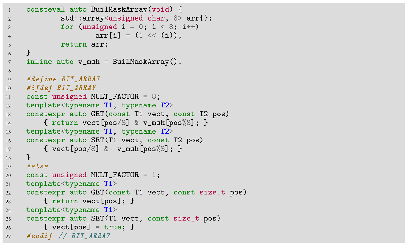
For the first objective, the established solution is to represent the candidates not as a set of values per se, but as a vector of booleans; the value of the candidate is indicated by its position in the vector, while the status (prime or composite) of that candidate is codified through its value. At first the size of the vector element was one interger, as in [5,6], or byte, but very soon the bit representation described in [8] gained more and more traction. The bit compression technique involves bit manipulation using code like the following or similar. Modern compilers will optimize division and modulo with powers of two operands into very fast bitwise operations (division will be replaced with a bitwise right shift, and modulo with a bitwise AND operation) so it is better to leave them as such for clarity; nevertheless, when the compiler is less advanced (like when writing the kernel for GPGPU), it is indicated to write directly in the code the bit operations.
Algorithms 17 00291 i001
Nevertheless, both strategies—bit and byte representations—are currently in use. The bit representation offers clear advantages in terms of memory footprint and especially cache efficiency. However, on lesser CPUs, the additional overhead can sometimes negate the performance gains. Furthermore, when processing the same buffer in parallel, such as with GPGPU, synchronization issues may render the bit representation impractical.
The second objective, minimizing the set of candidates, was also of interest from the start; even the very early algorithms skipped over even values [5] or used the 6 k ± 1 pattern [6]. The 30 k + i pattern (where i { 1 , 7 , 11 , 13 , 17 , 19 , 23 , 29 } ) was also established quite a long time ago; coupled with the bit compression of the buffer, this method is able to represent an interval of 30 in only 1 byte and is the preferred technique for practical sieves today. We have to mention that the first record of this idea dates to as early as 1969 [8].
The problem with such patterns is that they involve complex logic to address the exact position in the vector, often using  if..else  or  switch..case  constructions, which are quite detrimental to performance. A very clever solution for the 6 k ± 1 pattern is to use the fact that the distance between each of two consecutive values alternates the step between 2 and 4; thus, in loops, we can always manage it like this (as introduced in [6]):
Algorithms 17 00291 i002
Yet, this straightforward loop-based approach is not always applicable; most algorithms require the numeric values to be converted into into buffer indexes and back, and here, logico-arithmetic functions like the following were the rule:
Algorithms 17 00291 i003
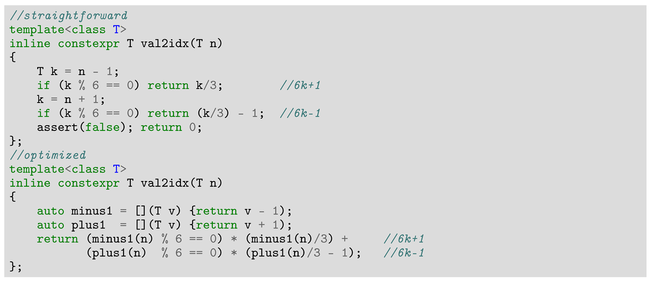
But even these optimized accessors are quite heavy, and for this we devised the following versions for the 6 k ± 1 pattern that are extremely light in comparison:
Algorithms 17 00291 i004
We attempted to apply this approach to the 30 k + i pattern, but achieved only partial success:
Algorithms 17 00291 i005
All the operations involving powers of two are very well optimized by the compiler; there are only two divisions that look difficult, but those are divisions by constant and, again, the optimizing compiler will transform them in very fast shift/mul ops. This arithmetic function is six times faster than the logical variant, but unfortunately we failed to come up with a reasonable inverse one; still, we are certain that somebody can do much better than this.
Our main contribution regarding sieve buffer structure was to introduce, substantiate, and generalize an approach based on residual classes to the sieving buffer and to the sieving process in general. Inspired by the Sieve of Atkin (SoA), where different quadratic forms are employed for different residual classes of 12, the initial idea was to process each of these residual classes separately and in parallel; the next step, to also differentiate the buffer per residue class, was immediate, resulting in four distinct buffers for SoA, corresponding to the four residual classes of interest: 1 (mod 12), 5 (mod 12), 7 (mod 12), and 11 (mod 12). As explained in [23], this approach not only compresses the buffers for even better cache intensity and facilitates the parallelism of the algorithm, but also has an impact on the number of operations itself, as the modulo arithmetic simplifies the operations and helps reduce the set of sieving numbers.
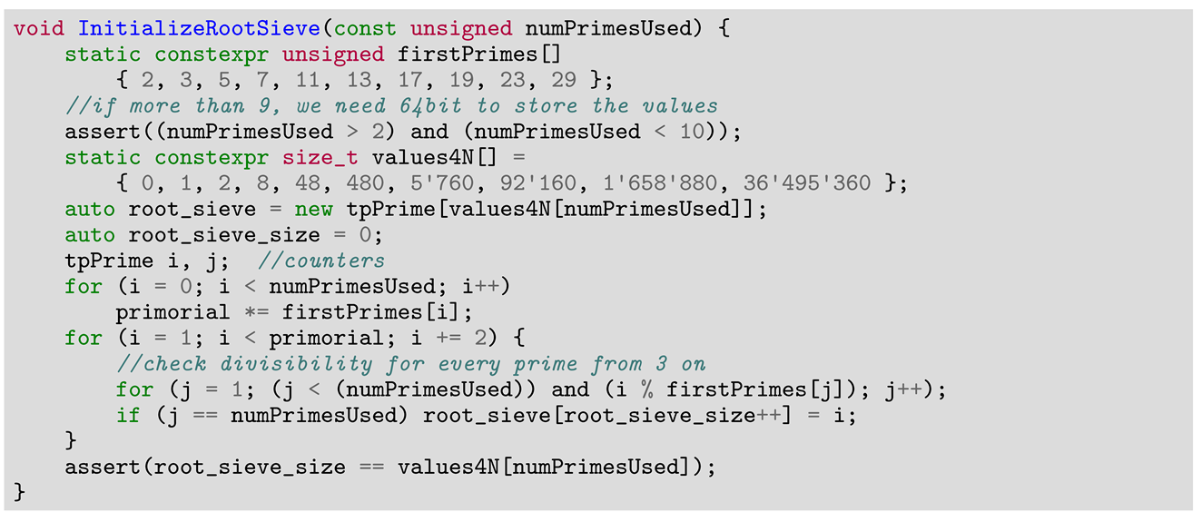
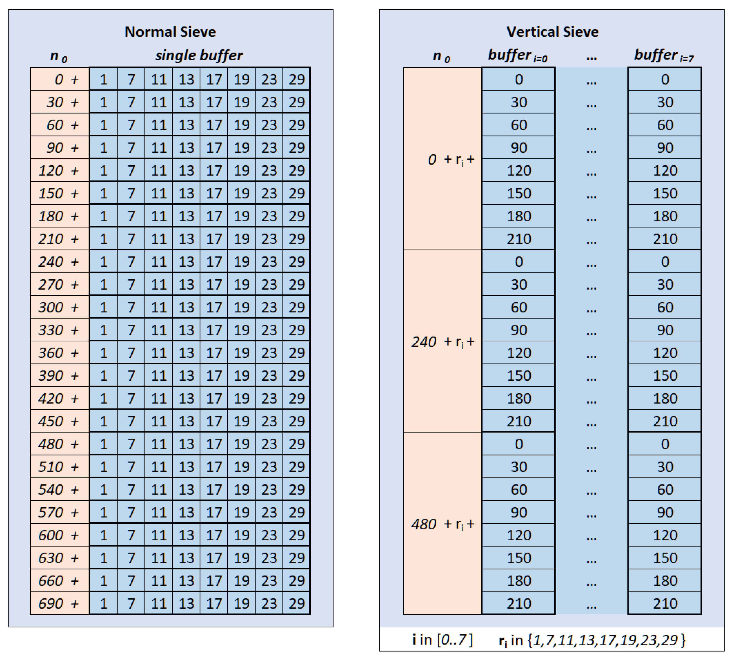
An extension of this idea to the classic wheel of 3 (W3 = { 1 , 7 , 11 , 13 , 17 , 19 , 23 , 29 } ) was introduced in [24] and was generalized in the same paper as the vertical sieve, as illustrated in Figure 1 for W3. The generalized vertical sieve works on distinct buffers, one for each residue class corresponding to the members of a wheel (wheel values). W3 has eight members, and thus eight buffers. W5 has 480, and W7 already has 92,160 members. The next one, W8, does not seem to be practical anymore, with more than 1.5 million members. While the basic sieving operations are somewhat simplified by the modulo arithmetic, when it comes to segmenting the sieve, the initial positioning for each segment is more cumbersome; the same paper [24] gives a generic solution for this problem and provides a very fast implementation up to W7, which, benchmarked against primesieve [25]—the current golden standard in sieving—demonstrates the efficiency of the vertical sieve.

2.2. Sieving

Analyzing all the sieving algorithms known so far, as presented in [22], there are several distinct sieving strategies that emerge:
  • brute-force sieving, using techniques like trial division or other primality testing methods—those should not really be considered sieving techniques.
  • directly sieving a buffer of candidates using a smaller set of primes to sieve out composites—all the sieves based on classic Eratosthenes, including the linear family of sieves, fall in this category.
  • sieving based on mathematical expressions—there are two distinct cases here:
    Sieve of Atkin—directly sieves a buffer of candidates, but using a number of quadratic forms to establish the primality; nevertheless, in the last step of the sieving process, a small set of primes is still required to sift out efficiently the multiples of squares.
    Sieve of Sundaram—indirect sieving: the sieving is carried out using a bilinear form ( 2 i j + i + j ) on a contiguous set and the primes are obtain indirectly from the remainders of that set, after sieving; there are no known methods to reduce the initial contiguous set to be sieved or to reduce the set of factors (the is and js from the 2 i j + i + j form) involved in sieving—given the current knowledge, it seems that this algorithm can only be optimized at the level of the software implementation.
  • iterative sieving: Sieve of Pritchard, a case in itself—the sieving is carried out iteratively, on larger and larger sets of candidates, each set being optimally generated in the previous iteration and sieved using the previous set.
As we can see, all the practical sieves (Atkin and all SoE-based variants) use a smaller set of prime numbers to sieve out composites; the smallest set of primes necessary to sieve primes up to N includes all the primes up to N . We call this set the root primes. And, backtracking, to generate the root primes, we need an even smaller set of primes, which we call seed primes, up to N . For the largest values that are directly manageable by our 64 bit computers ( N = 2 64 ), root primes are limited at 2 32 (a total of 203,280,221 primes) and seed primes at 2 16 = 65,536 ; there is a maximum of 6542 seed primes here, which can be generated extremely fast.
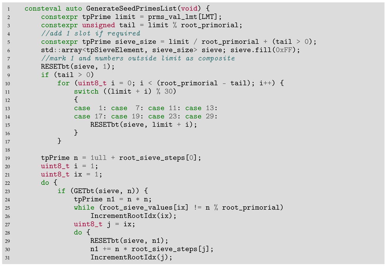
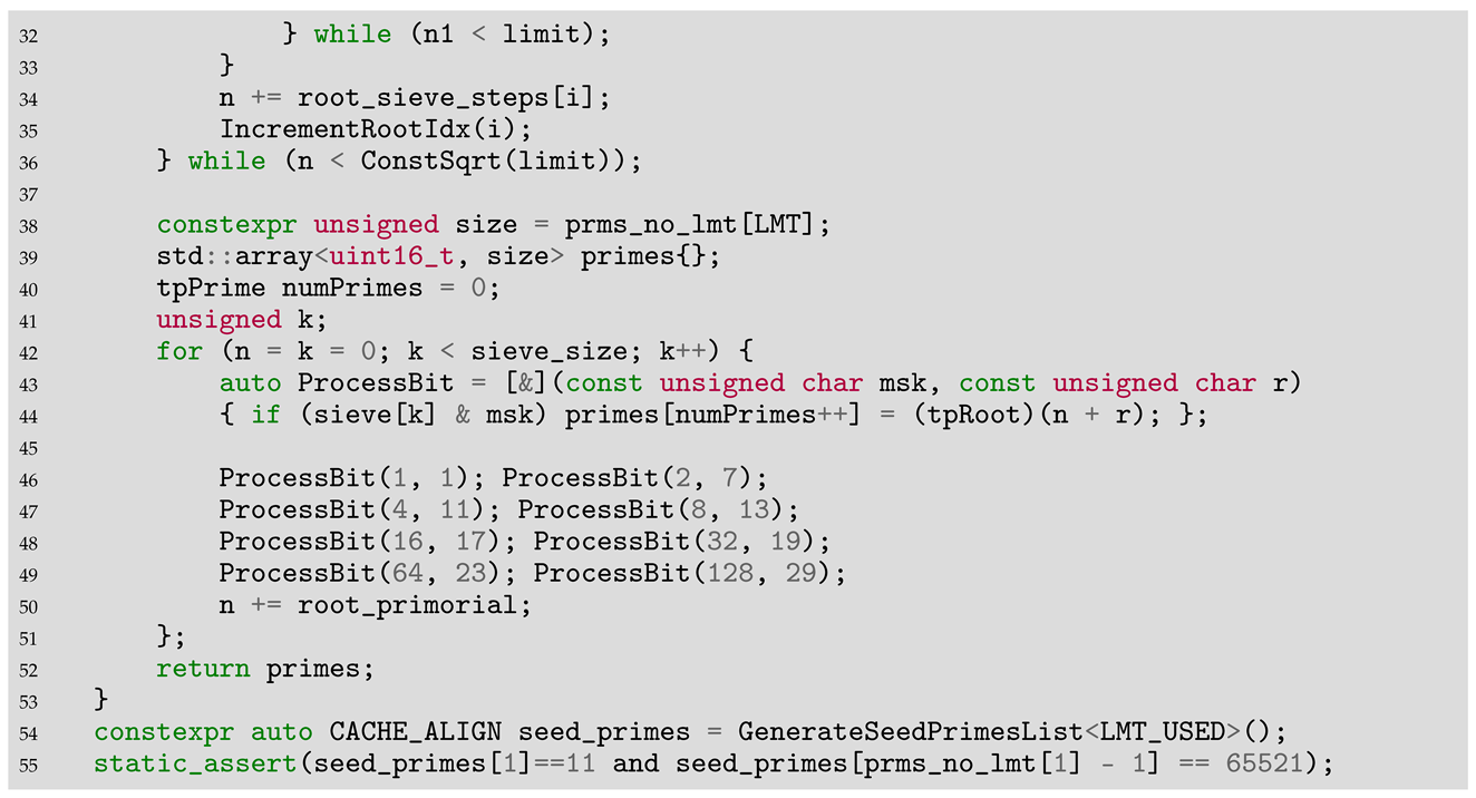
Nevertheless, many practitioners prefer to hard-code them in a vector directly in the source code, which is a little dangerous, as one can inadvertently alter a value without noticing, which will result in strange errors. A safer method is to generate the seed primes at compile time, using code like the following:
Algorithms 17 00291 i006
Algorithms 17 00291 i007
The clear advantage of such methods is to guarantee either correct values or compiler errors.
Another topic is the storage of the root primes. Those more than 203 million root primes required to sieve intervals up to 2 64 , if stored in their native form (4 bytes), would take almost 800 MB of memory, which is quite substantial; on the other hand, as the greatest gap between two consecutive primes lower than 2 32 is 336 (which occurs at 3,842,610,773, the 182,837,804th prime; the next gap is 354, at 4,302,407,359, the 203,615,628th prime (https://t5k.org/notes/gaps.html, accessed on 11 June 2024)): two bytes would suffice for storing only the gap, considering that this list is always parsed in order so performance reconstituting the primes is not an issue. But then, as all prime gaps are even (except between 2 and 3, the only exception there is, as 2 is the only even prime) and 336 / 2 < 256 , we could store the values halved, using only one byte per gap and thus spending only 194 MB for the root primes, which is especially useful when sieving on GPUs (Graphics Processing Units), where global memory can be an issue. The very simple operations involved here—add, sub, shift—practically do not impact the performance, occupying slots that most probably would be otherwise left unused in the parallel pipeline of the processor.
Once we have the sieving buffer and the root primes in place, we can begin the sieving process. However, as any execution profiler will reveal, for any well-optimized implementation, the bottleneck lies not in arithmetic operations but in memory access, specifically memory updates. During the sieving process, the majority of memory updates occur for the smaller prime numbers whose multiples need to be sieved out. For instance, when sieving up to 1000 and skipping over even numbers, the primes 3 and 5 will generate 527 updates, while the prime 7 will generate 136 updates. In contrast, all other root primes will trigger only 248 updates in total. However, the pattern of these updates generated by small primes is repeatable. This exact pattern will repeat identically for each set of 3 × 5 × 7 = 105 values. This period, 105, is the least common multiple (LCM) of the small primes in question, and the period equals the LCM because these numbers, being prime, are all coprime. This repeating pattern is a fundamental property exploited by sieve algorithms, allowing for efficient calculation and elimination of composites. Each time you progress past this interval (in this case, 105), the pattern of multiples that have been marked or eliminated will start over identically. This facilitates the extension of the sieve to larger numbers without rechecking the divisibility by these smaller primes.
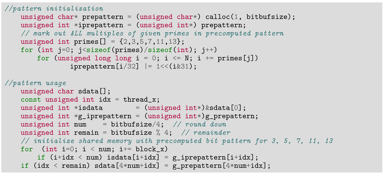
As you add additional primes, such as 11 and 13, the pattern will extend to 15,015 and reach 255,255 with 17. This characteristic is utilized by many fast sieving implementations through an initial phase typically known as pre-sieving. In this preliminary stage, the pattern is generated in advance, usually at the bit level and going up to 13 or 17. Then, during the main sieving process, this pre-generated pattern is used to initialize the sieve buffer at the start of each iteration. This effectively removes all operations related to the small primes that formed the pattern, streamlining the sieving process. Here is such an example of pre-sieving inspired by a basic CUDA implementation from 2009, contributed by Christian Buchner (https://forums.developer.nvidia.com/t/sieve-of-erastothenes/11567/16, accessed on 11 June 2024):
Algorithms 17 00291 i008
Of course, 2, 3, 5 are skipped anyway using static wheels like W2 ( 6 k ± 1 ) or W3 ( 30 k + i ). Larger wheels will skip more small primes, and W7 will exclude by default all small primes up to 17 inclusive, which will eliminate the need to use pre-sieving or will push the pre-sieving limit from 17 to larger primes, as the LCM of those primes does not have to account for the primes avoided by the wheel. Thus, with W7, which was made possible by our generalized vertical sieve, a pattern using 19, 23, and 29 will have a period of 19 × 23 × 29 = 12,673, which is very feasible; even adding 31, we are below 400k, in the same range as the usual pattern 17 of today.

3. Parallel Sieving Strategies

3.1. Generic Considerations

Figure 2 depicts the generic sieving process for a modern, fast sieve. First, the pre-sieving phase initializes the list of root primes and the pre-sieved bit pattern. Then, the sieving continues segment by segment, in parallel. There is much to discuss for each component involved in this process. We have already covered the main data structures (seed and root primes, pre-sieved pattern, sieve buffer). This section will focus on the primary tasks involved in the sieving process.
The simplest tasks might seem to be generating the bit pattern and initializing the sieve buffer with it. However, the initialization is not straightforward, especially when using more complex bit compression schemes, such as the 30 k + i pattern. The approach shown earlier is still viable but somewhat heavier. Ideally, one should superimpose the pre-sieved pattern by copying the bit pattern memory block onto the sieve, over and over, until the end of the sieve buffer. But, with bit compression and such a non-uniform pattern, there are eight pattern variants (each shifted 1 per bit), leading to a performance gain when replacing numerous bitwise operations with relatively few contiguous memory copies.
Nevertheless, this gain comes at the cost of increasing the memory footprint of the bit buffer by eight times. While this increased memory usage might be negligible up to prime 13, it becomes substantial with larger primes. For instance, adding prime 17 increases the memory footprint to 2 GB, and prime 19 to 4 GB. Despite this, the performance gains typically justify the increased memory usage, and it should not pose a problem with a segmented algorithm on modern computers.
The other part of the pre-sieving process, the small sieve, can also be implemented in a variety of ways. Sieving for those 203+ million primes is not immediate. Some implementations handle the small sieve separately from the main sieve, potentially using different algorithms or parallelization strategies. They may even restart the main sieve from scratch, although the sieving is already performed up to 2 32 . Others may use the exact same sieve for both stages, dealing with the added complexity required to differentiate root primes from the rest of the output.
The bulk of the process occurs during the segment sieving phase. This phase is typically executed using a combined parallel–incremental approach; segments are allocated to execution threads and processed in parallel. Within an execution thread, the segment is divided into chunks according to L1 and L2 cache sizes and processed iteratively, sequentially, chunk by chunk. Segmentation is employed for parallelization, while incremental processing is used to maximize cache intensity.
Since sieving is highly sensitive to cache efficiency, maintaining an optimal cache-to-thread ratio is crucial. Usually, implementations employ a 1:1 ratio relative to the available native threads. However, it can be experimentally determined that a slightly higher ratio may be optimal, as modern CPUs employ sophisticated cache management strategies.
After sieving, each thread processes its sieved chunk to generate or count the primes. This is a uniform, linear process and is less dependent on intentional cache strategies because it parses the buffer unidirectionally in read and write operations. Prefetch mechanisms for sequential memory access will almost always keep the relevant data in cache, resulting in minimal latency.
If the goal is solely to count the primes, additional threads can be launched to process smaller pieces of the chunk. This approach can be significantly faster than having the main segment thread perform the task single-threadedly. To reduce overhead, counting threads can be kept idle and then released simultaneously for counting using a simple synchronization mechanism.
If the primes need to be generated in order, a multi-threaded approach introduces some complications, but the overall performance can still be improved with the use of extra threads.
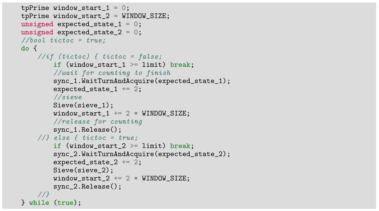
The method described here alternates between sieving and counting. However, these two tasks differ significantly in how they utilize CPU pipelines and their data access patterns. Therefore, overlapping them may lead to better utilization of CPU resources. By concurrently performing sieving and counting, the CPU can be more efficiently exploited, as it can handle the distinct demands of each task in parallel, potentially reducing idle times and improving overall performance. Such a strategy is exemplified in [24], using a so-called tic-toc mechanism which involves two distinct sieving buffers that are processed alternately by the working threads; while one buffer is being sieved, the other buffer is being counted (tic), then the buffers are switched (toc). Here is the gist of the main loop in such an implementation:
Algorithms 17 00291 i009
The counting loop is practically identical, except its states are initialized with 1. Overlapping the two working patterns and fine-tuning the number of sieving and counting threads may result in a better utilization of CPU pipelines.
To conclude the process, the final task is to collect and organize the many lists of primes (one for each segment), which are not necessarily produced in order. This problem is essentially identical to the one encountered within an individual segment if parallel counting is employed. Given that we may need to address the same issue here, it is straightforward to use the same solution in both places.
One effective solution is to have an additional parallel thread that waits for segments/chunks to produce their results and then processes them in the correct order as they become available. This approach ensures that the primes are gathered and ordered efficiently, leveraging parallel processing to maintain performance.
Finally, for testing or benchmarking, there arises the question of how to handle each generated prime. The task must be lightweight enough to avoid skewing the performance metrics, yet substantial enough to ensure the compiler actually computes the prime and passes it to a designated location. Here is our solution of choice for this problem; it works without congestion in a multi-threaded execution, the index does not require any limit check (255 + 1 = 0), and it allows visibility of the last 256 primes generated and facilitates prime validation when single-threaded:
Algorithms 17 00291 i010

3.2. Massive Parallel Sieving

A highly effective strategy for managing the immense computational demands of sieving is to employ a GPGPU paradigm, leveraging the substantial throughput capabilities of GPU devices. To achieve this, it is essential to utilize a framework or SDK that abstracts the complexities and diversity of specific GPUs, providing a generic API. Prominent options include CUDA (perhaps the most widely used framework today, but limited to NVIDIA hardware), Metal (specific to Apple devices), Vulkan (a newer contender in the GPGPU area, though not yet widely adopted), and OpenCL.
OpenCL is a mature platform currently at version 3, supported by major vendors such as NVIDIA, AMD/Xilinx, and Intel, as well as many smaller players. OpenCL also targets devices like FPGAs and various niche hardware from companies like Qualcomm, Samsung, and Texas Instruments. Its practical utility is significant, given that an OpenCL program can run on any OpenCL platform, including most CPUs. Due to its extensive support and versatility, OpenCL is particularly useful. Many professionals are already familiar with CUDA, so this approach will not be used here; instead, GPGPU algorithms will be exemplified using the C++ wrapper (https://www.khronos.org/opencl/assets/CXX_for_OpenCL.html, accessed on May 2024) of OpenCL (https://www.khronos.org/opencl/, accessed on May 2024).
For those familiar with CUDA, we must emphasize that OpenCL and CUDA are quite similar in essence; both are parallel computing platforms designed to harness the computational power of GPUs for general-purpose computing tasks, providing frameworks for parallel computing on GPUs. They allow developers to write programs that execute in parallel on the GPU, taking advantage of the massive parallelism inherent in GPU architectures. Both OpenCL and CUDA use a similar programming model based on kernels (small functions that are executed in parallel across many threads on the GPU) and provide memory models tailored for GPU architectures (different types of memory, e.g., global, local, constant, with specific access patterns optimized for parallel execution). Both platforms organize computation into threads and thread blocks (CUDA) or work-items and work-groups (OpenCL). These units of parallelism are scheduled and executed on the GPU hardware.
The initial tendency when addressing a sieving problem using GPGPU might be to adopt a simple method, where a kernel is launched for each value to be processed. Typically, this is not advisable, because such an approach struggles to handle race conditions effectively: when multiple threads execute simultaneously without proper synchronization, race conditions occur, where the threads attempt to modify the same variable concurrently (in the context of sieving algorithms, if each GPU thread is assigned to mark multiples of a specific prime number, threads may interfere with each other when updating shared data structures like arrays, which can lead to errors or inconsistent results).
Such approach also fails to make use of the GPU’s local data cache: GPUs are most efficient when they can leverage their fast, local memory (like shared memory among threads in a block) instead of relying on global memory, which is slower to access. A simplistic approach where each thread deals independently with marking composites may not effectively utilize this local memory. Algorithms optimized for GPUs often try to maximize data locality to reduce memory access times and increase throughput.
Moreover, launching a separate kernel for each composite to be marked is typically inefficient. It involves considerable overhead in terms of kernel launch and execution management. Efficient GPGPU algorithms usually minimize the number of kernel launches and maximize the work performed per thread, often by allowing each thread to handle multiple data elements or by intelligently grouping related tasks.
To optimally exploit the hardware resources we should implement the sieving algorithm at hand with non-trivial kernels and split the sieving process between the host CPU and device GPU, as in Algorithm 1.
Algorithm 1 Generic CPU-GPU cooperation for sieving
This algorithm splits work between host and device(s), using the GPU(s) mainly for sieving itself.
  • Initialization
    •  Initialize the GPU device, create a context, allocate memory buffers, and compile/load the kernel code onto the GPU.
    •  Set up any necessary data structures and parameters for the sieve algorithm.
    •  Presieve both host- and device-side tasks. Splitting presieve tasks between the CPU and GPU is not trivial: in the early days, transferring data from the host to the device was slow, so it was often faster to generate, for example, root primes directly on the device; new hardware minimizes such issues, so it is best to conduct some benchmarking before deciding where to perform each task.
  • Launching Parallel Threads
    •  The main thread will coordinate the sieving process and handle communication between the CPU and GPU. This thread will manage the overall control flow of the algorithm and coordinate the execution of kernels on the GPU.
    •  Start a parallel thread or process on the host for generating and counting the primes. This thread will work on buffers sieved by the kernel; the thread is initially idle, waiting for the first buffer to process the primes.
  • Loop Kernel Executions
    •  Divide the range of numbers into segments or chunks, each corresponding to a separate interval to sieve for prime numbers.
    •  Iterate over each segment and perform the following steps:
    a. Launching the Kernel:
       - Prepare any necessary parameters or buffers to the kernel.
       - Launch the GPU kernel responsible for sieving prime numbers within the current segment.
    b. Waiting for the Kernel to complete the sieving:
       - Wait for the GPU kernel to complete its execution.
    c. Downloading Sieved Buffer:
       - Wait for the previous counting step (if any) to finish.
       - Transfer the results (sieved buffer) from the GPU back to the CPU.
       - This buffer contains information about which numbers in the current segment are primes.
       - Release the semaphore or whatever sync mechanism in place, in order to signal the parallel counting thread that it can start counting.
    d. Generating Primes (this step is executed in parallel with all others):
       - On the parallel CPU thread(s), wait to receive a new sieved buffer.
       - Process the sieved buffer to identify and generate the prime numbers within the current segment.
       - This step involves parsing the buffer and extracting the prime numbers based on the sieve results.
       - At the end of counting, release the semaphore or whatever sync mechanism to signal the main thread that it can download the new buffer from the GPU.
       - Go back to waiting for the new buffer or exit if finished.
    e. Repeating the Process:
       - Repeat steps a–c and d for each remaining segment until the entire interval is exhausted.
  • Completion and Cleanup
    • Once all segments have been processed and the prime numbers have been generated, finalize any necessary cleanup tasks.
    • Release GPU resources, free memory buffers, and perform any other necessary cleanup operations.
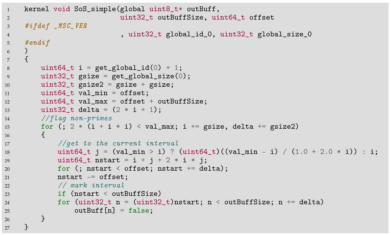
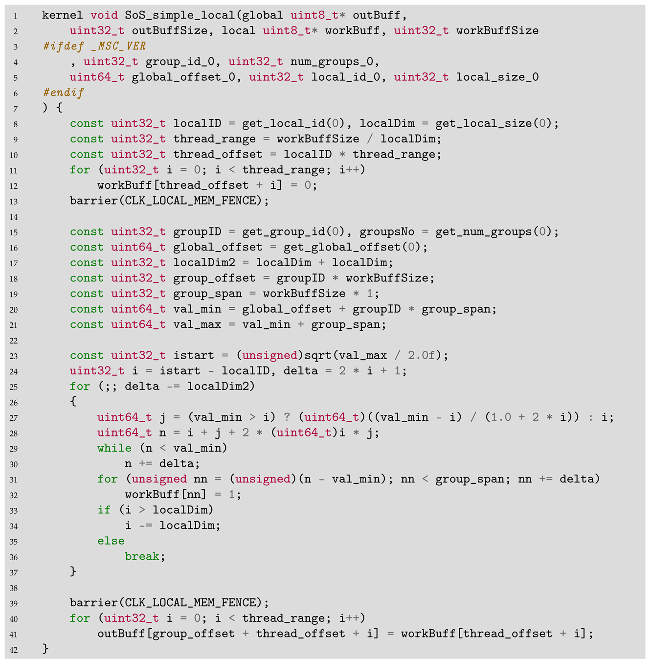
To exemplify a non-trivial kernel, in Algorithm 2, we have a straightforward kernel for a basic OpenCL implementation of the Sieve of Sundaram on a GPU.
Algorithm 2 Sieve of Sundaram—basic kernel
  • Basic additive version, using global memory
Algorithms 17 00291 i011
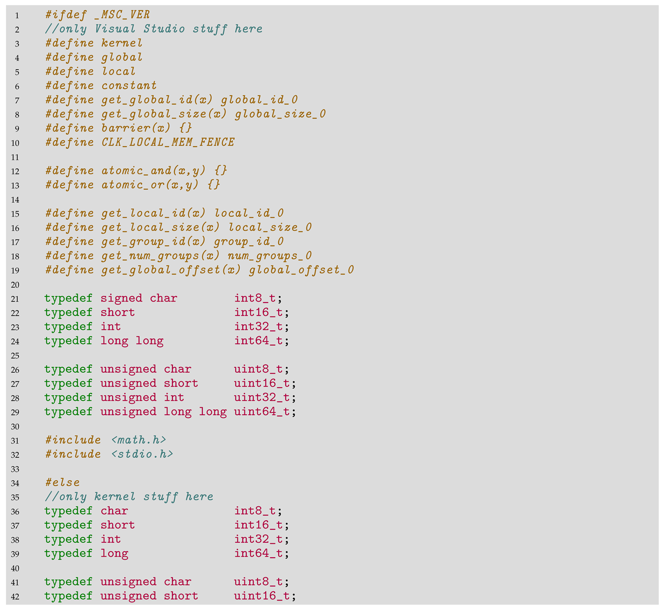
This basic implementation still uses only global memory, but what is particularly interesting is that, inserting before the kernel code some header code like the following:
Algorithms 17 00291 i012
Algorithms 17 00291 i013
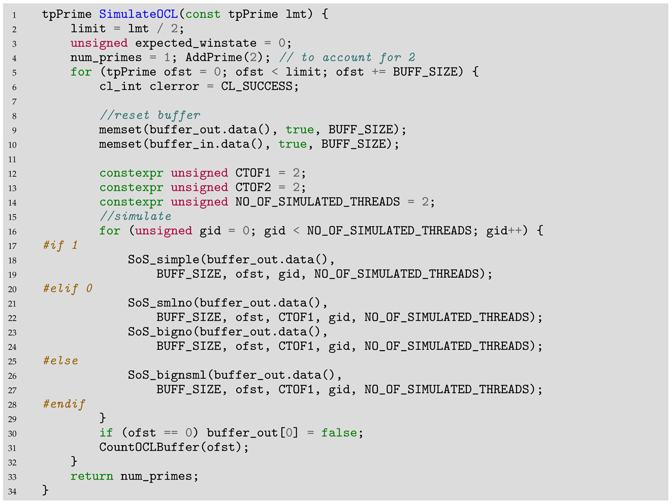
We can also compile and use this kernel on the normal CPU, thus helping with the development process, as compile errors are signalled immediately and most of the logical errors can be debugged using the IDE debugger, which is much easier; of course, more subtle bugs that are specific to a GPU environment will still have to be investigated natively, but in any case, the development process may accelerate significantly. Here is an example for such simulation code using the kernel above as such, but also prepared to use other experimental kernels:
Algorithms 17 00291 i014
The problem with such non-trivial but basic implementations of sieving algorithms is that the internal mechanics of sieving are not linear. Practically all sieves are executed in a nested loop technique; the outer loop iterates a primary parameter, while the inner will iterate a second parameter and the number of iterations varies significantly, usually non-linearly. Yet, while the kernel code exemplified above tries to obey the basic rules of GPU programming—avoid complex operations and 64-bit data whenever possible, and do not count too much on the optimizer—the resulting performance is horrendous; although we exploit thousands of native GPU threads, the performance may very well be worse than a similar basic one-threaded incremental CPU implementation.
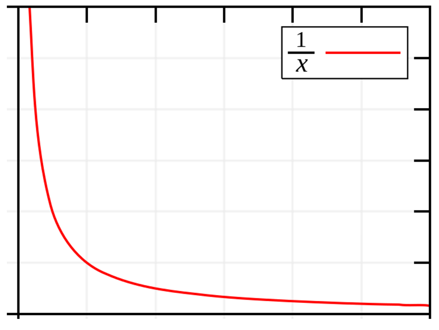
There are some generic explanations involving the lower frequency of the GPU cores, the overall cache efficiency of a CPU, and generally speaking, the huge differences in performance when comparing one-to-one a CPU thread to a GPU one, but the fundamental explanation comes from the fact that those thousands of GPU “threads” are not really independent threads; they correspond with the work-items in OpenCL and are grouped in wavefronts (or warps for CUDA), each consisting of 32 or 64 threads that run in sync. Each thread in the wave will not end until the last thread in the wave has finished all the work, thus keeping the whole CU (compute unit) occupied. Because we are using a stripping approach for domain segmentation, the thread lengths vary significantly within a warp, so the result is that, although the vast majority of threads have finished, a very small number of threads keep everything stalled, and those are the work-items that include is with very small values. While for i above 100, there are only several hundred iterations in the inner loop, for values bellow 10, there are many thousands, something qualitatively similar to function f ( x ) = 1 / x , as in Figure 3. (This particular function— 1 / x —is chosen simply because it is the most well known among those with a similar profile, only to provide an idea of the curve’s profile. The actual function is more complex, but qualitatively, the profile is similar).
Although most of the work is completed in the first hundred milliseconds, a small number of threads will keep working to process all the js for those small is; thus, because the GPU thread is significantly weaker than a CPU thread, we obtain lower performance overall.
The real art in devising a parallel algorithm is to find a segmentation method for the problem domain that is able to evenly distribute the computation effort between segments; basically the goal is to flatten the curve, in order to achieve the best possible occupancy of the GPU. One solution here is to create two different kernels: one very similar to the simple one used above, which works quite well for big values of i, and another one for very small is. The second kernel will transpose the problem, iterating on j in the outer loop, thus surfacing the depth of the inner loop and flattening the curve like in Figure 4. Such a dual big–small-transposed approach will have significantly better results.
Most of the time, a better solution is to use an approach similar to the one for the corresponding incremental/segmented sieve and exploit the local data cache of the GPU CU; mapping each CU to a segment and targeting the local data cache size for the segment buffer size, the curve will be relatively leveled naturally. The overhead for positioning in each segment is mitigated by the fast access of the cache, resulting normally in even better timings. The gist of such a segmented kernel that exploits local a CU cache is exemplified for Sundaram in Algorithm 3.
Algorithm 3 Sieve of Sundaram—segmented kernel
  • Barriers are used to guard local buffer initialization and upload.
  • Optimizing the positioning component (determining the initial i and j values for each segment) was very important.
  • The outer loop is descending for simplified logic.
Algorithms 17 00291 i015
Once we have a decent kernel, the last step in optimizing the sieve is to parallelize the final phase of the sieving process, the actual counting/generation of primes, so that the counting is not longer that the sieving, which should not be difficult; final timings of such an implementation will be driven exclusively by the duration of sieving itself, as executed on the GPU, plus the transfer of data buffers between host and device, which is not negligible. Sometimes, it may be faster to generate initial data directly on the GPU and avoid any data transfer from the host to the device, although modern technologies like PCIe 4/5 and Base Address Register (BAR) Resizing (or Resizable BAR) have improved this issue a lot.
The performance may be further improved by flattening the curve inside each segment using the cutoff–transpose technique, as described above, or avoiding unnecessary loops because, for larger is, only a small number of js will actually impact a certain segment, and a bucket-like algorithm [26] may benefit the implementation.
But perhaps the hardest problem is to avoid collisions between local threads, especially when using on the GPU buffer a 1bit approach for data compression, as we use on the normal CPU; on the GPU, this is particularly difficult, as one has to be sure that in the same workgroup cycle there are not two work items (local threads) that will try to update the same byte, as this will result in memory races that will keep only the last data value and lose the others.
When working with uncompressed buffers (1 byte per value), this issue is not important anymore for Eratosthenes and Sundaram families of sieves, because here, if the values are updated, they are always updated in the same direction: changing from 0/false to 1/true (or vice versa); memory races are not an issue here, as the final result will be correct irrespective of which thread managed to make the update.
For the Atkin algorithm, the outcome is contingent on the starting value, and concurrent operations by two or more threads can lead to incorrect results. For instance, in Atkin, if the initial value is 0 and two threads modify it one after the other, the first thread will read 0 and change it to 1, while the second thread will read 1 and switch it back to 0. However, if both threads operate at the same time, each will read the initial value of 0 and both will write back 1, resulting in an erroneous final outcome. And this problem is valid for all sieve families when dealing with bit compression.
For non-segmented variants the problem is relatively easier to solve, for example, using larger strides (as in Buchner’s example mentioned earlier), thus ensuring that each thread will work on a separate byte. The solutions for this problem are not at all trivial. One illustration of such an efficient approach is given in CUDASieve, a GPU-accelerated C++/CUDA C implementation of the segmented sieve of Eratosthenes [27]; unfortunately, we could not find other detailed examples of such mechanisms.
4. Hard-Core Optimization Techniques

4.1. Advanced Code Optimizations

For each sieve implementation, there are numerous specific make-or-break points where small alterations may dramatically alter the performance. Those are usually in the inner loop; it does not make sense to agonize over some optimization in the outer loop, such as lamenting over a complex sqrt instruction used there:
Algorithms 17 00291 i016
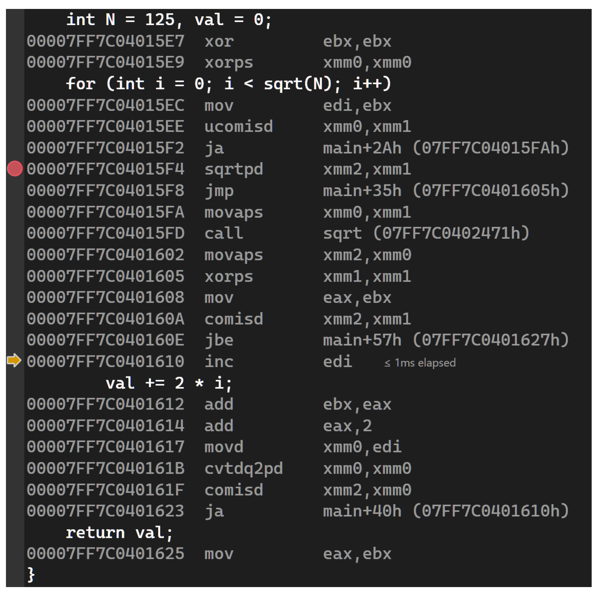
First of all, it is very probable that the compiler will sense that the value of N is not passed by reference anywhere, so it is constant in that block, and therefore, it can be optimized; look at the disassembly code in Figure 5. The line with sqrtpd (red debug point) is reached only once and the square root is stored in xmm2; the end test (ja at 00007FF7C0401623) will jump back at 00007FF7C0401610 (yellow cursor) and loop down without re-evaluating xmm2. Secondly, those instructions are effectively executed millions of times less frequently than those in the inner loop.
One typical example of code that requires careful attention, and which gives us an opportunity for a philosophical aside, is cycling through the indexes in a static wheel, as commonly seen in the case of W3, where the eight values in the wheel may be iterated over many billions of times in a single sieving session:
Algorithms 17 00291 i017
The longer logical variant is exactly as efficient as the shorter one; condensed, prolix code is not necessarily faster. And, most important, the logical variant is not always slower than the arithmetic one, just because it includes a decision that can fool the CPU’s prediction unit and may result in the pipeline being flushed. In fact, in our case, the hardware may be fooled only once every eight instances, which means it will avoid those relatively complex operations seven out of eight times, thus being overall about twice as fast; arithmetic versions are faster only when used against a quasi-random pattern. Do not start optimizing without first profiling and benchmarking the code; after the “optimization”, re-profile the code. Sometimes, the “optimization” will result in a net loss of performance.
One of the heaviest operations for the processor is integer division, especially at 64 bits, as integer division must yield an exact quotient if possible (without any fractional part), which can make the division algorithm more complex (unlike floating-point division, where some degree of error is acceptable due to the nature of floating-point arithmetic, integer division in most programming contexts must provide an exact result if the division is evenly matched: this makes the division process more intricate, especially for large numbers; moreover, floating-point numbers are represented in a format that allows for a trade-off between range and precision, typically using the IEEE 754 standard: this format inherently supports approximations, which can simplify the hardware design for division; the processors are often optimized for high throughput of floating-point operations, particularly in scientific computing and graphics applications—modern CPUs usually have dedicated hardware for floating-point operations, including division, which can execute these instructions very efficiently). Libraries like libdivide (https://github.com/ridiculousfish/libdivide, accessed on 11 June 2024) can obtain a speedup of up to 10× for 64-bit integer division and a speedup of up to to 5× for 32-bit integer division, especially with older CPUs.
Another extreme optimization employed by many sieves in the counting phase is the usage of advanced population counting (counting the number of 1 bits in a vector, akin to counting the number of ones in a binary stream) techniques that speed up as much as possible these operations using specialized CPU instructions, including SIMD instructions; an example of such a library is libpopcnt (https://github.com/kimwalisch/libpopcnt, accessed on 11 June 2024), created by Walisch himself based on [28]. We insist that this approach may give the wrong idea regarding the performance of a sieve, and this performance should be assessed only when we are sure that the primes are really generated and in order; nonetheless, during debug and testing of the sieving phase or when the objective is strictly counting primes, these helpers will boost performance significantly.
For many other very advanced optimization techniques, one should study, perhaps in this order, the source code accompanying the following articles:
  • Bernstein’s implementation of Sieve of Atkin [29]—besides SoA, it includes a relatively advanced cache-intensive incremental SoE generator, demonstrating some advanced techniques.
  • Oliveira original Bucket Sieve implementations [26]—besides the bucket sieve itself, they include some advanced techniques like pattern based pre-sieving with small numbers.
  • Achim Flammenkamp’s prime_sieve [30], the fastest sieve at one point—a lot of techniques that later became widely utilized by many.
  • Original Walisch’s implementation [31]—precursor of primesieve.
  • primesieve [25]—the current gold standard of modern fast sieves, containing most of the advanced techniques.

4.2. SIMD

In traditional programming, operations are typically carried out sequentially. Each instruction is executed one after the other, and each instruction operates on a single data element at a time. This is also known as SISD (Single Instruction, Single Data) execution.
SIMD (Single Instruction, Multiple Data) programming, on the other hand, leverages parallelism by performing the same operation on multiple pieces of data simultaneously. This is achieved by using special hardware capabilities available in modern processors, such as vector registers and SIMD instructions, which can process multiple data points in parallel, resulting in increased performance for tasks that involve repetitive operations on large datasets, as is the case for prime sieves. SIMD is able to process eight data points at once, starting with 8-bit integer data points for MMX (introduced with Pentium) and going up to 64-bit integers for AVX-512 in modern ×86 architectures (modern processors implement various SIMD approaches, using multiple very large registers to compute a certain operation in parallel on several values: Intel started with MMX (64-bit registers), then SSE (128 b), followed with AVX2, which has 256 b registers, thus allowing for 8 × 32 b integers or floats to be operated on in parallel, with a theoretical improvement limit of up to 8×; more recent hardware implements AXV512, where you can work on 16 × 32 b values at ones, using 512 b registers; limiting the code at AVX2 will result in larger compatibility, as AVX2 has been implemented in most CPUs since 2012, with the exception of some Pentium and Celerons; AMD has also largely implemented AVX2, and even AVX512 on many of the last models.). Here is a very simple illustration of SIMD code:
Algorithms 17 00291 i018
Algorithms 17 00291 i019
Still, if you benchmark this code against a standard SISD implementation using the same logic with an optimizing C++ compiler on a modern CPU, you will obtain very similar performance; the use case has to be more complex to obtain a performance boost.
Let us consider the case of generating the static wheel using brute force:
Algorithms 17 00291 i020
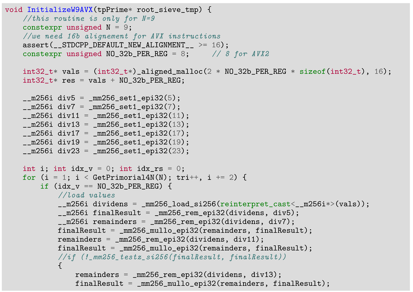
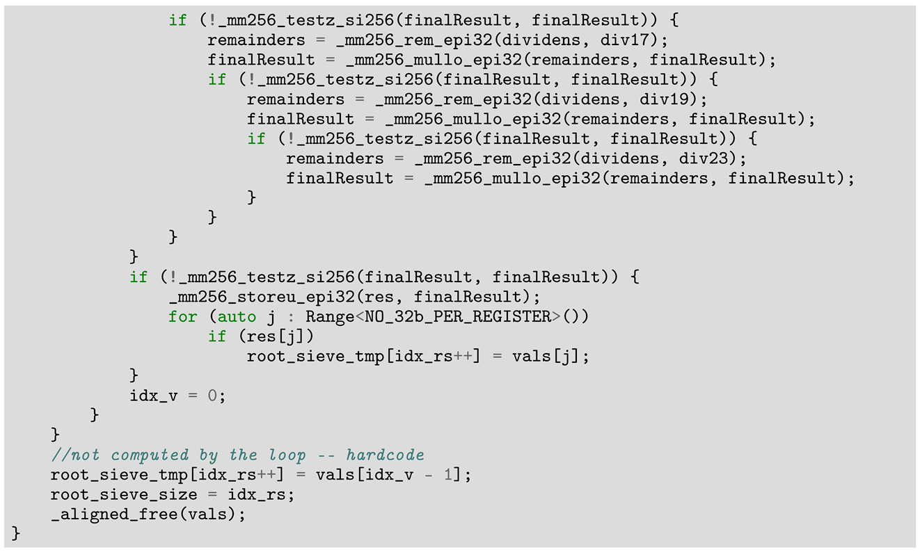
The time consumed by this task is practically 0 for N < 8 ; even for 8, generating 1.6 million values, it is around 30 ms, nothing to optimize for a job running only once per sieve. But the duration changes dramatically for N = 9 , obtaining over 1 s—1150 ms in our benchmark. Here is a similar implementation using AVX2:
Algorithms 17 00291 i021
Algorithms 17 00291 i022
Deep in the inner loop, there are some _mm256_testz_si256 tests to check if it makes sense to go on, as a remainder operation is practically a division, one of the costliest instructions. Thus, testing if we did not already exclude all values, it makes sense, because this is a very light operation, but only if the probability to have values is low. After the first step, it is clear that we will have one or a maximum of two values divisible by 5 from eight consecutive values (eight correspond to 3 × 8 where, multiples of 2 and 3 were culled, but also, 2/3 of multiples of 5 are culled by the loop, so the ratio is preserved). The process is similar for the next step, with 7. For 11, we will have two or three values for each of the three sets of eight, so again it was intuitive that the test there should not be useful. At 13, it is debatable; the benchmarks were not conclusive, so we left the test in. From 17 onward, it is clearer that the test will save precious time, as proved also by the benchmarks. This code will cut down the time for W9 from 1150 ms to 820 ms (measured on an i9-9900KF CPU): apx.25% net gain (if the procedure would be more compute-intensive, we could obtain very impressive results; here, we have quite an important memory access pressure, so the data access pattern will limit the performance gain). Of course, there are better ways to compute the wheel, but using SIMD may have similar effects to the final results.
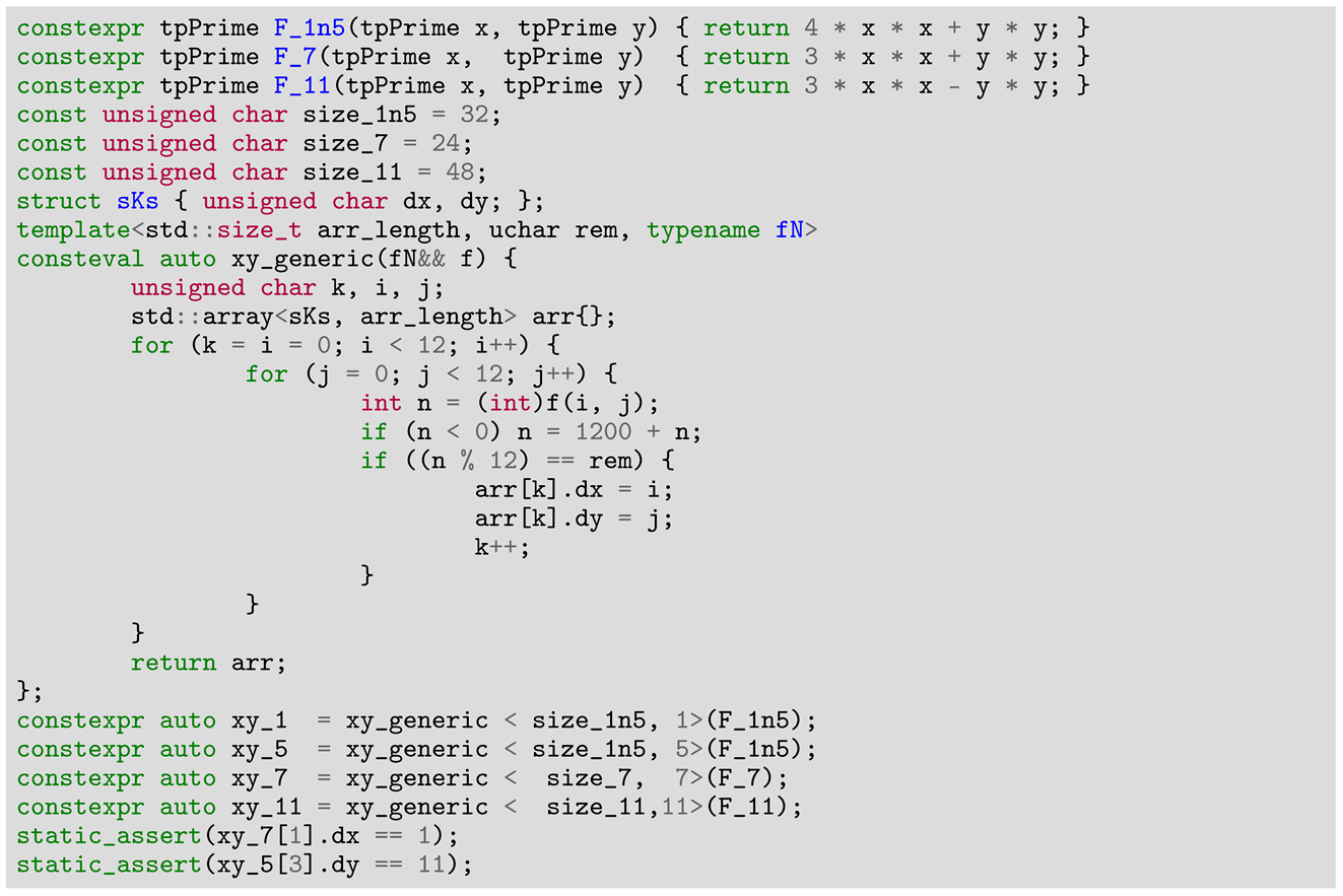
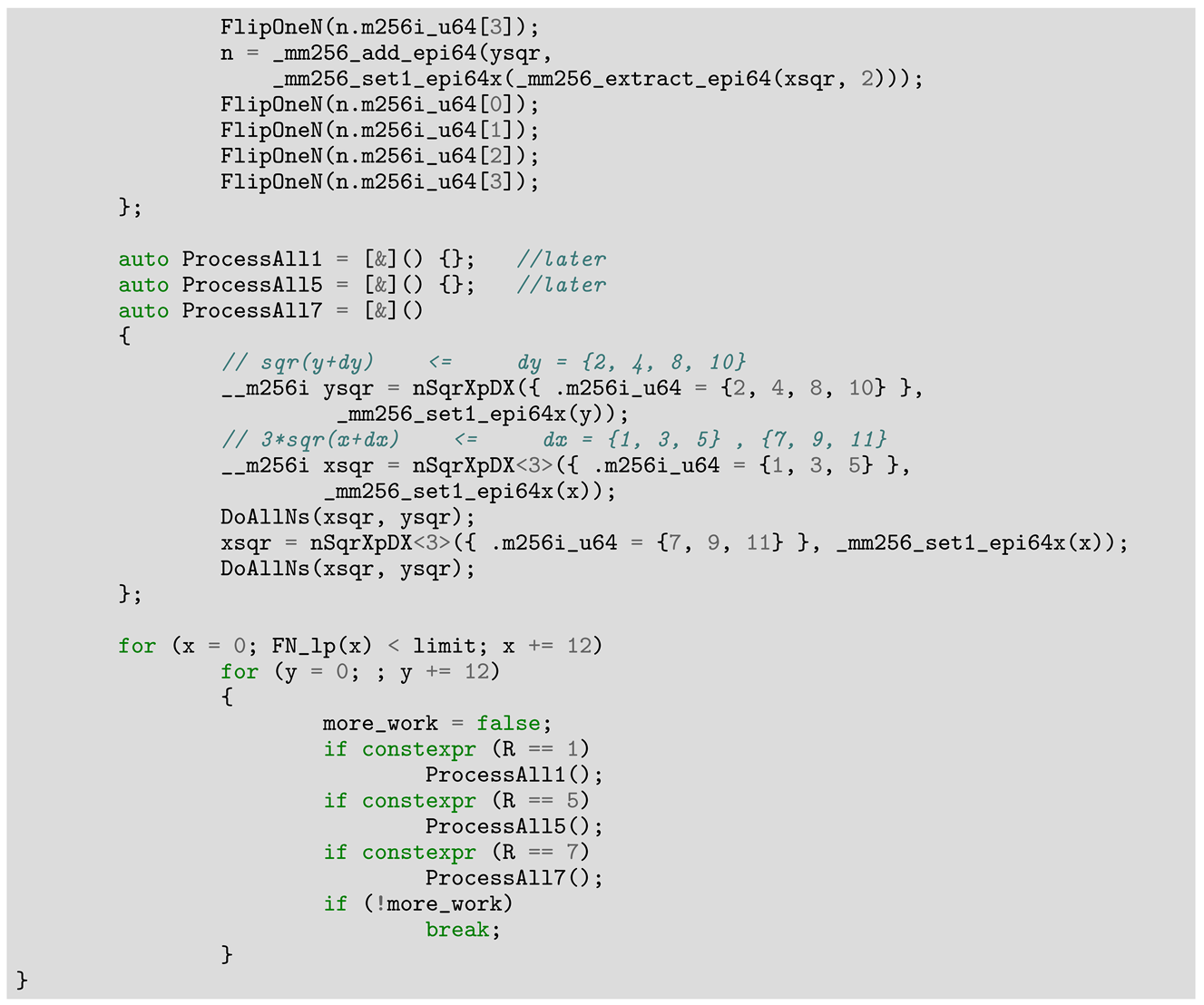
An even better demonstration of the power of SIMD when applied to sieving can be produced with the tuples version of Atkin, as explained in [23]. In that paper, we have identified the full set of tuples that give all the eligible values to be checked by the quadratic forms involved in the Sieve of Atkin, shown in Figure 6. As demonstrated in the article, any quadratic form a x 2 + b y 2 can be expanded like this:
a x 2 + b y 2 = a ( 12 k + i ) 2 + b ( 12 p + j ) 2 = 12 r + a i 2 + b j 2
The remainder of a quadratic form like that is equal to the quadratic form of the remainders, so we can predict the remainder from the factors. If a i 2 + b j 2 = v , then for any k and p, the remainder of a ( 12 k + i ) 2 + b ( 12 p + j ) 2 with d will be v, and vice versa. So, all we have to do to obtain the exact candidates that have the required remainders is to use only those combinations of i and j that generate that remainder.
These tuples can be statically generated with code similar to this:
Algorithms 17 00291 i023
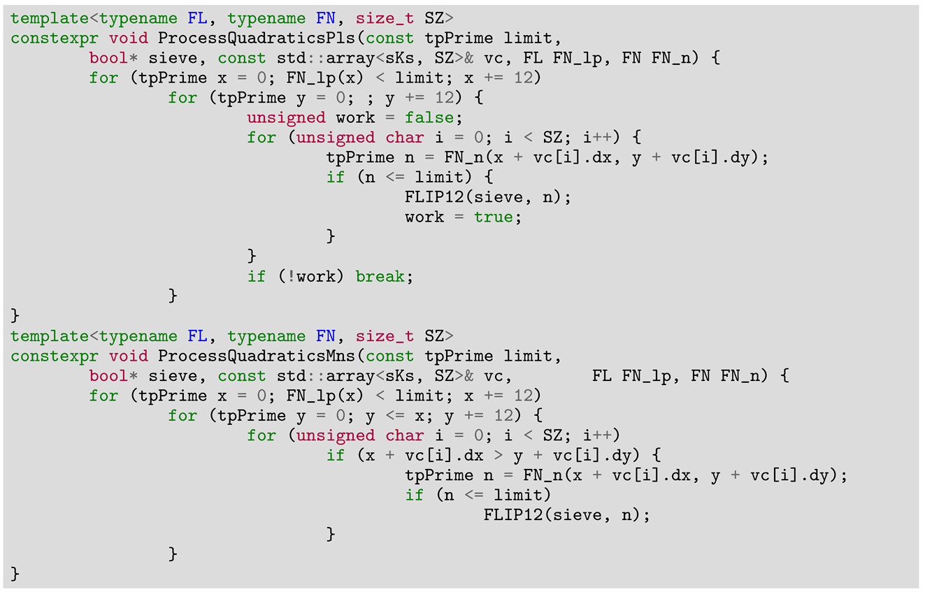
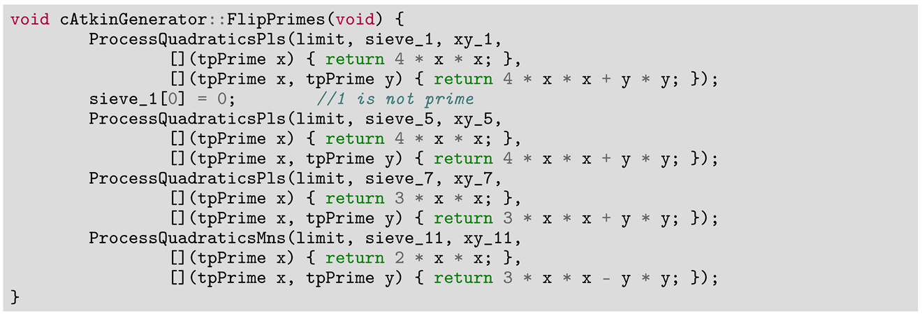
The sieving part of SoA with tuples may look like the following (ignoring the square elimination and counting phases):
Algorithms 17 00291 i024
Algorithms 17 00291 i025
A code like this will sieve up to 1 billion in apx.3600 ms (measured on the same i9-9900KF CPU.).
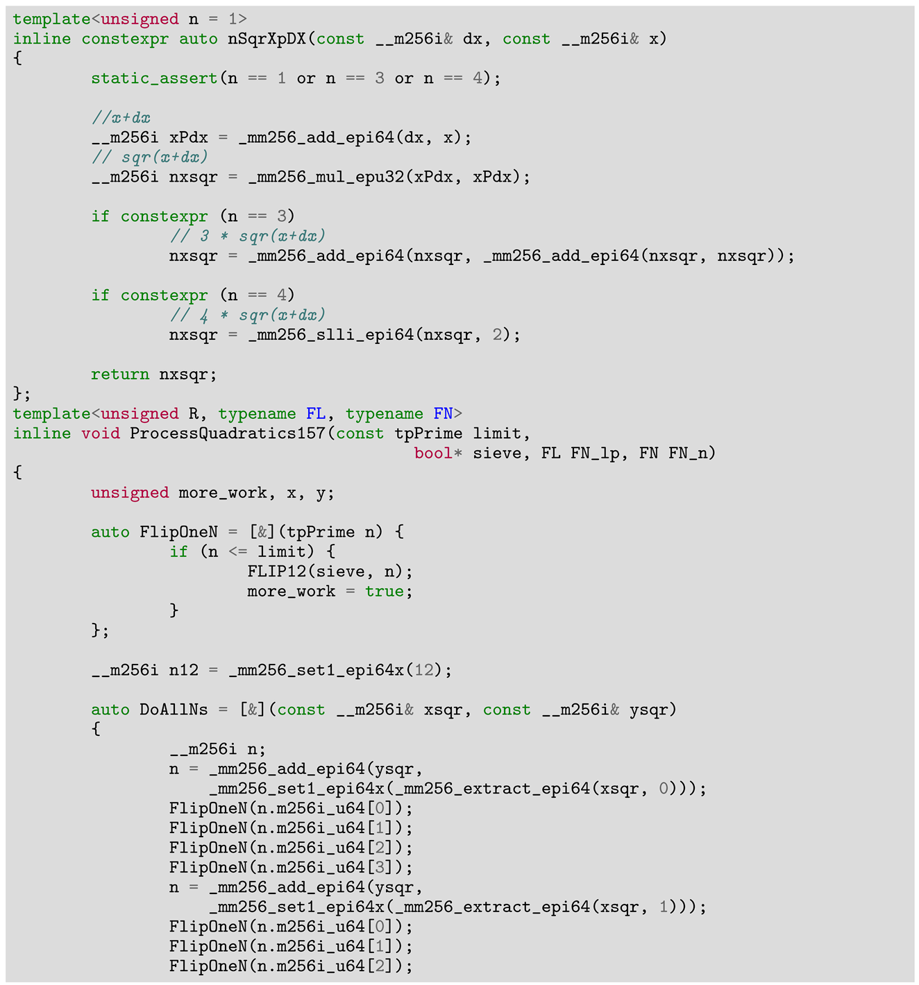
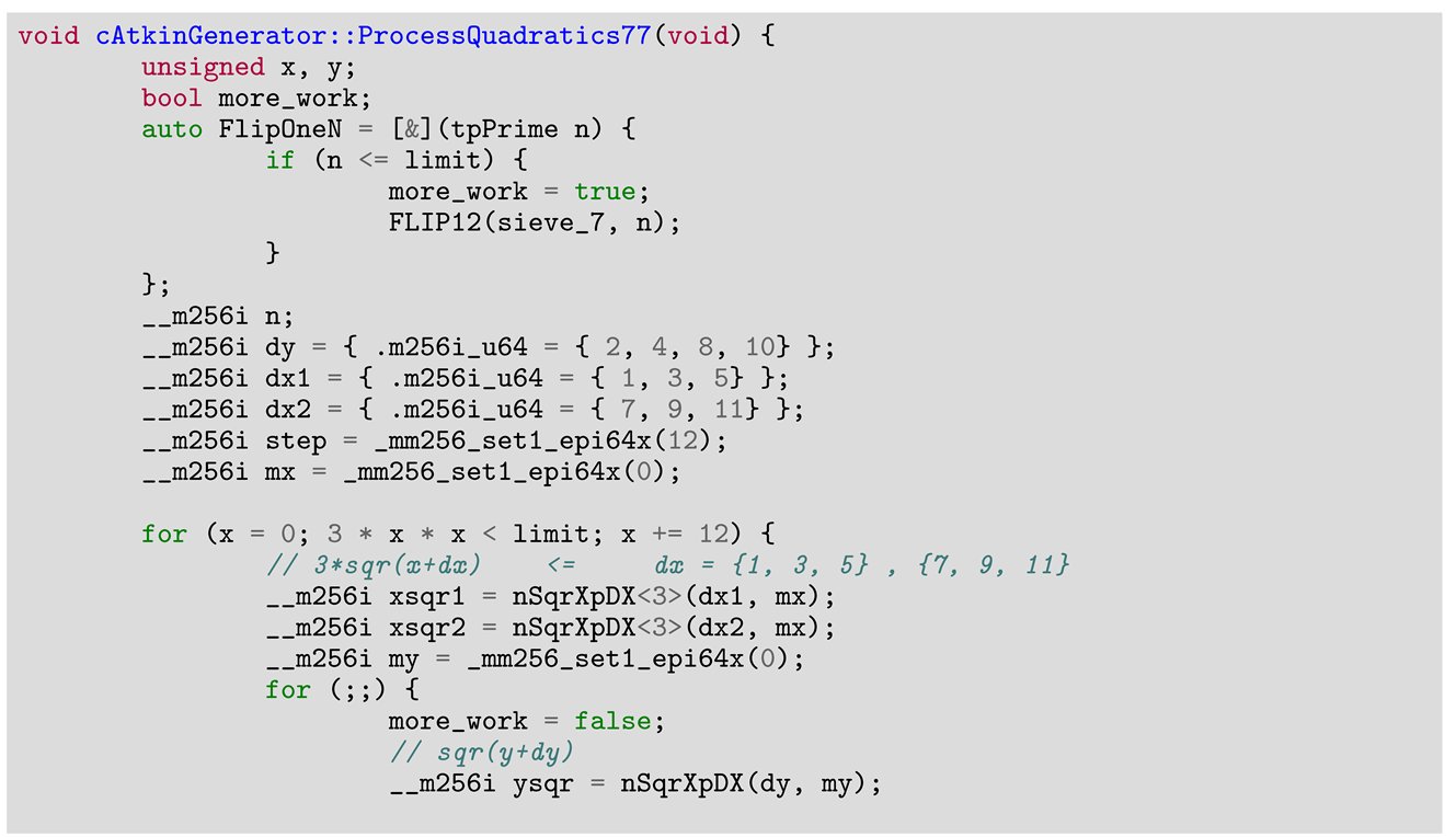
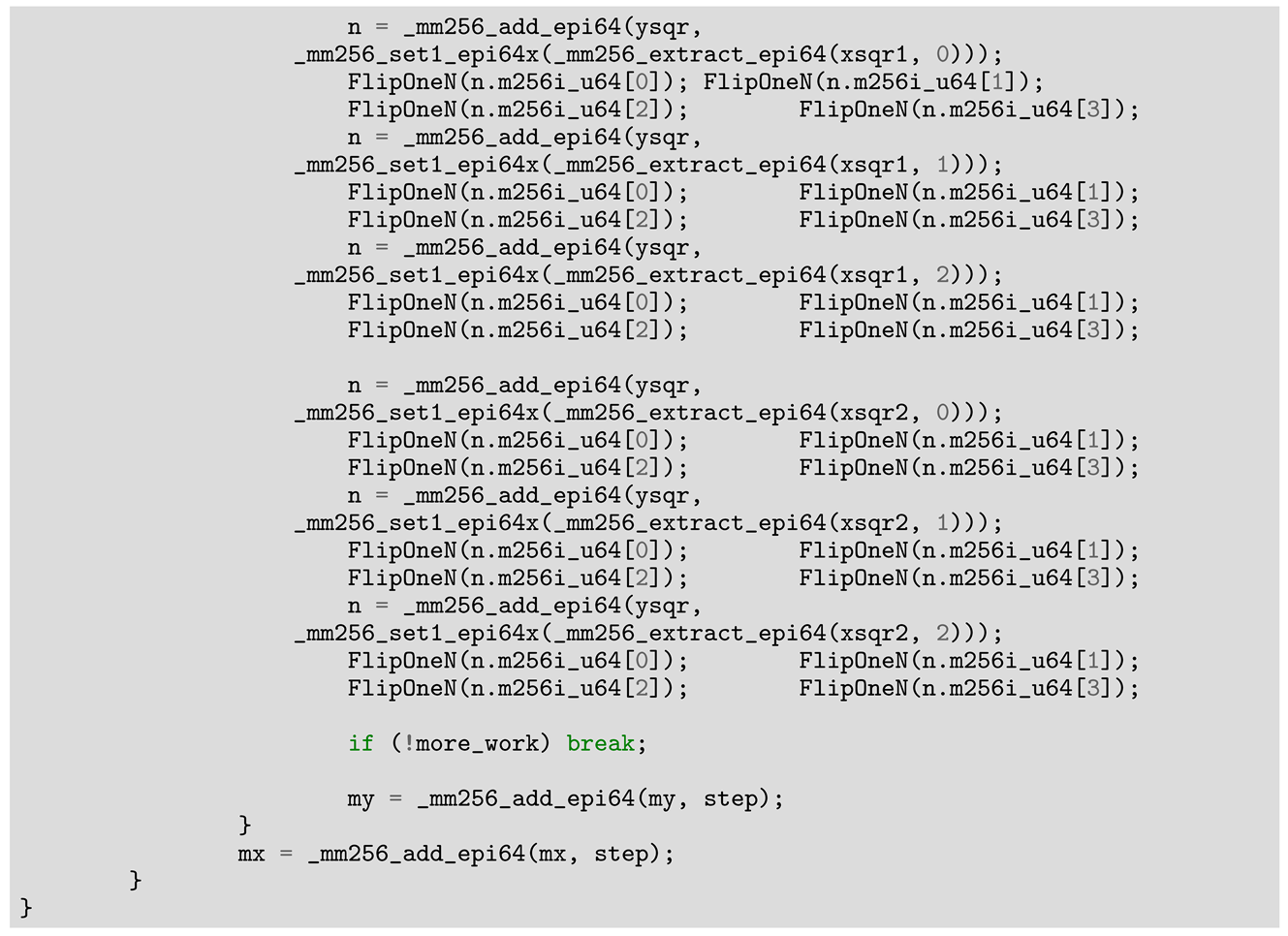
Given the pregnant symmetry and coherence seen in Figure 6, the values of the tuples seem to follow strict patterns; they are not only repetitive, but also mainly grouped in sets of four. {1, 5, 7, 11} and {2, 4, 8, 10} keep repeating, so we should take advantage by processing more than one value at a time. AVX2 works with exactly four 64-bit values at a time, so it is a perfect match for these patterns. Of course, we are tempted to try and preserve code flexibility with templates and lambdas, by coding something like the following (for 7):
Algorithms 17 00291 i026
Algorithms 17 00291 i027
But this approach worsens the performance from 3600 ms to 3900 ms, using SIMD only for 7. Looking at the generated assembler, we see that a lot of data move between memory, ALU (the arithmetic and logic part of the CPU, where normal registers and operations are concentrated), and the SIMD registers, which are somewhat separate in the CPU. In addition, one of the lambdas was not inlined by the compiler; it was left as a function, generating a lot of movement on the stack. Moreover, it turns out that DIV is not implemented natively for integers in AVX2 and that intrinsic was actually generating another heavy call to a library. In conclusion, we need to be less ambitious regarding the flexibility and write a dedicated method:
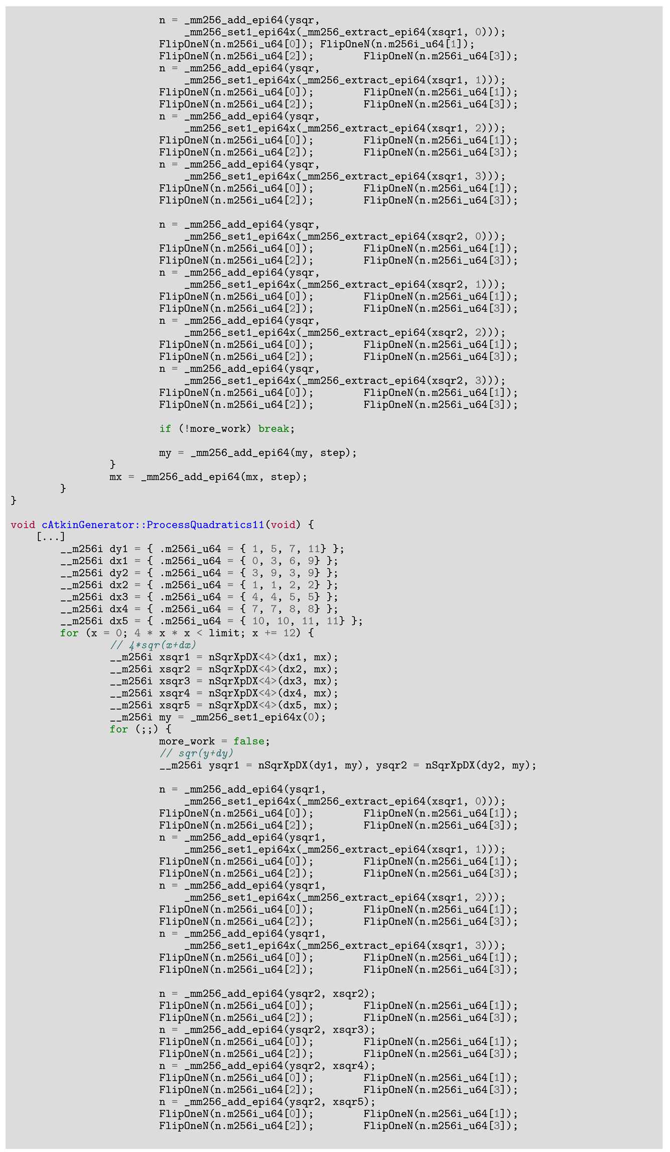
Algorithms 17 00291 i028
Algorithms 17 00291 i029
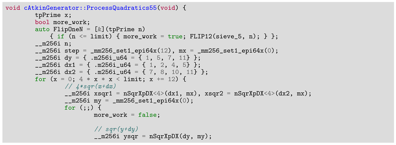
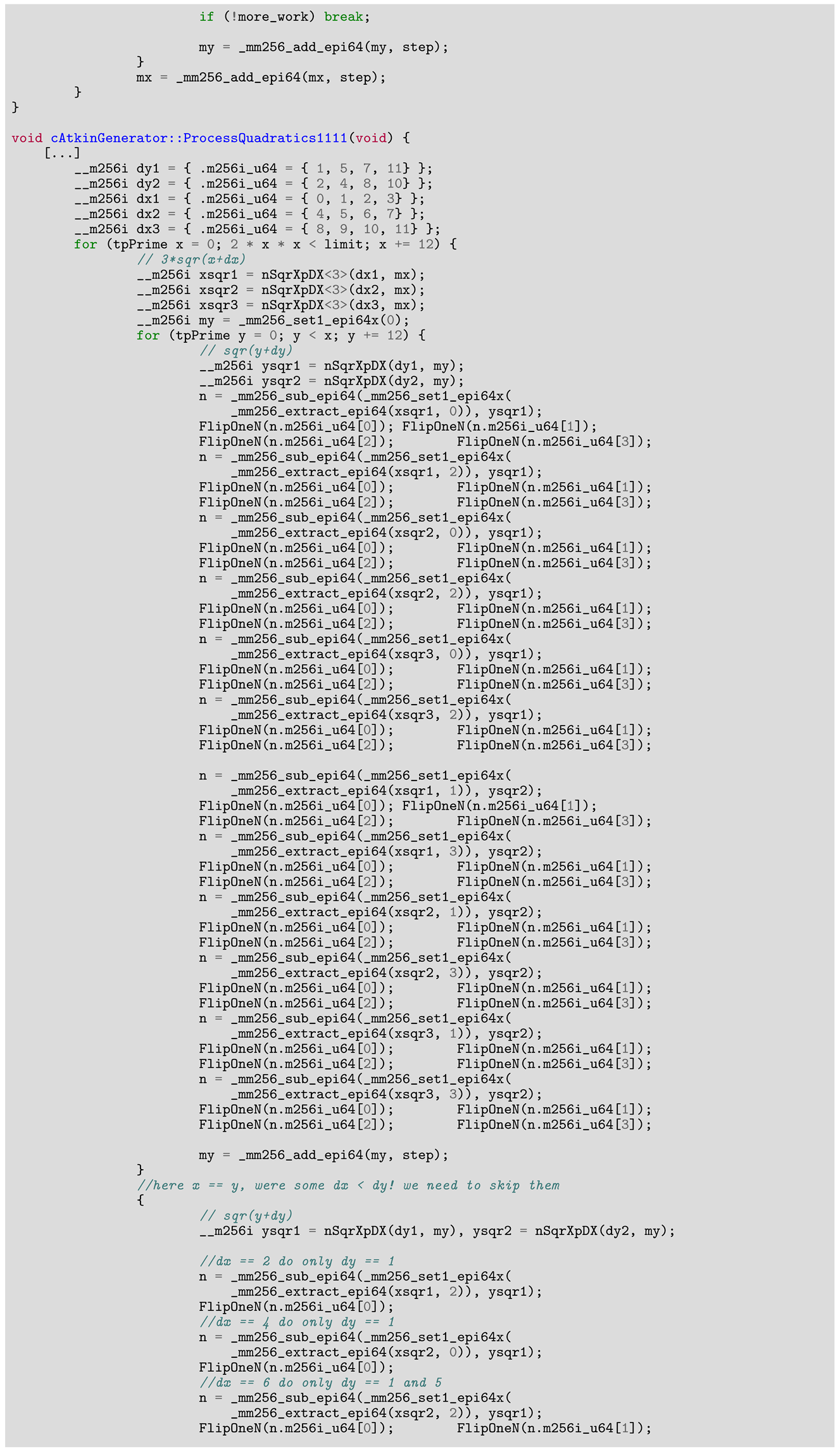
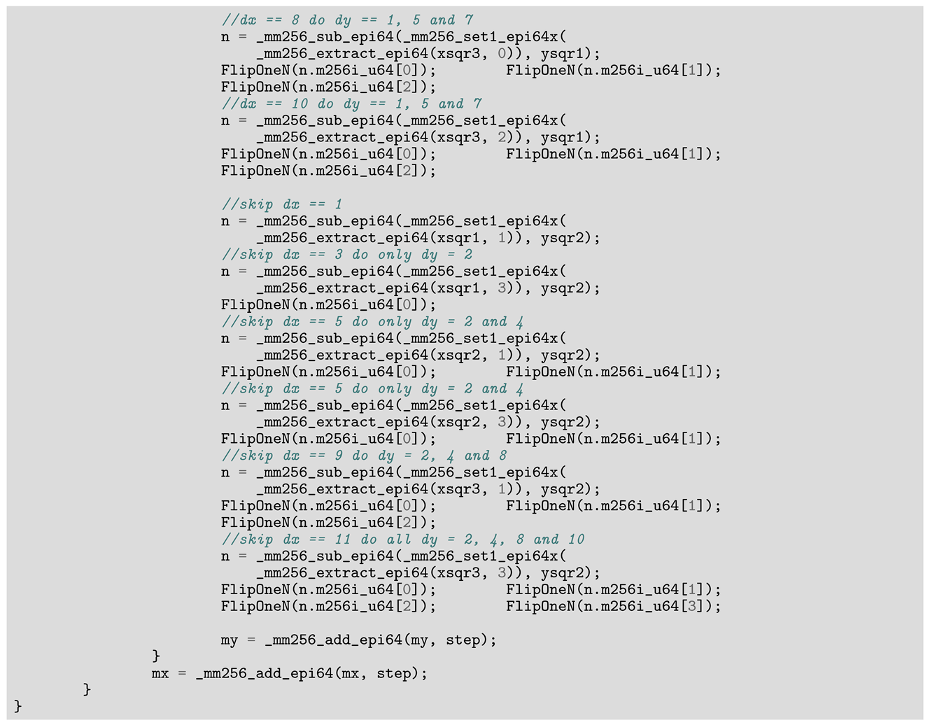
This time around, the performance went up from 3600 ms to 3300 ms, a net win. Similar methods for the other three values can be found in Appendix A. This SIMD approach will reduce the value from 3600 ms to 2750 ms. Considering that 600ms is actually spent in the last phases, not optimized with SIMD, the actual speed up is from 3000 to 2150—roughly 850 ms, almost a 30% gain.
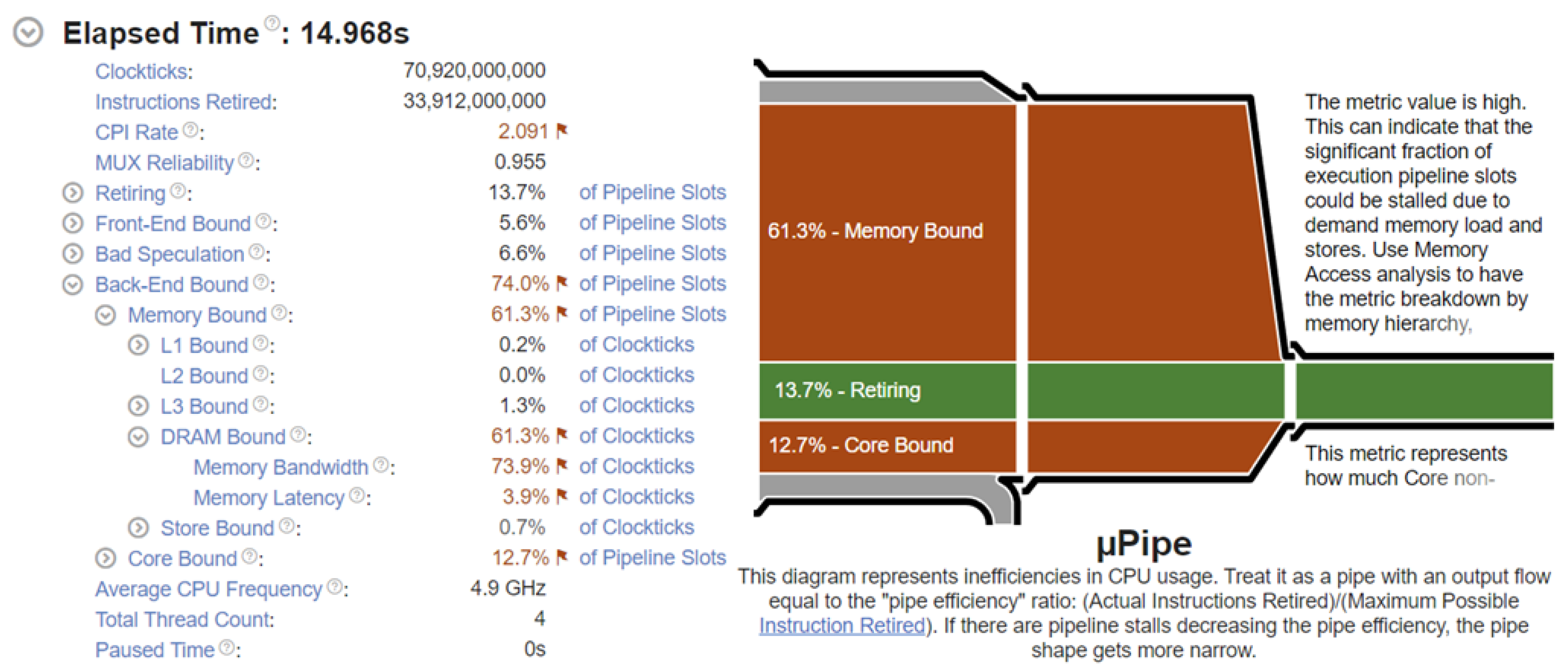
Why only 30%, when we should gain much more, as we process now four values per instruction? Because sieving is not really the best scenario for SIMD; AVX, SSE, etc., were designed to work on data organized as vectors and to perform heavy arithmetical operations, not move data around. In our case, data are scattered in memory, so we have to use a lot of scalar ops. Also, we need to manipulate some individual elements, which is not the best usage of vector instructions and will seriously slow down the sprint. On the other hand, if you mix scalar and vector instructions that have minimal data dependencies, you may get the CPU to process even more data in parallel, like here with our FLIP operations that are quite independent, so the vector ops will intersperse nicely in parallel, without having to wait for one another. Figure 7 shows the micro-architecture statistics; the impediment for performance is mainly the memory access pattern.
The code above could be streamlined a little with some inline methods; a good candidate is FLIP, which should be a generic inline outside the methods and pass the full _256i object, not values one by one. Nevertheless, given the fact that this is far from the best fit for AVX processing, we have to recognize the power of SIMD when used properly. And we must say that the optimizer does a pretty good job but is far less advanced for vector than for scalar operations; looking at the disassembled code, we can see here and there some unnecessary data movement in and out of registers. Writing assembler code for AVX2/512 code may obtain really impressive results.
Good SIMD code has a certain flavor; it is quite dull and repetitive, heavy on the eye, and boring. We need a lot of patience and focus to get it right. Still, in the right places, it can serve us well once we get the hang of it.

4.3. Generic Optimization, Complex Data structures, and Assembler

The discourse regarding sieve optimization can be very long, containing topics that are specific to sieving, but also a lot of other generic topics, applicable not only to sieving problems but also to other performance issues.
The domain of generic software optimization is extremely vast, so we delegated it to Appendix B, where we illustrate such an optimization journey applied to a version of Chartre’s mobile front wave [6,7]. Besides the generic approach to code optimization, the appendix includes an interesting variant of a binary heap, implemented also as a quaternary heap and optimized for the problem at hand. It has the special characteristic of being, for all practical purposes, unlimited, built on a quite efficient data structure that grows as much as required. Apart from the few optimizations specific to the mobile sieve, the most interesting aspect of that implementation is the fact that it places the head of the heap/tree outside the vector(s) representing the heap, thus greatly simplifying the associated arithmetic, which is now rigorously based on multiples of 2, and entirely avoiding various very frequent tests involving children placement/coherence.
Another generic topic addressed in Appendix B is the problem of the assembler and the efficiency of such a tool nowadays, when the optimizing compilers are very good at their job; our conclusion is that the assembler can indeed have a net positive return, but it will seldom be very significant. The performance on the specific function optimized in this way can increase by 10–20%, but the associated effort is extremely high, and the resulting code becomes very rigid and extremely difficult to debug and maintain, while the overall impact on the entire program may not be so important.
In any case, we are not suggesting that every programmer should learn assembler and code every inner loop in assembler. It is very difficult and generally not worth the effort. Translating the routine exemplified in Appendix B from C++ to assembler took double the time required for designing, writing, and optimizing the original C++ code, and debugging assembler code is quite challenging. However, where performance is critical, an expert who can handle such tasks may be required. In a 50,000-line program, those 500 lines of assembler can make a significant difference.
Contrary to the belief that one cannot write better code than an optimizer, a skilled human can usually produce superior code. Although advanced tools exist, they are niche and not typical of standard compilers. Despite this, the average programmer today does not master this skill, and that is acceptable, because the effort usually outweighs the results. We rely on optimizers for most of our code, which is sensible with the right mindset. However, the industry must be prepared to address that small percentage where assembler is necessary.
Assembler programming, though seen by some as a dying art, remains crucial in performance-critical scenarios, but only when all other alternatives are exhausted. Assembler is a tool of last resort; as in our example, there are usually some high-level algorithmic tweaks that will deliver much better return than assembler. Begin with a high-level language and exhaust all optimization possibilities before resorting to assembler.

5. Conclusions

After publishing several articles elucidating various sieving strategies and presenting important results, we tried to offer here a comprehensive compilation of generic tweaks and boosters derived from our collective experience.
We do not know if this article is a herald of a renaissance, but it can certainly be a testimony for the perseverance of a few sieving enthusiasts in an often-overlooked field. Drawing from a wealth of resurfaced wisdom and refined methodologies, we present a diverse array of strategies aimed at enhancing the efficiency, accuracy, and scalability of prime sieving algorithms. From subtle parameter adjustments to advanced algorithmic enhancements, these tweaks and boosters complement our series of articles dedicated to prime sieving as a less significant but still relevant part of our contribution to the domain and a witness to our efforts to breathe new life into prime sieving methodologies.
Despite the sparse community and the challenges we face, these endeavors will hopefully serve as a reminder of the enduring importance of prime sieving in computational mathematics. By sharing our insights and discoveries, we hope to inspire fellow enthusiasts to join us in this noble pursuit, ensuring that prime sieving continues to thrive, even in the face of common disinterest from the IT community.

Supplementary Materials

The following supporting information can be downloaded at: https://www.mdpi.com/article/10.3390/a17070291/s1.

Author Contributions

M.G.: Conceptualization, Methodology, Software, Validation, Formal analysis, Investigation, Writing—Original and Editing, Visualization; D.P.: Validation, Supervision, Project administration, Writing—Review. All authors have read and agreed to the published version of the manuscript.

Funding

This research did not receive any specific grant from public, commercial, or not-for-profit funding agencies.

Data Availability Statement

This study does not report any data.

Acknowledgments

We express our gratitude to Nirvana Popescu, Emil Slusanschi, and Vlad Ciobanu from University Politehnica of Bucharest, Computer Science Department, for their invaluable guidance and advice. Their input was decisive for the quality of this paper.

Conflicts of Interest

The authors declare no conflicts of interest.

Appendix A. SIMD

Algorithms 17 00291 i030
Algorithms 17 00291 i031
Algorithms 17 00291 i032
Algorithms 17 00291 i033

Appendix B. Optimizing the Mobile Sieve

The content of this appendix, provided here as Supplementary Materials, originates immediately before sieving became our primary focus, marking our transition from general code optimization to the specific optimization of sequential prime number generation. At that time, we were not yet knowledgeable about the history of sieving algorithms, so we believed we had discovered a new algorithm—not very efficient, but still a novelty. Later, in our efforts to explore the field’s history, we encountered Chartes’ algorithms and realized that our idea was not new. The concept of the mobile front-wave had already been introduced. Unintentionally, we had rediscovered an existing algorithm, similar to Mairson revisiting Euler’s algorithm or Bay and Hudson revisiting Singleton’s 357.
Nevertheless, the journey presented here is of interest due to the relatively detailed description of our significant efforts in optimizing the sieve, which are pertinent to Section 4 “Hard Core Optimization Techniques”. Therefore, lengthy as it is, we have included it as an appendix to this paper, even though it is not an integral part of the article itself. The appendix is quite dense, describing a convoluted path full of do’s and don’ts, which readers can explore at their own pace, potentially benefiting from a handful of noteworthy lessons to be learned from our mistakes and inspirations.

References

  1. Wood, T.C. Algorithm 35: Sieve. Commun. ACM 1961, 4, 151. [Google Scholar] [CrossRef]
  2. Nicomachus. Introduction to Arithmetic; D’Ooge., M.L., Translator; Studies. Humanistic Series; Macmillan: New York, NY, USA, 1926. [Google Scholar]
  3. Aiyar, V.R. Sundaram’s Sieve for Prime Numbers. Math. Stud. 1934, 2, 73. [Google Scholar]
  4. Helfgott, H.A. An Improved Sieve of Eratosthenes. arXiv 2019, arXiv:1712.09130[math]. [Google Scholar] [CrossRef]
  5. Chartres, B.A. Algorithm 310: Prime Number Generator 1. Commun. ACM 1967, 10, 569. [Google Scholar] [CrossRef]
  6. Charters, B.A. Algorithm 311: Prime Number Generator 2. Commun. ACM 1967, 10, 570. [Google Scholar] [CrossRef]
  7. Singleton, R.C. Algorithm 356: A Prime Number Generator Using the Treesort Principle [A1]. Commun. ACM 1969, 12, 563. [Google Scholar] [CrossRef]
  8. Singleton, R.C. Algorithm 357: An Efficient Prime Number Generator [A1]. Commun. ACM 1969, 12, 563–564. [Google Scholar] [CrossRef]
  9. Mairson, H.G. Some New Upper Bounds on the Generation of Prime Numbers. Commun. ACM 1977, 20, 664–669. [Google Scholar] [CrossRef]
  10. Gries, D.; Misra, J. A Linear Sieve Algorithm for Finding Prime Numbers. Commun. ACM 1978, 21, 999–1003. [Google Scholar] [CrossRef]
  11. Misra, J. An Exercise in Program Explanation. Acm Trans. Program. Lang. Syst. 1981, 3, 104–109. [Google Scholar] [CrossRef]
  12. Pritchard, P. A Sublinear Additive Sieve for Finding Prime Number. Commun. ACM 1981, 24, 18–23. [Google Scholar] [CrossRef]
  13. Pritchard, P. Explaining the Wheel Sieve. Acta Inform. 1982, 17, 477–485. [Google Scholar] [CrossRef]
  14. Paul Pritchard. Fast Compact Prime Number Sieves (among Others). J. Algorithms 1983, 4, 332–344. [Google Scholar] [CrossRef]
  15. Pritchard, P. Linear Prime-Number Sieves: A Family Tree. Sci. Comput. 1987, 9, 17–35. [Google Scholar] [CrossRef]
  16. Pritchard, P. Improved Incremental Prime Number Sieves; Tech. Rep.; Springer: Berlin/Heidelberg, Germany, 1994; pp. 280–288. [Google Scholar]
  17. Sorenson, J. An Introduction to Prime Number Sieves; Tech. Rep.; University of Wisconsin- Madison, Computer Sciences Department: Madison, WI, USA, 1990. [Google Scholar]
  18. Sorenson, J. An Analysis of Two Prime Number Sieves; Tech. Rep.; University of Wisconsin- Madison, Computer Sciences Department: Madison, WI, USA, 1991. [Google Scholar]
  19. Sorenson, J.; Parberry, I. 2 Fast Parallel Prime Number Sieves. Inf. Comput. 1994, 114, 115–130. [Google Scholar] [CrossRef]
  20. Sorenson, J. Trading Time for Space in Prime Number Sieves; Tech. Rep.; Springer: Berlin/Heidelberg, Germany, 1998; pp. 179–195. [Google Scholar]
  21. Atkin, A.O.L.; Bernstein, D.J. Prime Sieves Using Binary Quadratic Forms. Math. Comput. 2003, 73, 1023–1030. [Google Scholar] [CrossRef]
  22. Ghidarcea, M.; Popescu, D. Prime Number Sieving—A Systematic Review with Performance Analysis. Algorithms 2024, 17, 157. [Google Scholar] [CrossRef]
  23. Ghidarcea, M.; Popescu, D. Sieve of Atkin Revisited. Sci. Bull. Univ. Politeh. Buchar. 2024, 86, 15–26. Available online: https://www.scientificbulletin.upb.ro/rev_docs_arhiva/rezfd9_854826.pdf (accessed on 11 June 2024).
  24. Ghidarcea, M.; Popescu, D. Static Wheels in Fast Sieves. J. Control Eng. Appl. Inform. 2024, 26, 36–43. [Google Scholar] [CrossRef]
  25. Walisch, K. Primesieve. 2024. Available online: https://github.com/kimwalisch/primesieve (accessed on 11 June 2024).
  26. Oliveira e Silva, T. Fast Implementation of the Segmented Sieve of Eratosthenes. 2015. Available online: https://sweet.ua.pt/tos/software/prime_sieve.html (accessed on 11 June 2024).
  27. Seizert, C. CUDASieve. 2024. Available online: https://github.com/curtisseizert/CUDASieve (accessed on 11 June 2024).
  28. Muła, W.; Kurz, N.; Lemire, D. Faster Population Counts Using AVX2 Instructions. Comput. J. 2017, 61, 111–120. [Google Scholar] [CrossRef]
  29. Bernstein, D.J. Primegen. 1999. Available online: https://cr.yp.to/primegen.html (accessed on 11 June 2024).
  30. Flammenkamp, A. Sieve of Eratosthenes. 1998. Available online: https://wwwhomes.uni-bielefeld.de/achim/prime_sieve.html (accessed on 11 June 2024).
  31. Walisch, K. Speaker: Kim Walisch. 2003. Available online: https://primzahlen.de/referenten/Kim_Walisch/index2.htm (accessed on 11 June 2024).
Figure 1. Normal versus vertical sieves.
Algorithms 17 00291 g001
Figure 2. Sieving process diagram.
Algorithms 17 00291 g002
Figure 3. Normal j distribution.
Algorithms 17 00291 g003
Figure 4. Transposed approach for j distribution.
Algorithms 17 00291 g004
Figure 5. Disassembled loop code.
Algorithms 17 00291 g005
Figure 6. Valid tuples for Atkin.
Algorithms 17 00291 g006
Figure 7. Micro-architecture statistics for SIMD SoA.
Algorithms 17 00291 g007
Disclaimer/Publisher’s Note: The statements, opinions and data contained in all publications are solely those of the individual author(s) and contributor(s) and not of MDPI and/or the editor(s). MDPI and/or the editor(s) disclaim responsibility for any injury to people or property resulting from any ideas, methods, instructions or products referred to in the content.