Automatic Optimization of Deep Learning Training through Feature-Aware-Based Dataset Splitting

Abstract

The proliferation of classification-capable artificial intelligence (AI) across a wide range of domains (e.g., agriculture, construction, etc.) has been allowed to optimize and complement several tasks, typically operationalized by humans. The computational training that allows providing such support is frequently hindered by various challenges related to datasets, including the scarcity of examples and imbalanced class distributions, which have detrimental effects on the production of accurate models. For a proper approach to these challenges, strategies smarter than the traditional brute force-based K-fold cross-validation or the naivety of hold-out are required, with the following main goals in mind: (1) carrying out one-shot, close-to-optimal data arrangements, accelerating conventional training optimization; and (2) aiming at maximizing the capacity of inference models to its fullest extent while relieving computational burden. To that end, in this paper, two image-based feature-aware dataset splitting approaches are proposed, hypothesizing a contribution towards attaining classification models that are closer to their full inference potential. Both rely on strategic image harvesting: while one of them hinges on weighted random selection out of a feature-based clusters set, the other involves a balanced picking process from a sorted list that stores data features’ distances to the centroid of a whole feature space. Comparative tests on datasets related to grapevine leaves phenotyping and bridge defects showcase promising results, highlighting a viable alternative to K-fold cross-validation and hold-out methods.

1. Introduction

In recent years, the proliferation of classification-capable artificial intelligence (AI) across a wide range of domains (e.g., civil engineering [1], agriculture [2], medicine [3,4,5], aeronautics [6], footwear retail [7], etc.) has been of outstanding importance for the digitalization of knowledge among vanishing professionals with particular sets of relevant skills, leading to the automation of workflows, time-effective decision support, and the dynamization of business models, among many other benefits. Supporting the success of this family of computational approaches are several artificial neural network architectures of distinct complexities that have been proposed over time by the technical-scientific community—e.g., VGG [8], ResNet [9], Xception [10], within the scope of deep learning—with the goal of providing different strategies to reach inference models of increasingly better performances, which are typically assessed against unseen data [11]. Among the perceived challenges is the need to mitigate potential overfitting, which affects models of higher complexity more severely [12]. Therefore, employing best-practices to find the proper balance between generalization capabilities and biases contributes to the achievement of more suitable inference capabilities. One of these practices consists of finding adequate training data arrangements to ensure harmonization, configured by a balanced distribution of examples per class/label, representativeness, diversity, among other aspects. In that regard, the data splitting process for setting up datasets is crucial for the achievement of reliable and consistent models [13].

In the dataset splitting context, there are different techniques [14]. Currently, two methods are widely used for this purpose: K-fold cross-validation (KFCV) and hold-out validation (HO) [15,16,17,18]. These traditional approaches pose some issues, not only in terms of demanding both computational time and processing resources, but also because they do not always ensure the exploration of models’ full inference potential (or nearly close to that golden rate). Other eventual drawbacks include decompensations that may prevent the matching of features between training and validation examples, and even lead to unrepresentative performance assessments while testing the models against unseen data, especially in cases wherein heterogeneity is a prevalent characteristic—for example, with the inclusion of many classes and/or noisy backgrounds. In cases wherein the datasets are reduced, the division can result in subsets composed of only a few samples, impacting the effectiveness of training or evaluation. If the dataset is unbalanced, and if certain classes or categories are underrepresented in the training, validation, or testing subset, the model may not learn accurately. Design patterns [19] may not work in such scenarios either. While rebalancing by oversampling may induce bias for decompensated classes, doing it by underfitting can lead to a substantial loss of problem representation.

In this study, in contrast with conventional dataset split methodologies, two one-shot techniques are proposed and compared. Their primary focus is on achieving feature-based balanced datasets, aiming to mitigate the trial-and-error orientation underlying traditional subdivision approaches. More specifically, a lightweight feature-aware exploration strategy was conceptualized and developed to automatically and expeditiously organize data towards achieving uniform feature distribution, with the particular goal of assessing the impact of evenly distributing diversity in imagery characteristics on deep learning (DL) models’ convergence. Tests made to evaluate the proposed strategies, considering two datasets with distinct contexts (grapevine leaves for phenotyping determination and bridge defects for the identification of degradation factors) demonstrated very promising results in comparison to the KFCV and HO techniques.

Regarding the structure, besides this introductory section, the remainder of the paper is organized as follows: Section 2 will address the related work; Section 3 covers the material and methodology; Section 4 presents the experimental results, followed by Section 5, which provides a summary discussion, main conclusions and some future directions.

2. Related Work

Machine learning algorithms’ tasks include extracting features from data and constructing effective prediction models. Within this operational line, the primary objective is to create computational models that not only excel humans in making accurate predictions but also demonstrate a robust ability to generalize to new/unseen data. One of the factors that affect the model’s generalization performance is the binomial size/quality of the training, validation, and testing subsets; another one is the data arrangement, carried out through proper division. Highlighting the importance of appropriate data splitting, various statistical sampling methods for data splitting have been proposed [20].

Fox et. al [21] used both the KFCV and normal split techniques to divide the ITEC LapGyn4 Gynecologic Laparoscopy Image Dataset [22] and employed them to classify the images using a convolutional neural network (CNN) model and scale-invariant feature transform (SIFT) classification. Their results show better performance for the KFCV using a CNN. A feature-weighted sampling method was proposed in [23] to optimize the split of the dataset. In this work, firstly, a division of the full dataset into several subsets using the modified R-value-based sampling (RBS) [24] was carried out. Then, the distances of each set to the whole dataset were computed to obtain a similarity score, and the one with the smallest distance was chosen. Eliane [25] employed different methods to split the dataset into training/test sets, including KFCV, sample set partitioning based on joint x–y distance (SPXY), Kennard–Stone (KS), and a random sampling algorithm. The use of Pearson correlation scores (PCSs) for comparison allowed for ranking the performance of these approaches from best to worst, as follows: KFCV, SPXY, and KS. An algorithm for performing stratified KFCV with a focus on similarity-based sample splitting was developed by Farias et al. [26]. First, they select a pivot sample from each label group that is most similar to other samples within the same label group. Afterward, the algorithm identifies additional samples that are most similar to the “pivot” sample. They employed different similarity functions, including Cityblock, Chebyshev, Euclidean, cosine, and correlation, deploying different classifiers: nearest neighbors (KNN); random forest (RF) classifier with 100 trees; support vector machine (SVM); and multilayer perceptron (MLP). Their results showed the better performance of the proposed algorithm over the normal KFCV when using the correlation similarity function. It is worth mentioning that the difference between the accuracies of different similarity functions was almost 1%. Nurhopipah et al. [27] compared four dataset splitting techniques for face classification tasks: random sub-sampling validation, bootstrap validation, KFCV, and Moralis Lima Martin validation (MLMV). They concluded that KFCV provides a more stable performance, with higher accuracy. The KFCV method was, once again, employed in [28] to partition brain image samples for tumor diagnosis, using the SVM algorithm. In this work, different kernels of the SVM were used. In [29], KFCV, with K = 10, was applied to split a vegetation dataset into training and validation subsets and, subsequently, build different classifiers—k-nearest neighbors, Gaussian naive Bayes, random forests, SVM, and multilayer perceptron—capable of performing vegetation physiognomic classification. Inside the cross-validation loop, they performed a univariate statistical test (ANOVA F-value) between physiognomic classes and the features in the training set to select the best-scoring features from the training set. A higher accuracy (81%) was verified for random forests.

Varma and Simon [30] used both normal and nested KFCV and showed that the nested one can be considered a nearly bias-free method. Vabalas et al. [31] used the train/test split, normal, nested, and partially nested KFCV to split the dataset, as well as an SVM and a logistic regression classifier to distinguish autistic from non-autistic individuals. In their experiments, the train/test split and nested KFCV approaches produced robust performance. Kahloot et al. [32] developed a technique named “Algorithmic splitting”. They used, firstly, the Umap technique for dimension reduction and then two different clustering methods, including hierarchical density-based spatial clustering of applications with noise (HDBSCAN) [33] and gaussian mixture models (GMM) [34]. The distances of data points to the mean were computed using Chebyshev’s inequality bound [35]. For each cluster, they calculated the mean (μ) and standard deviation (σ) of the data points’ positions. Then, the algorithm defines different ranges based on μ and σ, which include a “median range” (within 1 standard deviation from μ), an “extreme range” (beyond 2 standard deviations from μ), and a “quantile range” (between median and extreme ranges). For each sub-dataset size (training, validation, testing with sizes of 70%, 20%, and 10%, respectively), the algorithm samples data points from the defined ranges according to specified percentages and experiments with different rates of selection for each range to train models based in VGG [8], ResNet [9], and Inception [36]. The optimal percentages were 55%, 35%, and 10% out of the median, extreme, and quantile ranges, respectively. For comparison purposes, they also split the dataset using random sampling. They concluded that the hierarchical density-based spatial clustering of applications with noise (HDBSCAN) outperforms the GMM with the algorithmic split.

To split the dataset, Doan et al. [37] first divided each class into clusters using HDBSCAN and then applied a stratification technique to select data from each cluster for the train/test set. They also used random sampling, stratified sampling, stratified cross-validation, and bootstrapping techniques as data splitting techniques and compared the results with their approach, which proved to outperform the others for all the trained models (MLP, SVM, RF, XGBoost).

Resampling, including normal, repeated, nested, leave-one-out KFCV, was used by [38] to split a dataset for training different ML algorithms (linear regression, Bayes ridge regression, ridge regression, LASSO regression, K-nearest neighbors, CART decision trees, support vector machines regression—SVMR, extreme gradient boosting, gradient boosting, random forests, and extra trees) to predict profits in olive farms. Their results presented a better performance for SVMR compared to the others, and the resampling technique outperformed the other splitting techniques. Huang et al. [39] split a dataset randomly, in a traditional fashion, with a ratio of 4:1 for training and validation, respectively, for their objective, which was using the U-Net for segmentation and AlexNet, VGG16, VGG19, ResNet-50, Inception V3, and Xception for classification.

In specific contexts, such as agriculture, traditional dataset splitting is the preferred option to be used [40,41,42], even in limited dataset conditions, as can be verified in [43], which proposes the use of KFCV to split datasets to feed decision tree, random forest, gradient boosting, and SVM models, aiming at tomato crop yield prediction, based on certain inputs (soil properties, applied fertilizers, and weather conditions). Optuna [44] employed a feature selection technique and, in the end, better performances were found for gradient boosting and SVM. The same tendency of using traditional dataset splitting techniques can be verified in the construction field [45].

From the works addressed above, one can infer that data-based features for setting up ML/DL models are of key importance. In this context, two main steps can be identified: (a) feature extraction, which can be done using specific layers of consolidated CNN architectures, such as VGG16—widely known for its capabilities in artificial deep vision tasks [46,47,48]—benefiting from ImageNet [49] weights; and (b) dimensionality reduction, achievable through techniques such as, for example, principle component analysis (PCA), which is also capable of retaining the relevant variance of the data to preserve its intrinsic characteristics [50,51,52].

To sum up, most of the data splitting-related works rely on techniques that can be computationally burdensome and time-consuming, such as KFCV. In contrast, single passages of HO techniques are likely to lead to uncalibrated datasets in terms of features—it is hypothesized that the presence of elements in training images that, if missing in the validation subset, cannot be confirmed and consolidated—potentially constraining the exploration of the full potential of the models. Therefore, this study proposes methods to work around the identified issues. The goal is to balance features during the training, validation, and test stages. Further details will be explained in the following section.

3. Materials and Methods

This section presents the research approach, detailing the methodical preparation of materials and outlining the methodologies employed in this study. It covers the contextualization of the raw data used for experimentation purposes, as well as specific methods applied for optimizing the dataset splitting techniques.

3.1. Imagery Used for the Empirical Assessment of the Proposed Dataset Splitting Methodology

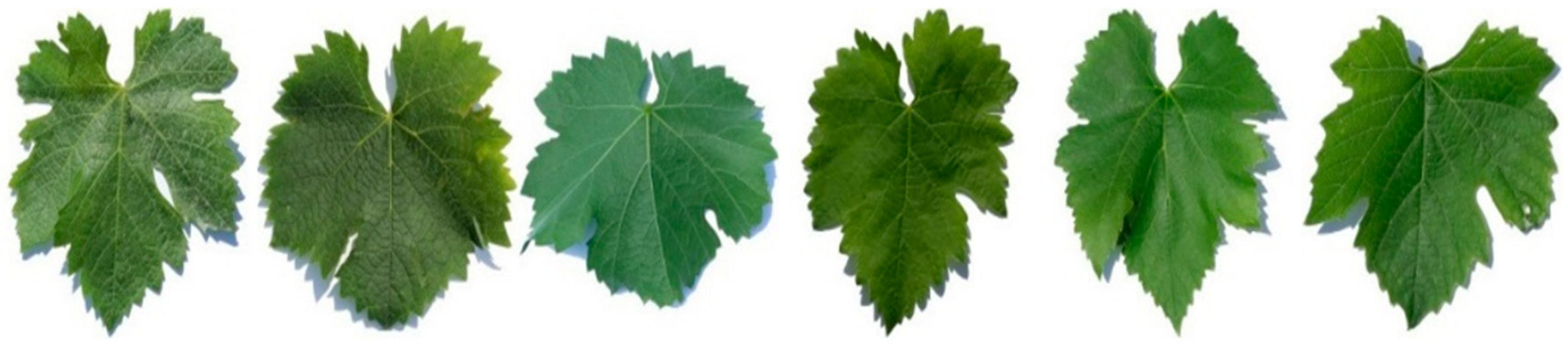
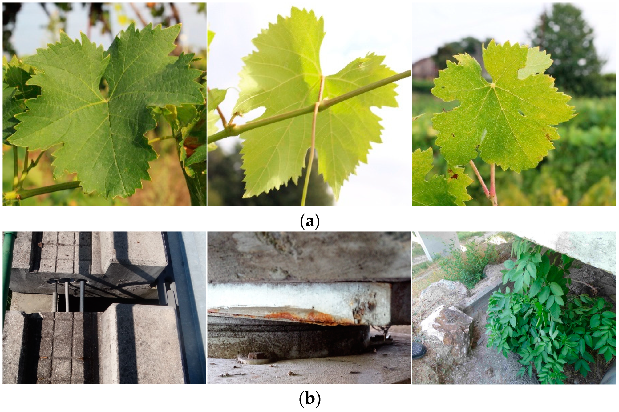
A couple of distinct groups of imagery involving differentiated contexts are considered to perform empirical experiments on the proposed feature-aware dataset splitting methodology. The first image group, described in [2], within the context of viticulture, is composed of 6 different varieties (Figure 1), summing up a total of 480 images. The varieties involved in this image group are the following: Touriga Nacional, Tinto Cão, Códega, Moscatel, Tinta Roriz, and Rabigato. In terms of acquisition procedure, weekly between 4 May and 31 July 2017, one leaf was picked from the same two previously selected plants of each grapevine variety, put on top of a white sheet of paper (background), and photographed (in the field) without any artificial lighting, using a Canon EOS 600D, equipped with a 50 mm f/1.4 objective lens (Canon, Ota, Tokyo, Japan). For the sake of variability, data collected on cloudy days and in sunny late afternoons was also included. It is worth noting that leaf acquisition and labeling were supported by domain experts.

Table 1. Distribution of classes and their respective sizes within the grapevine leaves imagery.

Class Name	Códega	Moscatel	Rabigato	Tinta Roriz	Tinto Cão	Touriga Nacional
Size	80

presents the distribution of examples per class, more specifically 80 images evenly assigned.

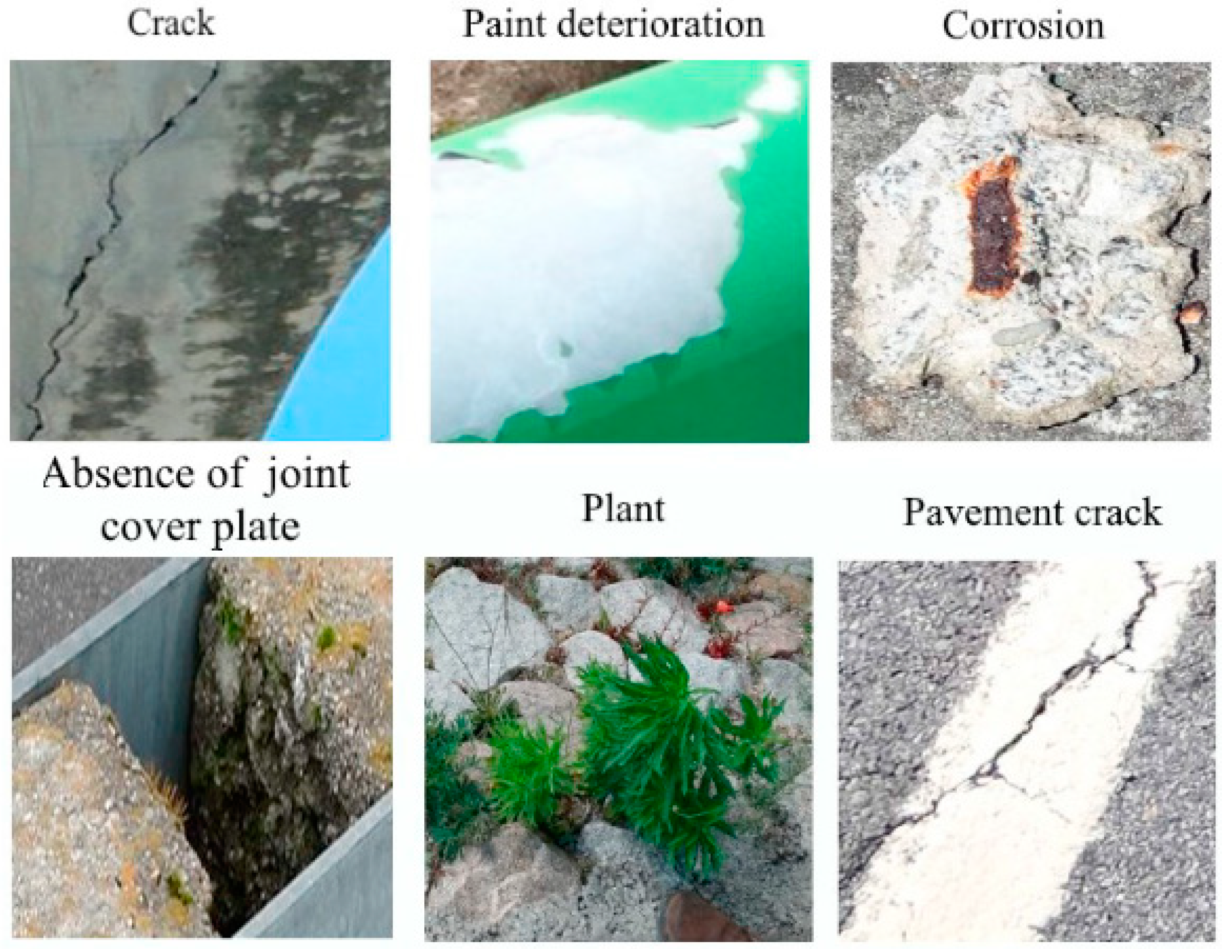
The second image group regards the context of bridge defects. This collection was created by capturing photographs of various bridges using a handheld camera and a mobile phone, resulting in a set of images with a diverse range of sizes and resolutions. Afterward, each image was manually labeled using a tool called LabelImg [53] and attributed to one of the six groups representing defect types: paint deterioration, plant, absence of joint cover plate, cracks, pavement crack, and peeling on concrete (Figure 2). In total, 2400 images were labeled. However, a pruning operation to remove unusable data had to be carried out, resulting in a final set of 1872 images. Civil engineers possessing technical expertise in the relevant domain both participated actively in the direct image acquisition process and provided support for the labeling procedures.

The distribution of classes in this dataset is illustrated in

Table 2. Distribution of classes and their respective sizes within the bridge defects imagery.

Class name	Absence of Joint Cover Plate	Cracks	Paint Deterioration	Pavement Crack	Peeling on Concrete	Plant
Size	149	461	406	523	101	232

. The “pavement crack” class is largest, with 461 images, while the “peeling on concrete” class is the smallest one, containing 101 images. This dataset showcases an uneven distribution of data among the classes.

Having both balanced and unbalanced datasets allows a more realistic evaluation of the splitting techniques under comparison.

3.2. Complementary Imagery for Extended Assessments—Models Inference Consistency and Attention Map Analysis

Two other grapevine and bridge defects external datasets were included in this study (Figure 3), envisaging an extended assessment that focuses on the following aspects: (a) the model prediction consistency over data that are characteristically different from the ones used for training; (b) CNNs attention maps-based metrics for a richer interpretation of the trained models.

Within the vineyard context, another dataset of 12 grapevine varieties was considered, based on imagery captured in a natural background—Códega, Malvasia Fina, Malvasia Preta, Malvasia Rei, Moscatel (Galego), Mourisco Tinto, Rabigato, Tinta Amarela, Tinta Barroca, Tinta Roriz, Tinto Cão, and Touriga Nacional. It resulted from a campaign that took place from 17 July to 20 September 2019, in intervals of 2 weeks, to collect 888 images of leaves, slightly unbalanced in terms of classes distribution. As with the previous grapevine group, lighting conditions were mostly influenced by direct solar incidence, occurring between 1 PM and 3 PM. However, both cloudy and sunny late afternoon illumination conditions were also considered to complement imagery variability. The acquisition equipment was the same as the one previously described for the 6-class grapevine dataset, i.e., a Canon EOS 600D camera. In the scope of this study, a pruning operation was carried out to ensure that the labels/classes of both grapevine datasets involved matched with each other, and a total of 10 samples per class were randomly considered.

The creation of the external assessment set for the bridge defects followed a similar methodology, outlined in the first collected set of this domain. Utilizing the same equipment and conditions, images were captured with a handheld camera and a mobile phone to cover the six defect classes from the bridge: paint deterioration, plant, absence of joint cover plate, cracks, pavement crack, and peeling on concrete. Just like in the latter external grapevine dataset, 10 images per class were randomly selected, setting up the final bridge defects imagery used for extended assessments in this study.

In this work, formal notation is defined to represent the specific datasets as $D_n^i$, where

• D represents the dataset;
• i represents a specific dataset chosen from a set of datasets I = {bridge defects imagery (BDI), grapevine leaves imagery (GLI)};
• n represents the specific sets N = {training-validation (Tr-Val), train (Tr), validation (Val), test (Tst), and external test (Ext_Tst)}.

3.3. General Workflow

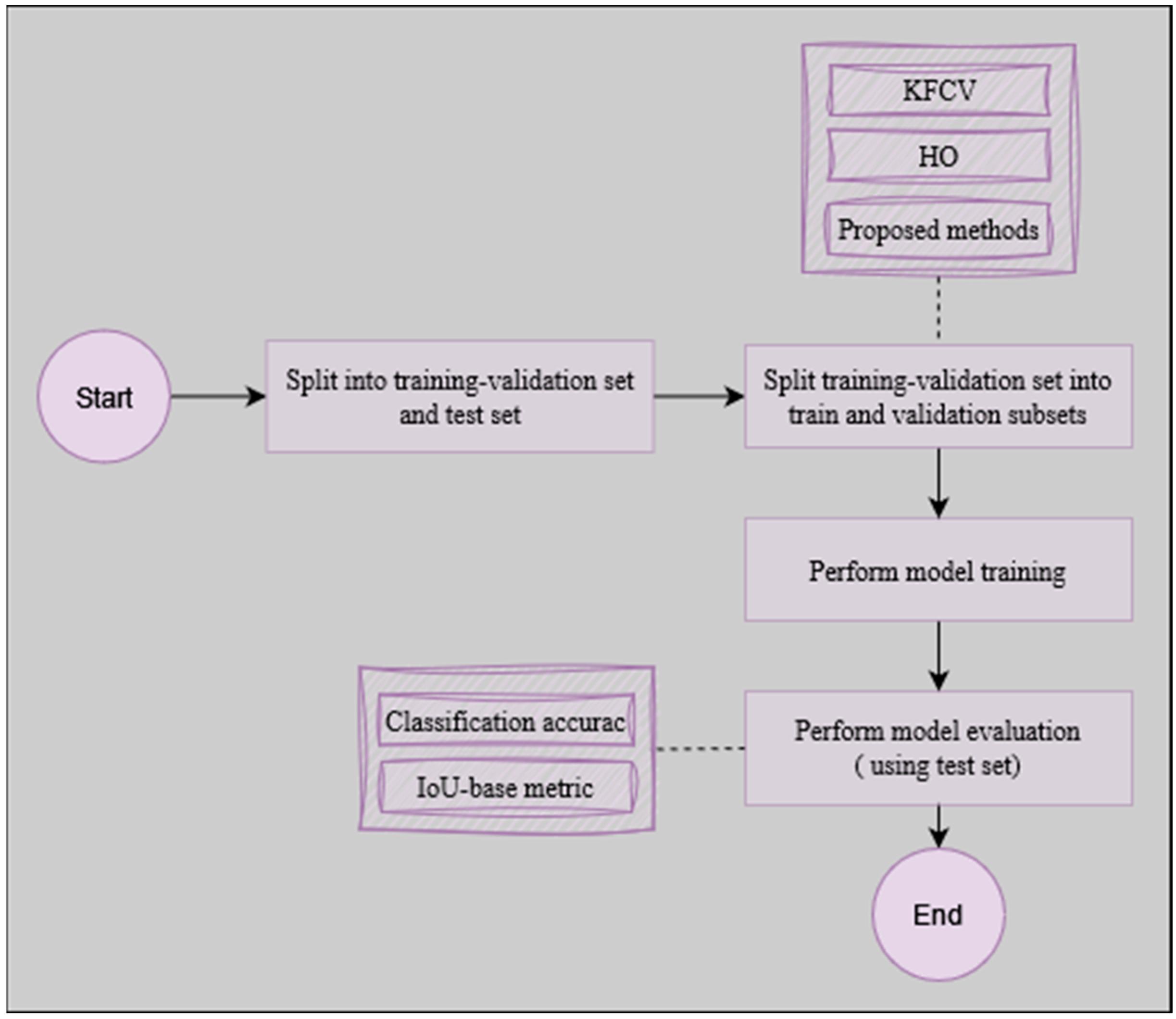
The process of model development begins with a critical step, which is the division of the original dataset into distinct subsets for training-validation and testing. This process serves as the foundation upon which the subsequent stages of model refinement and evaluation rest. The workflow of this work (Figure 4) begins by partitioning the original raw data into the training-validation and testing subsets, at a rate of 80% and 20%, respectively. Then, the training-validation subset is subdivided once again into train and validation subsets. During the evaluation step, a set of commonly used metrics is employed to assess resulting models, namely, involving accuracy and intersection over union (IOU). These metrics characterization can be found below:

• Accuracy is a fundamental metric in the field of machine learning, measures the proportion of correctly predicted instances out of the total number of instances. It is usually used to evaluate how well the model classified and predicted classes over a testing subset. More specifically, it provides an overall assessment of a model’s correctness (Equation (1)).

  $$\mathrm{Accuracy}=\frac{TP}{TP+TN+FP+FN}$$

  (1)

  where true positives (TP) and true negatives (TN) represent, respectively, the number of instances that were correctly classified as positive and negative by the model; in turn, false positives (FP) and false negatives (FN) correspond to the number of instances incorrectly classified as positive and negative, respectively.
• IOU is a spatial overlap metric commonly used in tasks involving object detection and segmentation. It quantifies the degree of overlap between the predicted regions and the ground truth regions. Specifically, IOU calculates the ratio of the intersection area between the predicted and actual regions to the union area of those regions. IOU allows the capture of the spatial alignment and precision of the model’s output in relation to the true object regions. To compute it, the most prominent attention area of CNN’s gradient-weighted class activation mapping (Grad-CAM) is used as a bounding box predictor (Equation (2)).

  $$\mathrm{IoU}=\frac{OverlapArea}{UnionArea}$$

  (2)

  where OverlapArea and UnionArea represent, respectively, the intersection and the union between ground-truth and the predicted bounding boxes of a given object of interest.

Regarding the training process, the Xception architecture is employed using Adam with Nesterov momentum (Nadam), and stochastic gradient descendent (SGD) optimizers with an initial learning rate of 1 × 10⁻³. To assure the consistency of the training conditions across all dataset splitting approaches, a set of hyperparameters is maintained across the experiments. This includes a batch size of 32, ensuring efficient training iterations; 100 training epochs; and an early stopping callback with a patience of 20 epochs. This former event monitor tracks validation accuracy and triggers in the absence of fluctuations greater than 1 × 10⁻⁴ for more than 20 consecutive epochs, indicating model stagnation. Also, a dropout regularization with a weight of 0.2 was included to make the models less prone to overfitting.

It is important to note that the hyperparameters used in the experiments were chosen based on previous work [1] and remained consistent across all training sessions. This seeks to ensure a fairer comparison and consistency in model training, by duly isolating and accommodating the main study object, i.e., the impact of varying splitting techniques.

3.4. Hardware and Software Tools

All the operations related to the deep learning models training and evaluation took place in a computer composed of the following components:

• Processor: an Intel(R) Core (TM) i7-8700 CPU 3.20 GHz 3.19 GHz (Intel Co., Santa Clara, CA, USA);
• Random access memory (RAM): 16.0 GB (Corsair, Fremont, CA, USA);
• Graphic card: NVIDIA GeForce GTX 1080, 16.0 GB (NVIDIA Co., Santa Clara, CA, USA);
• Storage: 500 SSD (Samsung Electronics, Suwon, Republic of Korea);
• Operative system: Windows 10 Pro (Microsoft Co., Redmond, WA, USA).

In terms of software, the implementation of this module was conducted utilizing Python version 3.8. The deep learning library employed in this project was TensorFlow version 2.8, strategically configured to leverage the computational power of the GPU.

3.5. Setting Up the Standards: Traditional Splitting Methodology

Two fundamental strategies commonly employed for dataset split are (i) the HO method; and (ii) the KFCV technique.

HO splitting involves partitioning the dataset into two subsets: the training set and the validation set. The training set, which usually holds most of the dataset, is used for training the models. The validation set, comprising the remaining portion, is kept separate and is used for evaluation. On the other hand, KFCV involves partitioning data into K-folds. The model is trained K times, each time using K-1 folds for training, leaving one for validation (Figure 5).

The splitting rates adopted in this work are 80% and 20% for training and validation subsets, respectively.

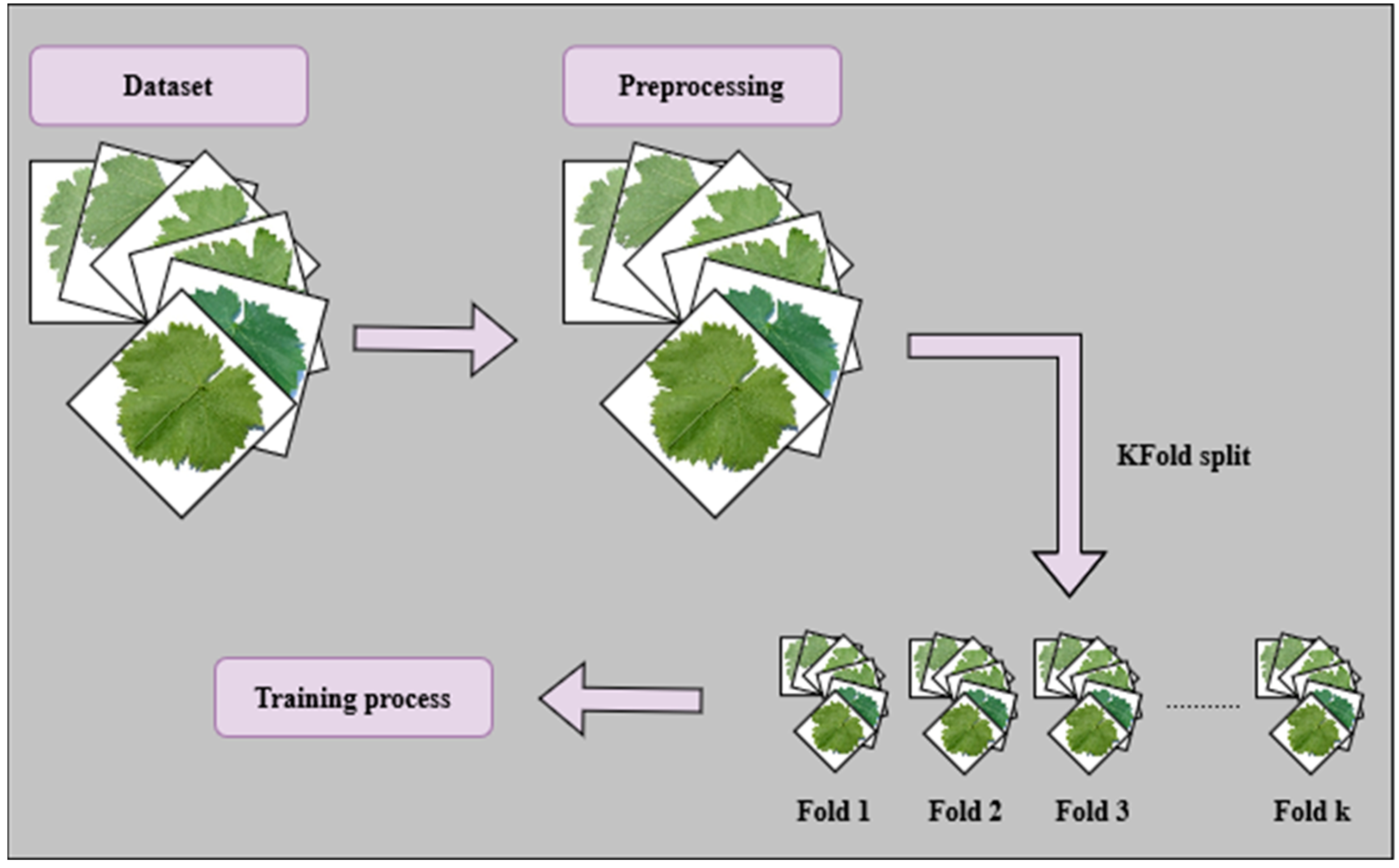
3.6. Proposed Diversity-Oriented Data Split Approaches

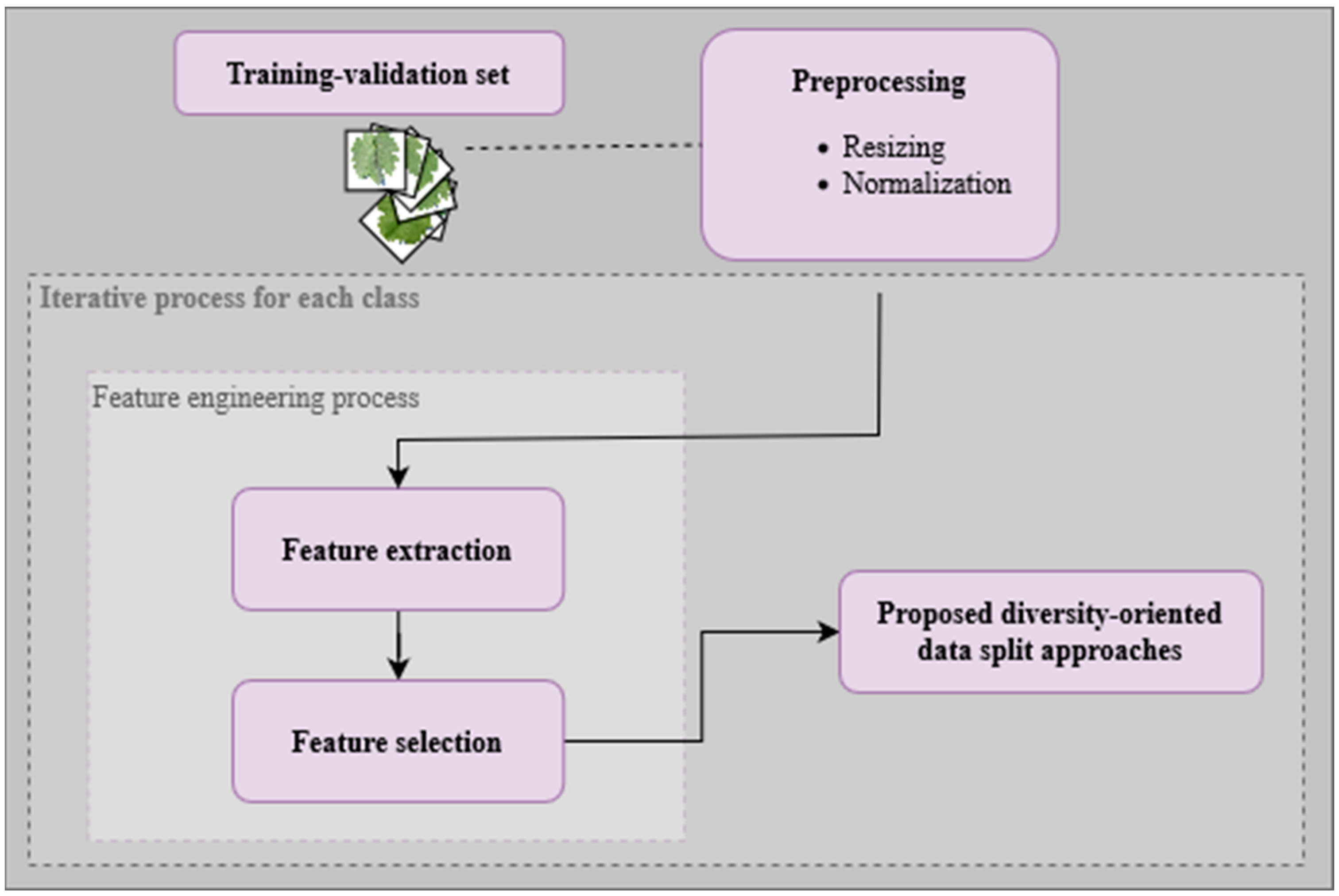
The data split approach involves the integration of two key steps: feature engineering and dataset splitting. The general workflow encompassing these steps is depicted in Figure 6.

3.6.1. Preliminary Feature Engineering

The feature engineering stage stands as the foundational step in the data preprocessing pipeline. Its primary objective is to transform input data into a more representative and informative feature space. This is achieved by extracting relevant characteristics, patterns, and representations from the data. This empowers the subsequent stages of the model to work with more meaningful inputs, leading to enhanced performance and faster convergence.

VGG16 was chosen as a robust CNN architecture for feature extraction due to its ability to effectively capture complex patterns based on deep image features. Moreover, considering the volume of classes and images that compose the two sets of raw data described previously, the extraction process occurs with due immediacy, at least, taking less than 3 s per class, depending on the hardware in use, also detailed earlier.

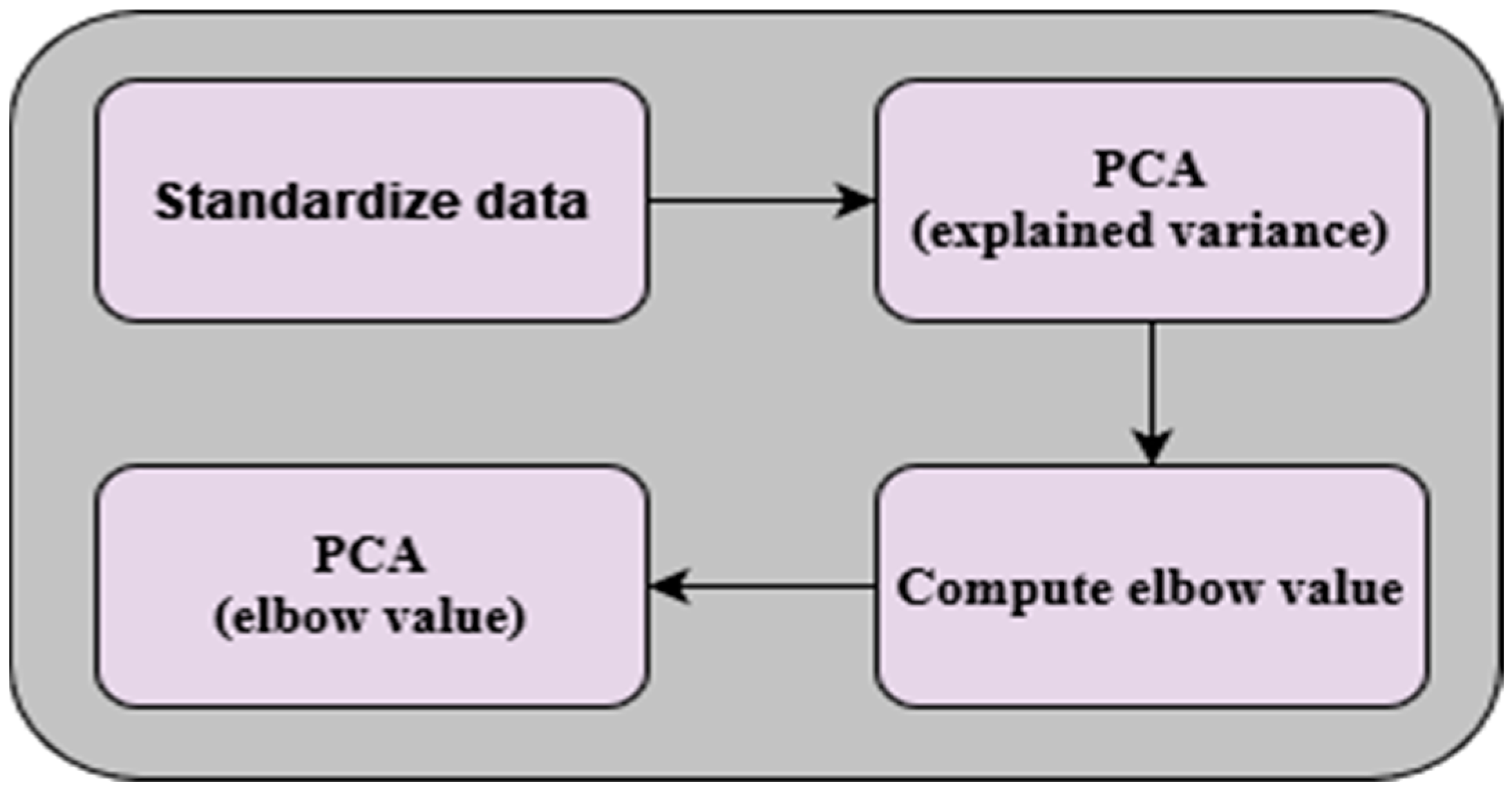
In addition, PCA was included to systematically perform dimensionality reduction upon the VGG16-based feature maps. A fundamental principle of the PCA implementation was the criterion of maintaining components that collectively explain at least 99% of the variance within the data. By keeping only those components that encapsulate the most significant information, we ensure the preservation of the essence of the dataset while simultaneously eliminating noise and redundancy. To ensure the effectiveness of PCA, a prerequisite step involved the standardization of the data, which involves transforming the variables to have a mean of zero and a standard deviation of one, preventing features with larger scales from disproportionately influencing the PCA process. To reach a functional dimensionality reduction, the selection of the final number of components is vital. To this end, the elbow value is computed by analyzing the explained variance ratio derived from PCA. The elbow value can be interpreted as the inflection point at which the marginal gain in the explained variance diminishes significantly. Once the elbow value was established, it was employed to guide the final reduction of features. Only the relevant components, as determined by the elbow value, were retained for the transformation of the data. This step resulted in the generation of a new feature space, compactly encapsulating the most valuable aspects of the original data. The implemented PCA process is depicted in Figure 7.

By combining VGG16 for robust deep features extraction and PCA for effective dimensionality reduction, a synergetic approach to grouping data by representative characteristics with reduced computational costs was achieved, standing as a key component in the proposed methodology.

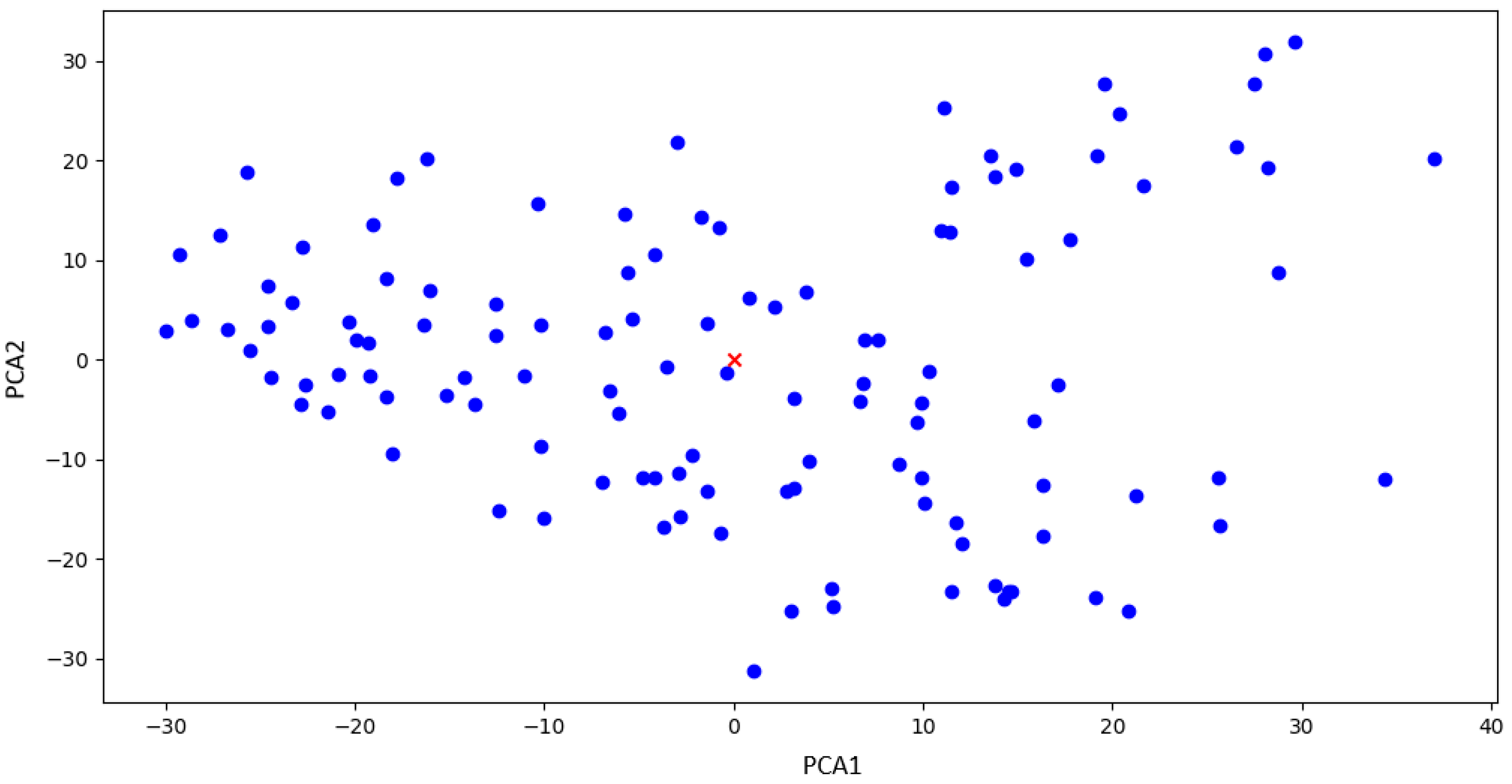
For the proposed dataset split, the centroid points of the features are computed, which will be used as a key parameter for the further processes. In Figure 8, an illustrative example of this process is provided, showcasing the centroid denoted by a distinctive red cross.

Two methods are proposed for systematic feature-aware data splitting, aiming towards diversity-oriented dataset structures: (a) feature clustering distance-based image selection (FCDIS) and (b) feature space center-based image selection (FSCIS). Both methods start by considering 80% of the $D_{Tr-Val}$ in the $D_{Tr}$ and save the remaining 20% for the $D_{Val}$.

3.6.2. Feature Clustering Distance-Based Image Selection (FCDIS)

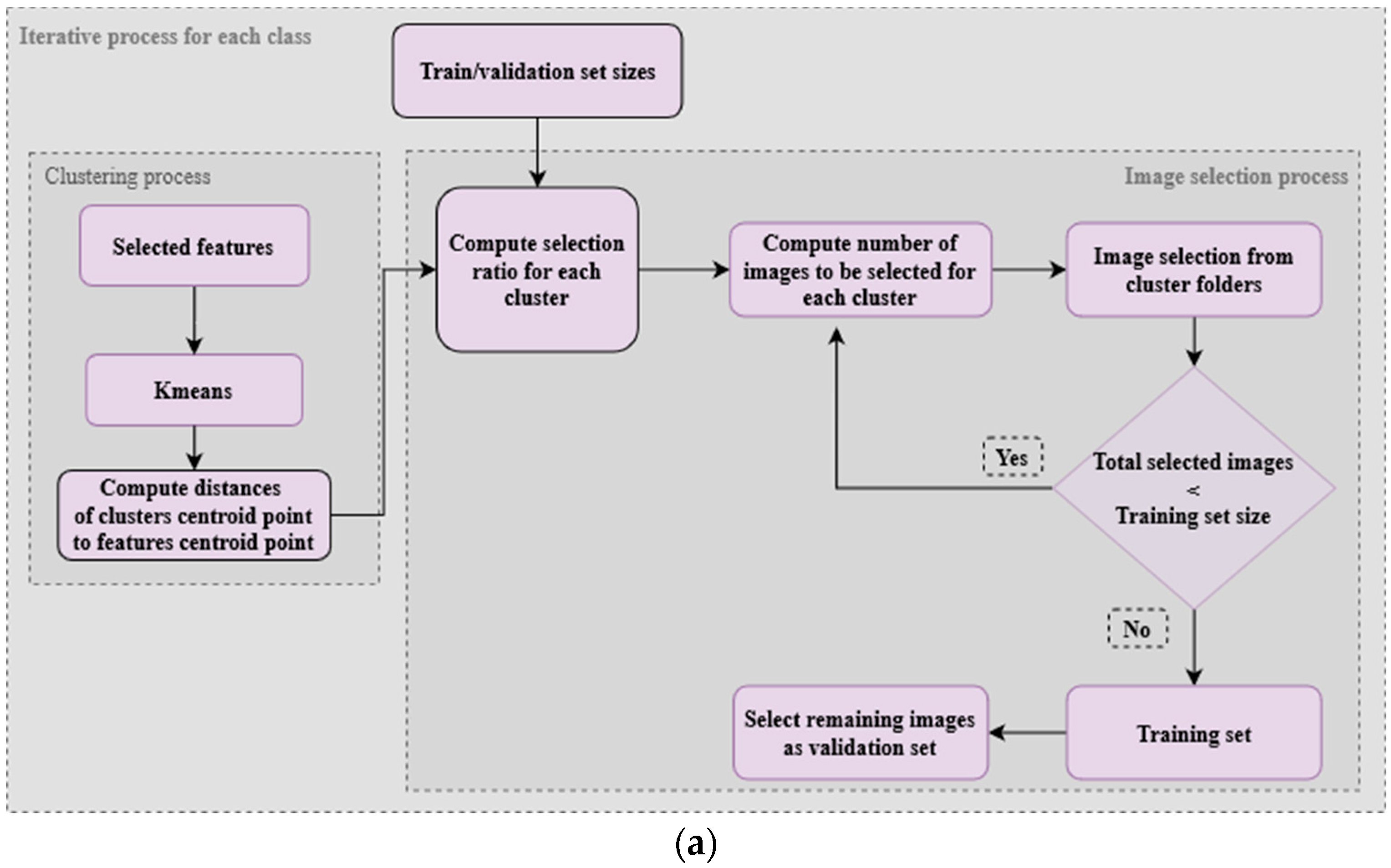
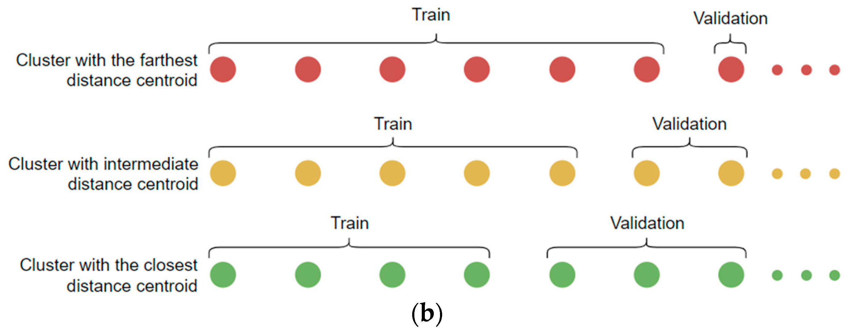
The primary step in the FCDIS method is centered on the clustering technique, where features extracted from each data class are structured using the K-means clustering algorithm. Figure 9 illustrates the process that serves as a foundation for the FCDIS splitting method, accompanied by a plot designed to provide an informative schematic representation of the divisions resulting from the application of this process.

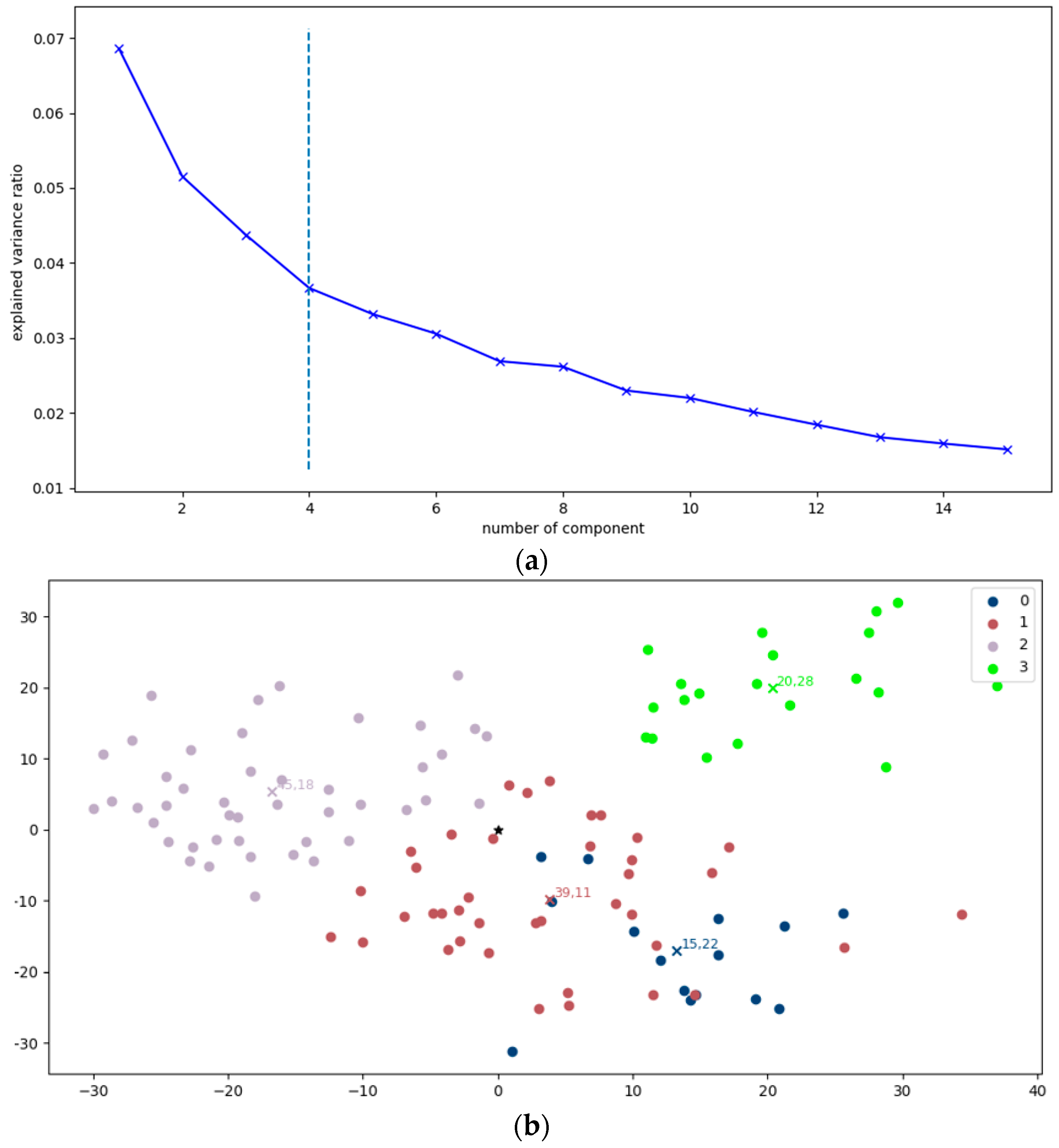
K-means partitions the feature space into K clusters based on the similarity of the deep features, aiming at the creation of distinct groups of related data points. To optimize the clustering process, a crucial step involves fine-tuning the parameter K, using a precomputed elbow value determination step (Figure 10a), aiding in the identification of the optimal number of clusters necessary to effectively segment the data within a specific class [54,55]. Then, an iterative process is employed for each class to select images for training. The essence of this selection lies in the distance ratio, wherein images positioned in farther clusters from the global centroid are accorded higher consideration. More specifically, a computation step of the distance between each cluster’s center and the center of the entire features space is carried out (Figure 10b). The latter center corresponds to the global one, denoted as $C$, which is the mean of the top-2 principal components in the reduced feature space. This distance is computed using the Euclidean distance formula:

$$Distance(c_i,C)=\sqrt{{{(c}_{ix}-C_x)}^2+{{(c}_{iy}-C_y)}^2}$$

(3)

where ${(c}_{ix},c_{iy})$ are the coordinates of the $i$-th cluster center and correspond to ${(C}_x,C_y),$ the coordinates of the global center. Then, a metric-based distance is used to determine the images’ selection size allocation for each cluster, according to the following formula:

$$ImageSelectionSize\left(c_i,\right)=\frac{Distance(c_i,C)}{\sum _{j=1}^{n}Distance(c_j,C)}$$

(4)

where $n$ represents the total number of clusters in the class. This ratio is used to determine the relative importance of each cluster in contributing images used for setting up training/validation sets. It is based on the distance of their respective center from the global center, with direct impact.

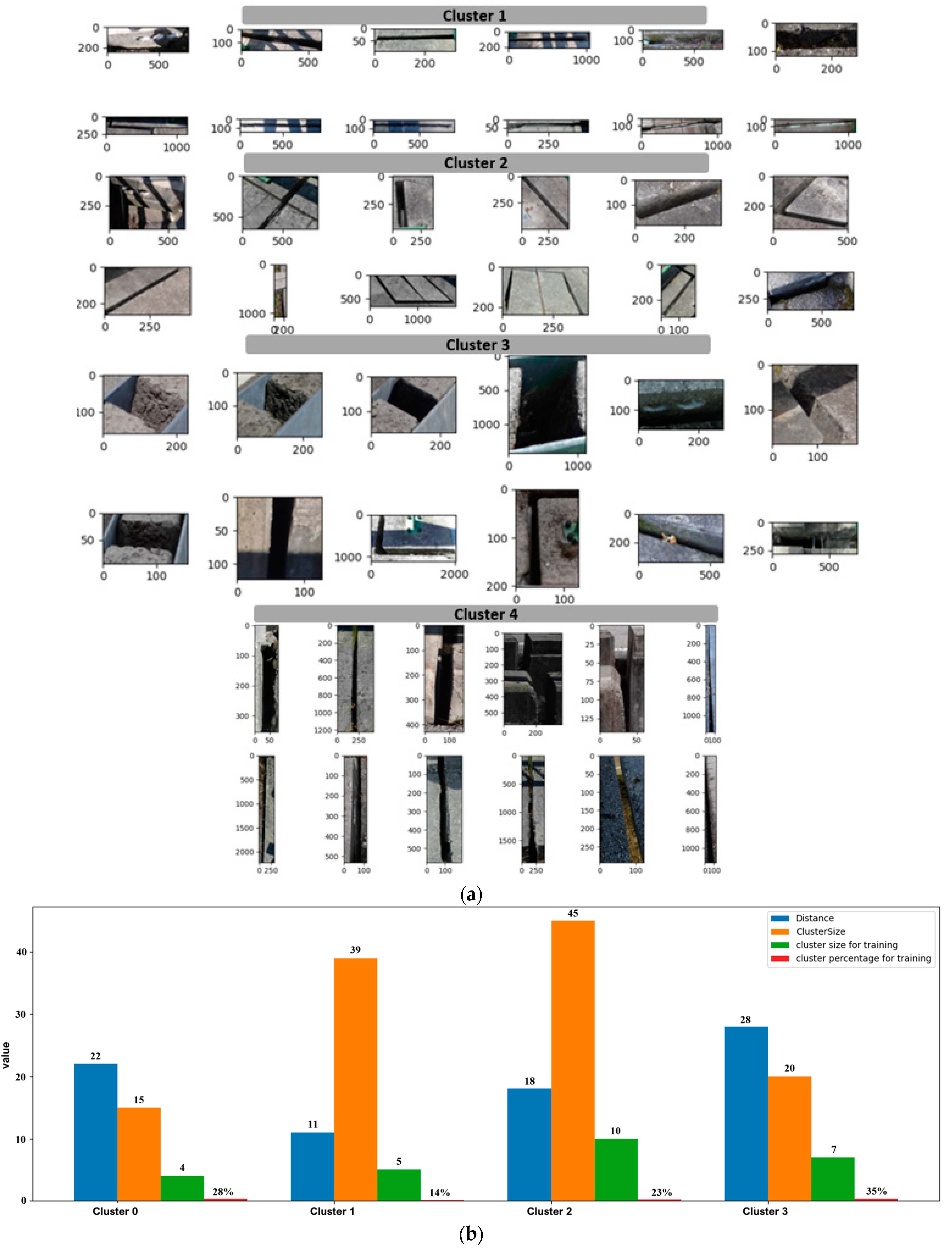
More intuitive results of the FCDIS approach can be seen in Figure 11, considering the bridge defects “absence of joint cover plate” class as an example. Upon closer examination, a noticeable visual similarity becomes apparent among images clustered together. This visual consistency proves that the clustering algorithm successfully identified and grouped images that share common features related to the “absence of joint cover plate” class. In addition, in Figure 11b, a summary of the images collected for constituting $D_{Tr}$, dependent on the distances and sizes of the clusters, is provided.

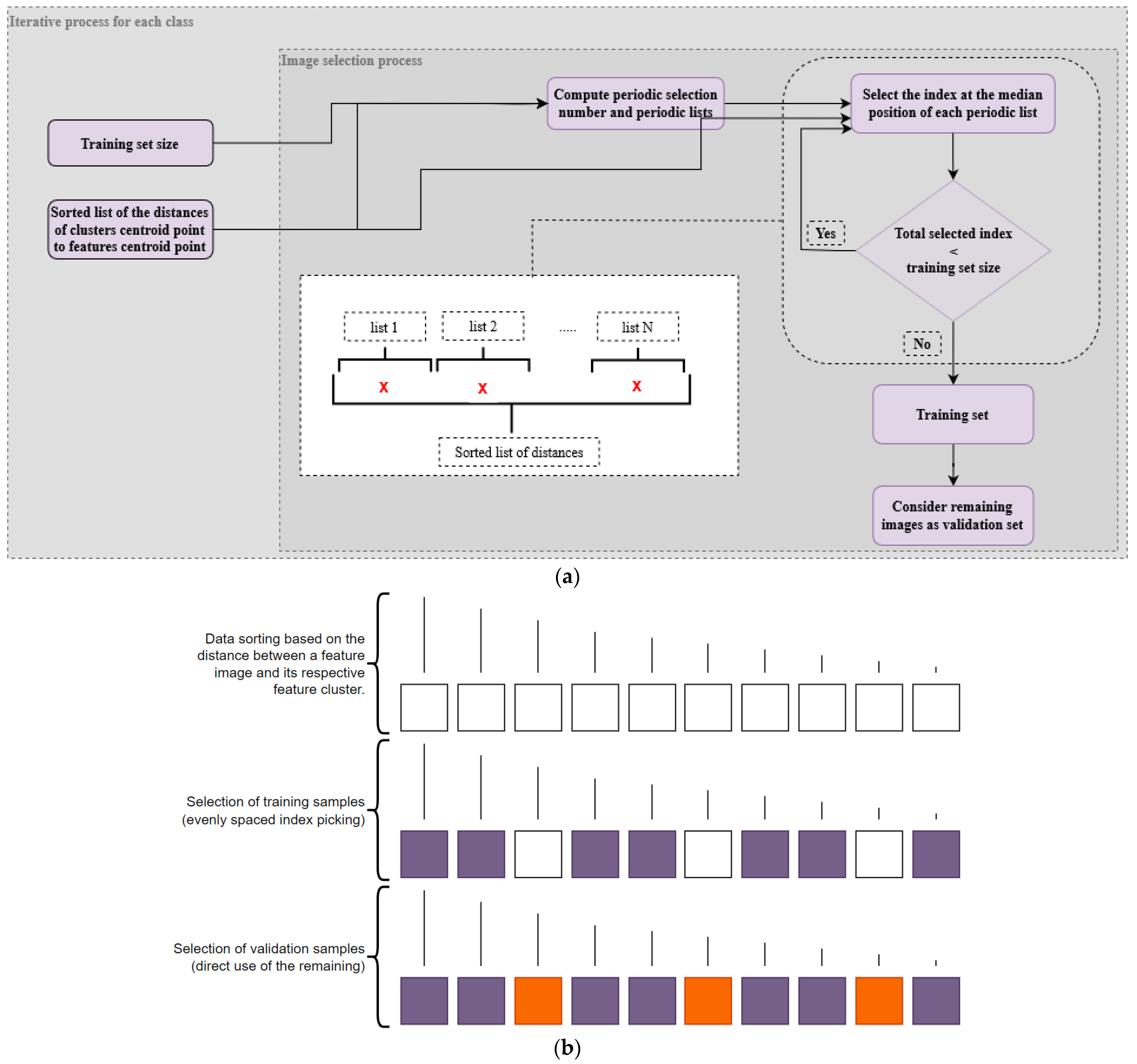
3.6.3. Feature Space Center-Based Image Selection (FSCIS)

The main objective of this approach is to partition a given distance list into multiple sub-lists, subsequently enabling the selection of an image located at the median position within each sub-list. To accomplish this, the following pivotal variables must be considered: the designated size of the $D_{Tr}$–80% of the $D_{Tr-Val}$, as proposed in this work, a sorted list of distances between each image’s features, and the global center of the entire feature space (Figure 12).

These variables are integrated into an image selection process, which performs a series of computations. The first step involves calculating a factor number to divide the main list into evenly weighted subgroups, i.e., as much as possible, with the same number of elements, as shown in Equation (5), and, afterward, determine proper positions/indexes for image extraction. Then, within these formed subgroups, the focal point is the identification of the median-positioned images. Thus, for each subgroup, images at the median index are picked and used to set up the $D_{Tr}$. This median-picking operation is executed until the total number of images within the $D_{Tr}$ is reached. Lastly, the remaining images are allocated to the $D_{Val}$. This approach aims to guarantee that the selected training images are distributed evenly across the spectrum of distances between the features of each image and the centroid point of all features.

$$\mathit{Number}\mathit{of}\mathit{groups}=⌈\frac{{sizeofD}_{Tr-Val}}{{sizeofD}_{Tr}}⌉$$

(5)

4. Experimental Results

To evaluate the proposed feature-aware dataset splitting methods against traditional dataset division approaches, a series of experiments encompassing both bridge defects and grapevine varieties’ raw data was carried out. The architecture considered for the models’ training was Xception, combined with the Nadam and SGD optimizers. The various DL models that resulted from these experiments are analyzed and compared in this section, in terms of consistency through training plot inspection, actual accuracies, and activations indicating the models’ attention.

4.1. Consistency of the Training Metrics: Analyzing the Learning Curves

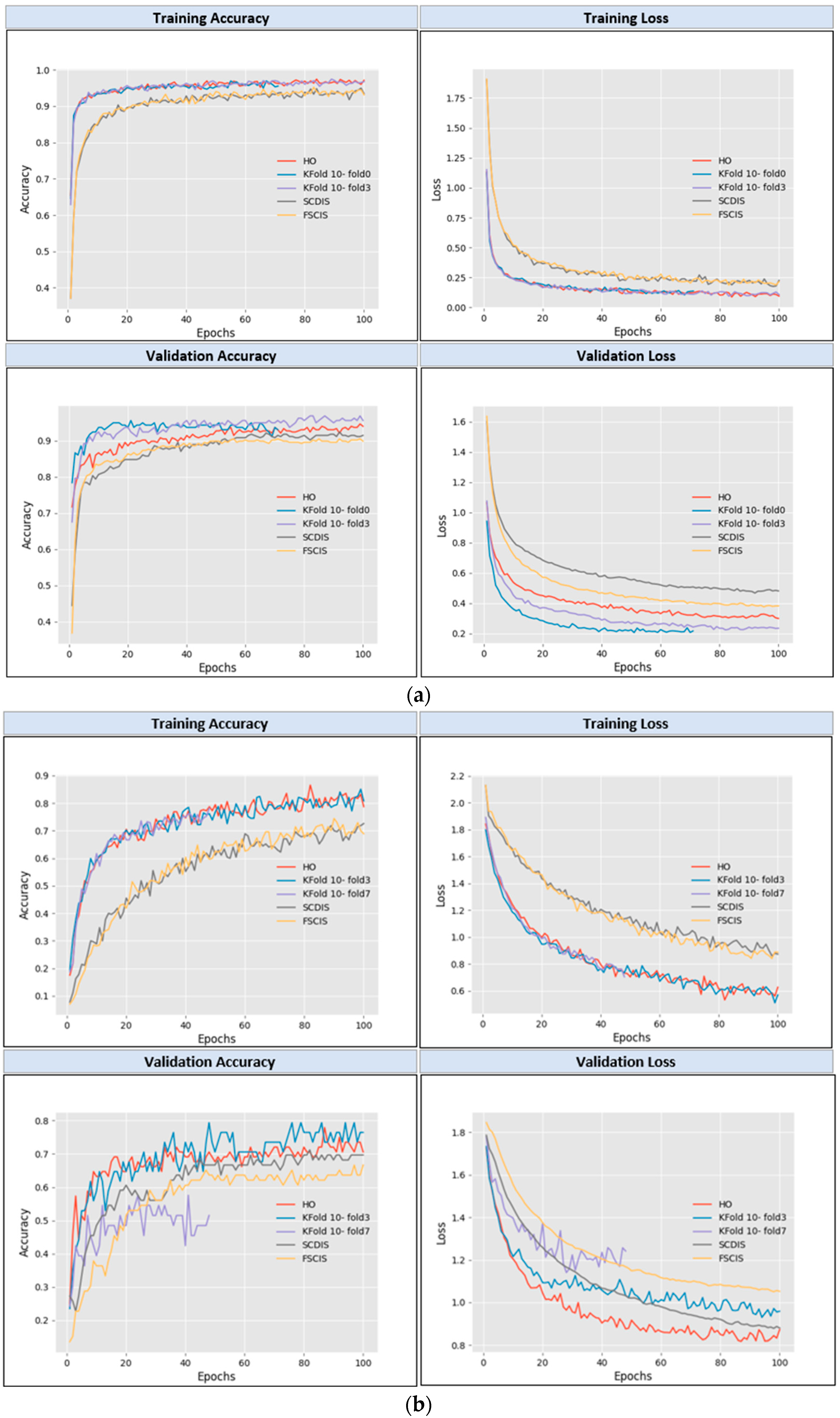
After training the model, the learning curves were analyzed. By observation, their respective training and validation lines seem smoother and more stable for the models trained with datasets split by the FCDIS and FSCIS approaches, compared to the ones built from datasets derived from traditional techniques. Such an aspect can be found in Figure 13, which shows a set of training/validation accuracy-loss plots, regarding a training session of 100 epochs over datasets built from both of the previously presented image collections (bridge defects and grapevine varieties). As observed, some models finished earlier, due to the use of an early stopping control callback—described in the previous section. This implies that the potential of learning was reached before the last epoch for the training sessions. In Figure 13a, the KFCV10-fold0 finished at epoch 71, while in Figure 13b, for the KFCV10-fold7, the final epoch was 48. Such control over training progress is of high relevance—as demonstrated in previous works [1]—to reach models with optimized performance in a timelier manner while simultaneously preventing overfitting.

4.2. Assessment with the Data Reserved for Testing

Based on the previously documented grapevine and bridge defects imagery, datasets compliant with a standard DL training process were built, resorting to both the traditional and proposed approaches. These models were then assessed and compared in terms of accuracy using a $D_{Tst}$ reserved for this purpose (i.e., image subsets isolated from the models’ training, as specified in Figure 4). The respective results for $D_{Tst}^{BDI}$ and $D_{Tst}^{GLI}$ can be consulted in

Table 3. Accuracy results for models trained with $D_{Tst}^{BDI}$.

Dataset Split Approaches		Xception
		Nadam		SGD
		Acc	ESE	Acc	ESE
SCDIS		0.90	100	0.86	100
FSCIS		0.88	100	0.81	100
Hold out		0.89	100	0.82	100
KFCV10	Fold 0	0.89	71	0.86	100
	Fold 1	0.88	100	0.84	100
	Fold 2	0.87	100	0.82	100
	Fold 3	0.90	100	0.81	100
	Fold 4	0.88	100	0.82	100
	Fold 5	0.88	100	0.85	100
	Fold 6	0.89	100	0.83	100
	Fold 7	0.89	100	0.82	100
	Fold 8	0.88	89	0.84	100
	Fold 9	0.88	100	0.83	100
	Mean KFCV10	0.88		0.73

and

Table 4. Accuracy results for models trained with datasets $D_{Tst}^{GLI}$.

Dataset Split Approaches		Xception
		Nadam		SGD
		Acc	ESE	Acc	ESE
SCDIS		0.70	100	0.67	100
FSCIS		0.76	100	0.74	100
Hold out		0.75	100	0.69	100
KFCV10	Fold 0	0.70	100	0.67	100
	Fold 1	0.65	100	0.70	100
	Fold 2	0.70	98	0.68	100
	Fold 3	0.74	100	0.71	100
	Fold 4	0.68	94	0.68	100
	Fold 5	0.68	100	0.65	100
	Fold 6	0.65	92	0.67	100
	Fold 7	0.61	48	0.60	100
	Fold 8	0.65	84	0.67	100
	Fold 9	0.67	100	0.71	100
	Mean KFCV10	0.67		0.67

, respectively.

As illustrated in Table 3 and Table 4, the models employing the proposed techniques completed the training up to epoch 100, while some models using traditional techniques failed to reach that limit, due to the transversal use of an early stopping monitor in the supervision of the training process.

In Table 3, the accuracy results demonstrate that the models trained with SCDIS and FSCIS outperform the HO, as well as 90% of the KFCV10 group. Additionally, Table 4 highlights that the proposed methods performed better than the ones with conventional techniques. These findings underscore their continual outperformance relative to the mean performance achieved by KFCV10. Regarding the optimizers, it is worth noting that the models trained with Nadam outperformed the ones supported by SGD.

4.3. Assessment with External Imagery Sources

An extension to the assessment of the previous models was carried out, using $D_{Ext\_Tst}^{GLI}$ and $D_{Ext\_Tst}^{BDI}$ with a set of classes that seamlessly match the one that characterizes the former datasets applied for training, as previously explained in the materials and methods section. To that end and for the sake of contention while still ensuring some representativeness, 10 random images per class were considered.

The trained models were evaluated against the above-mentioned external data and the results are presented in

Table 5. Accuracy of models using the $D_{Ext\_Tst}^{BDI}$.

Dataset Split Approaches		Xception
		Nadam	SGD
		Acc	Acc
SCDIS		0.75	0.68
FSCIS		0.75	0.72
Hold out		0.72	0.70
KFCV10	Fold 0	0.72	0.73
	Fold 1	0.72	0.77
	Fold 2	0.77	0.70
	Fold 3	0.73	0.73
	Fold 4	0.68	0.75
	Fold 5	0.77	0.67
	Fold 6	0.75	0.75
	Fold 7	0.75	0.70
	Fold 8	0.73	0.70
	Fold 9	0.72	0.68
	Mean KFCV10	0.73	0.72

for $D_{Ext\_Tst}^{BDI}$, and in

Table 6. Accuracy of models using the $D_{Ext\_Tst}^{GLI}$.

Dataset Split Approaches		Xception
		Nadam	SGD
		Acc	Acc
SCDIS		0.32	0.27
FSCIS		0.25	0.22
Hold out		0.22	0.20
KFCV10	Fold 0	0.25	0.25
	Fold 1	0.25	0.22
	Fold 2	0.25	0.28
	Fold 3	0.23	0.28
	Fold 4	0.32	0.28
	Fold 5	0.23	0.27
	Fold 6	0.23	0.23
	Fold 7	0.25	0.25
	Fold 8	0.27	0.23
	Fold 9	0.25	0.30
	Mean KFCV10	0.25	0.26

for $D_{Ext\_Tst}^{GLI}$.

Considering the outcomes presented in Table 5, one can infer that SCDIS- and FSCIS-based Xception/Nadam models clearly outperform HO, and, compared to KFCV10-based models, most of the accuracies are matched or surpassed (8/10). A less noticeable tendency can be observed for the FSCIS-based Xception/SGD model, which was still capable of outperforming both HO and half of the KFCV10-based models. In Table 6, the SCDIS-based model stands out, largely surpassing HO and most of the KFCV10-based models for both Xception/Nadam and Xception/SGD combinations. Less successful was the FSCIS model, which could only prevail over HO and a few KFCV10 models.

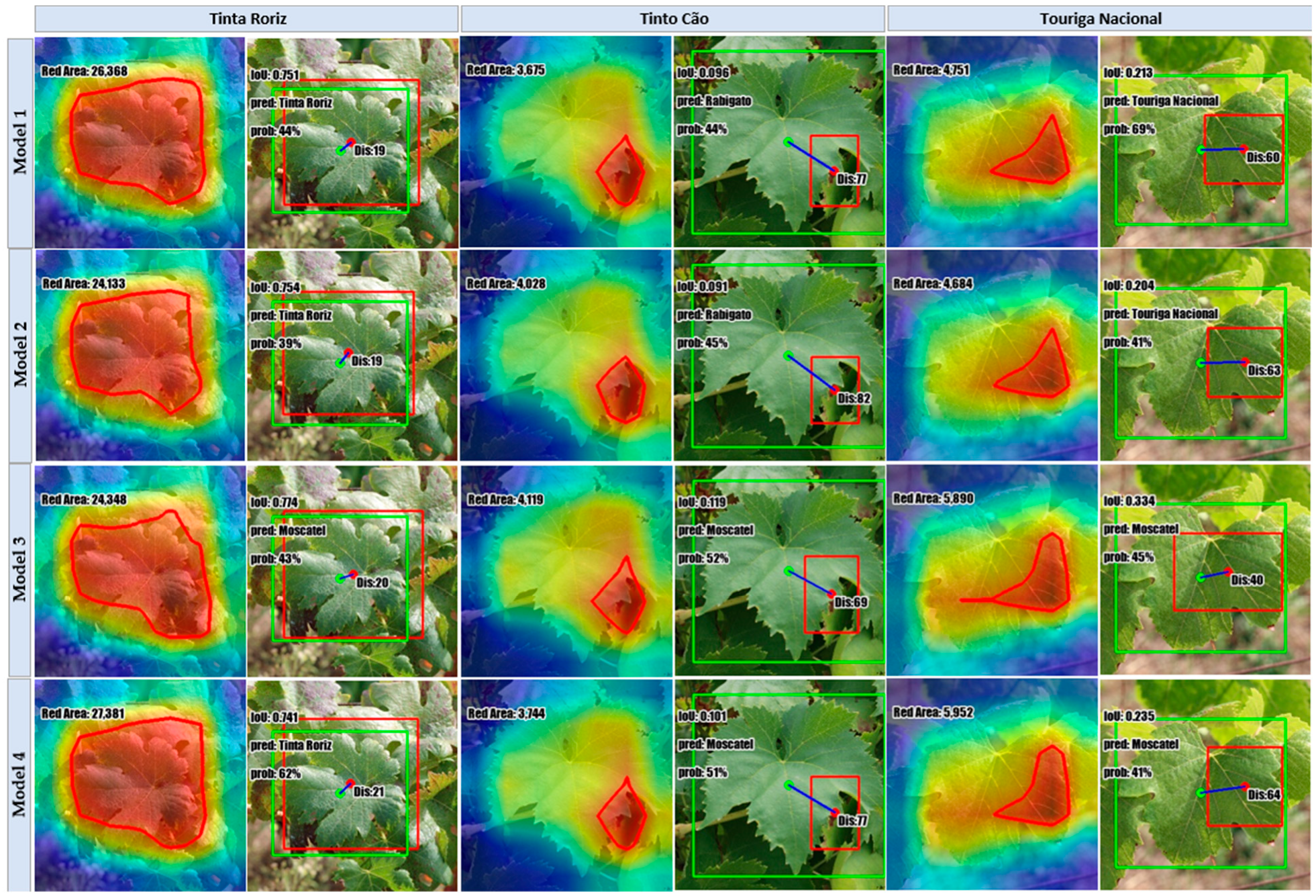
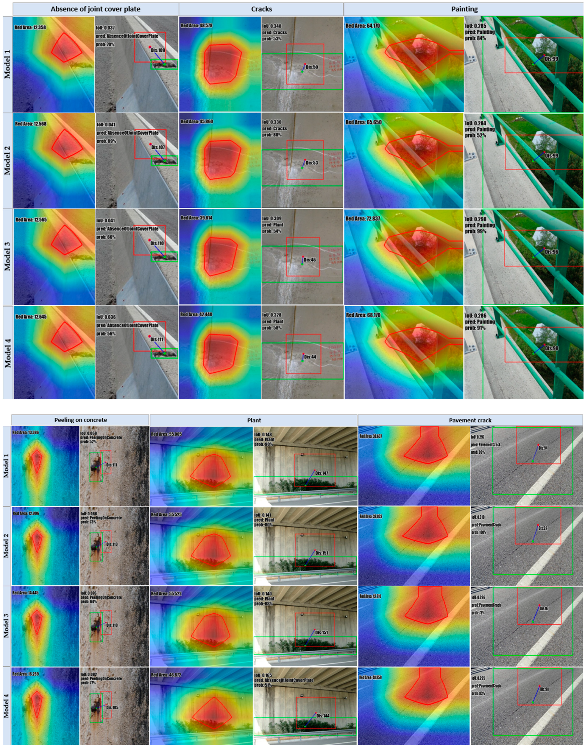
4.4. Attention Mechanisms Assessment with External Imagery Sources

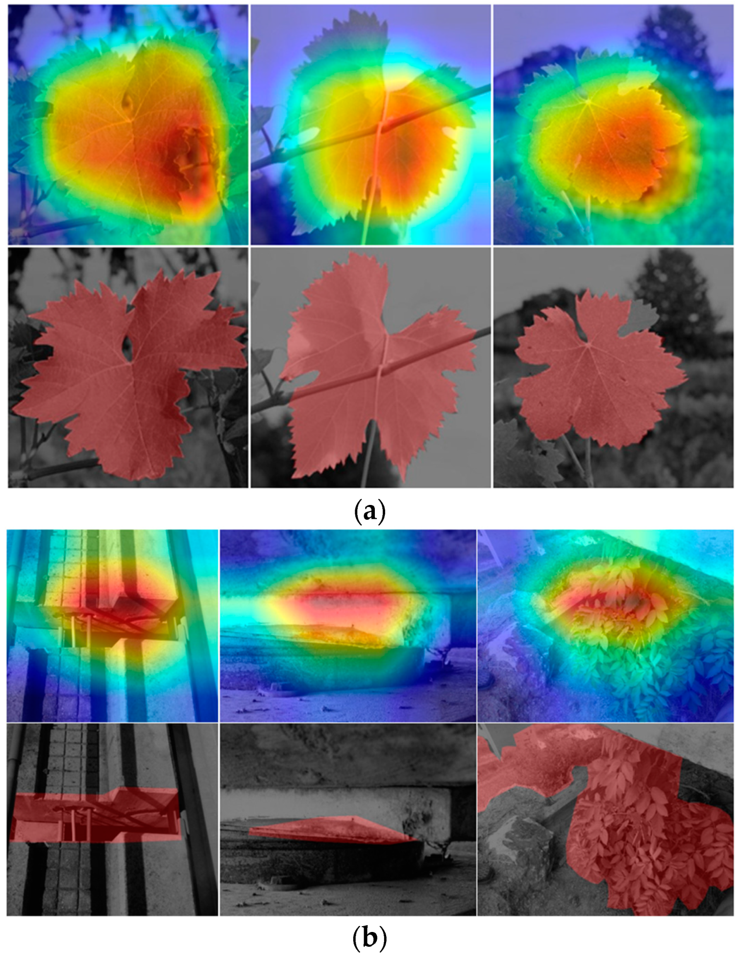
Gradient-weighted class activation mapping (Grad-CAM)-based IoU allows a more comprehensive understanding of the model’s performance, more specifically, by exploring the spatial accuracy and localization precision of the predictions. A more detailed examination of the salient features and attention areas associated with the models can be attained, aligning with eXplainable artificial intelligence (XAI) strategies, which promote enhanced interpretability and may provide directions for improving accuracies.

In this section, the models that reached the highest performances in the previous assessment addressing classification tasks were considered. Before applying them in the proposed analysis, a couple of preliminary steps were carried out: (i) determining the Grad-CAM-generated area and (ii) annotating the corresponding ground truth regions in the images involved in the assessment, i.e., those related to Grad-CAM and the masks associated with the samples (Figure 14). One should note that the biases involved are highly dependent on the Grad-CAM estimations provided by the previously trained models upon $D_{Tr-Val}^{BDI}$, $D_{Tr-Val}^{GLI}$.

As for the computation of Grad-CAM for each image, only the most salient attention area is considered, i.e., the zone of the image highlighted in red. Subsequently, for each image, a bounding box is computed around that salient area, and the distance between the resulting delimitation and the corresponding ground-truth region is calculated, based on the respective centroids. Besides the displacement between the computed centroids (Dis), three other Grad-CAM-based elements were considered as key parameters: classification accuracy (Acc), IoU, and Grad-CAM size (GCS).

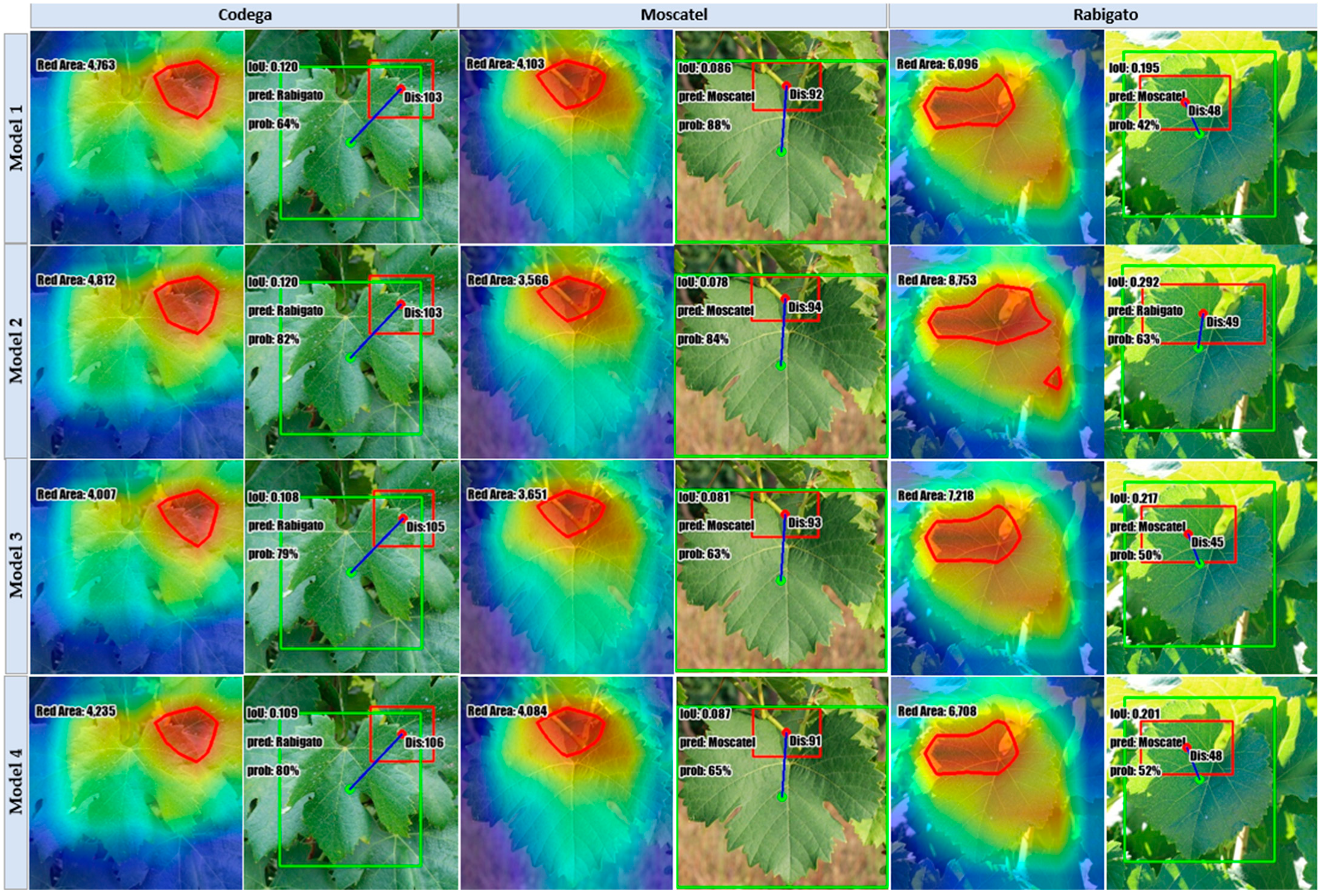
Regarding the analysis made for the $D_{Ext\_Tst}^{GLI}$, Figure 15 showcases the Grad-CAM outcomes for the top Xception models trained with the several considered approaches: FSCIS, FCDIS, HO, and the best classifier that resulted from KCVF10. Each image is accompanied by a short text denoting the respective key parameters formerly specified. Following a similar organization and structure, Figure 16 depicts the results in the context of the $D_{Ext\_Tst}^{BDI}$.

Instead of closely examining the parameters for each specific image, the focus was on calculating the mean values of key parameters for each class within both datasets, aiming to provide an overview of the models’ performances at a more generalized level across different classes.

Table 7. Prediction results upon the $D_{Ext\_Tst}^{GLI}$ for Xception Nadam.

Class	SCDIS				FSCIS				HO				KFCV10—Fold3
	µAcc	µIoU	µGCS	µDis	µAcc	µIoU	µGCS	µDis	µAcc	µIoU	µGCS	µDis	µAcc	µIoU	µGCS	µDis
Codega	0.00	0.12	4393	85	0.00	0.13	4880	82	0.00	0.10	3541	87	0.00	0.11	4139	86
Moscatel	0.90	0.173	7349	69	0.50	0.16	6311	72	0.70	0.14	5396	75	0.00	0.15	4996	70
Rabigato	0.60	0.19	7678	67	0.80	0.19	7478	70	0.50	0.15	6099	76	0.70	0.15	6000	72
Tinta Roriz	0.20	0.24	8231	63	0.10	0.23	7731	62	0.10	0.24	7956	62	0.00	0.24	8526	62
Tinto Cao	0.00	0.21	7961	58	0.00	0.23	8911	58	0.00	0.16	6467	62	0.10	0.15	6415	65
Touriga Nacional	0.20	0.23	7707	67	0.10	0.21	7652	70	0.00	0.28	8784	63	0.00	0.22	7915	70
Total mean	0.38	0.19	7220	68	0.25	0.19	7160	69	0.22	0.18	6374	71	0.13	0.17	6332	71

and

Table 8. Prediction results for the proposed dataset splits for the Xception model using Nadam optimizer upon $D_{Ext\_Tst}^{BDI}$. AJCP—absence of joint cover plate; PC—pavement crack; PoC—peeling on concrete.

Class	SCDIS				FSCIS				HO				KFCV10—Fold3
	µAcc	µIoU	µGCS	µDis	µAcc	µIoU	µGCS	µDis	µAcc	µIoU	µGCS	µDis	µAcc	µIoU	µGCS	µDis
AJCP	0.90	0.18	42,969	139	0.90	0.20	48,068	137	0.80	0.19	46,502	140	0.80	0.18	45,516	141
Cracks	0.70	0.21	39,203	126	0.70	0.21	38,771	129	0.40	0.18	38,429	132	0.60	0.20	37,225	127
Painting	0.50	0.20	36,071	124	0.50	0.18	32,077	117	0.90	0.20	33,226	107	0.70	0.21	36,871	118
PC	0.90	0.16	27,457	149	0.90	0.16	26,962	148	0.90	0.15	28,107	147	1.00	0.15	28,070	147
PoC	0.50	0.17	30,665	125	0.50	0.17	30,473	126	0.50	0.17	31,801	125	0.50	0.18	31,065	124
Plant	1.00	0.17	49,259	144	1.00	0.16	48,878	146	0.50	0.16	48,549	145	0.80	0.17	49,576	145
Total mean	0.75	0.18	37,604	135	0.75	0.18	37,538	134	0.67	0.18	37,769	133	0.73	0.18	38,054	134

indicate the numeric results associated with the mean values of key parameters corresponding to Xception/Nadam pairs.

Table 7 presents the outcomes obtained regarding the $D_{Ext\_Tst}^{GLI}$, wherein both SCDIS and FSCIS outperform the opponents. In particular, the SCDIS split method was the best in this series, yielding an accuracy of 38%, an µIoU = 0.19, a µGCS = 7220, and a µDis = 68.

Additionally, Table 8 presents the results for the $D_{Ext\_Tst}^{BDI}$, relying on the same metrics. Once again, the most effective models originated from both of the proposed dataset splitting methods. Notably, these models attained similar performances: µIoU = 0.18, µAcc = 75%, µGCS = 37,604, and µDis = 135 for FSCIS; and µIoU = 0.18, µAcc = 75%, µGCS = 37,538, and µDis = 134 for SCDIS.

On the other hand, the results show a spotlight pattern—greater IoU scores align with higher classification accuracies, particularly when the region of attention is closer to the ground-truth center. This pattern underscores the relationship between precise localization and the model’s effectiveness in correctly classifying objects. These observations across the tables emphasize the significance of spatial awareness in improving the overall accuracy of the classification process.

5. Discussion, Summary, and Conclusions

In this section, the main findings and contributions of this work are summarized. This research work hypothesizes feature-aware data splitting as a strategy to enhance the performance of classification models in a timelier manner, at the expense of traditional techniques, such as KFCV and HO. Therefore, datasets of two distinct contexts were considered for the sake of condition variability: one related to bridge defects and the other associated with grapevine leaves, for phenotyping distinction.

Regarding the proposed splitting approaches, the first one employs a feature-oriented clustering-based splitting technique, with a selection method based on the centroid distance of each cluster to the global centroid—FCDIS. The second approach revolves around sorting and picking images at the feature space level, based on their distance to the global centroid—FSCIS. The main goal is to compare both of these methods with conventional techniques, namely, HO and KFCV with 10 folds.

For training the classification models, the Xception architecture was utilized with a learning rate of 10⁻³, and optimizers including Nadam and SGD, and the maximum number of training epochs was set to 100. In most of the experiments, the proposed FCDIS and FSCIS methods outperformed the traditional approaches. Furthermore, the accuracy-loss plots illustrated a more stable training process with the proposed methods, characterized by an apparent reduction in abrupt fluctuations associated with these metrics across training sessions.

To assess the trained classifiers, external datasets were considered for a Grad-CAM-based evaluation, while IoU was used as another metric for performance comparison. The results pointed out that the models trained with the proposed methods had a consistently higher capacity in identifying the relevant areas of the images, highlighting them as more effective compared to the ones trained with traditional splitting techniques.

In comparison to the existing approaches, particularly those employing traditional dataset splitting techniques, such as HO, resampling, normal, repeated, nested, and leave-one-out KFCV, the proposed methods of this work—FCDIS and FSCIS—confirm and consolidate the importance of using strategic division for the attainment of more accurate models, with decreased computational burdens, while mitigating the need of multi-step procedures (e.g., KFCV), at least when relatively short volumes of classes and examples are involved.

It is noteworthy that a clustering-based method has been addressed in, at least, one of the aforementioned works found in the literature. However, a K-fold-based strategy was still applied to select data within clusters [37]. In contrast, the proposed FCDIS and FSCIS methods provide strong evidence that one-shot data organization is a possible avenue to attain models of top accuracy, as the experimental results demonstrate. Therefore, this study also intends to inspire and challenge the scientific community and DL practitioners to include strategic dataset splitting methods, either based on the proposed ones or supported in brand-new approaches, to save time and computational resources, while aiming to develop inference models that can operate near their full potential.

Notwithstanding, as the used datasets are relatively short, and the hardware and software setup are more oriented to DL prototyping, further tests are encouraged, involving wider data classes and examples, and resorting to high-performance computing. Moreover, the generalizability of the proposed splitting techniques beyond the addressed datasets and inference tasks requires deeper investigation through, namely, the inclusion of complementary key-factors—for example, considering uncertainty and context-sensitive false/true positives risk assessment—that contribute to explaining the models’ behavior and, therefore, broadly optimize the training processes.