
A Systematic Evaluation of Recurrent Neural Network Models for Edge Intelligence and Human Activity Recognition Applications

 , , and
Abstract
1. Introduction
1.1. Motivation and Challenges
1.2. Contributions and Key Features
- We present a comprehensive application of device mapping research workflow that can be commonly adapted for optimizing RNN models onto a resource-constrained edge (see Section 3). This will help with reducing the research time required for methodical workflows in this context.
- We focused on the HAR-based EI-RNN evaluation and optimization of five different RNN units sandboxed apart from the classic LSTM structures (see Section 2.1, Section 2.2, Section 2.3, Section 2.4, Section 2.5 and Section 2.6).
- We used eight different HAR datasets (see Table 3 and Table 4, Section 4.2.9 for important details) and two evaluation methods, namely, the hold-out method and cross-validation method.
- We conducted an in-depth performance analysis of both training and compression techniques applied to RNNs (see Section 5.1 and Section 5.2). To the best of our knowledge, the exact details of both these critical aspects have rarely been presented with clarity from an implementation point of view.
- The key takeaways based on this empirical evaluation study will be important for practitioners and researchers in this problem domain.
2. Background and Related Work
2.1. Vanilla RNN
2.2. LSTM RNN
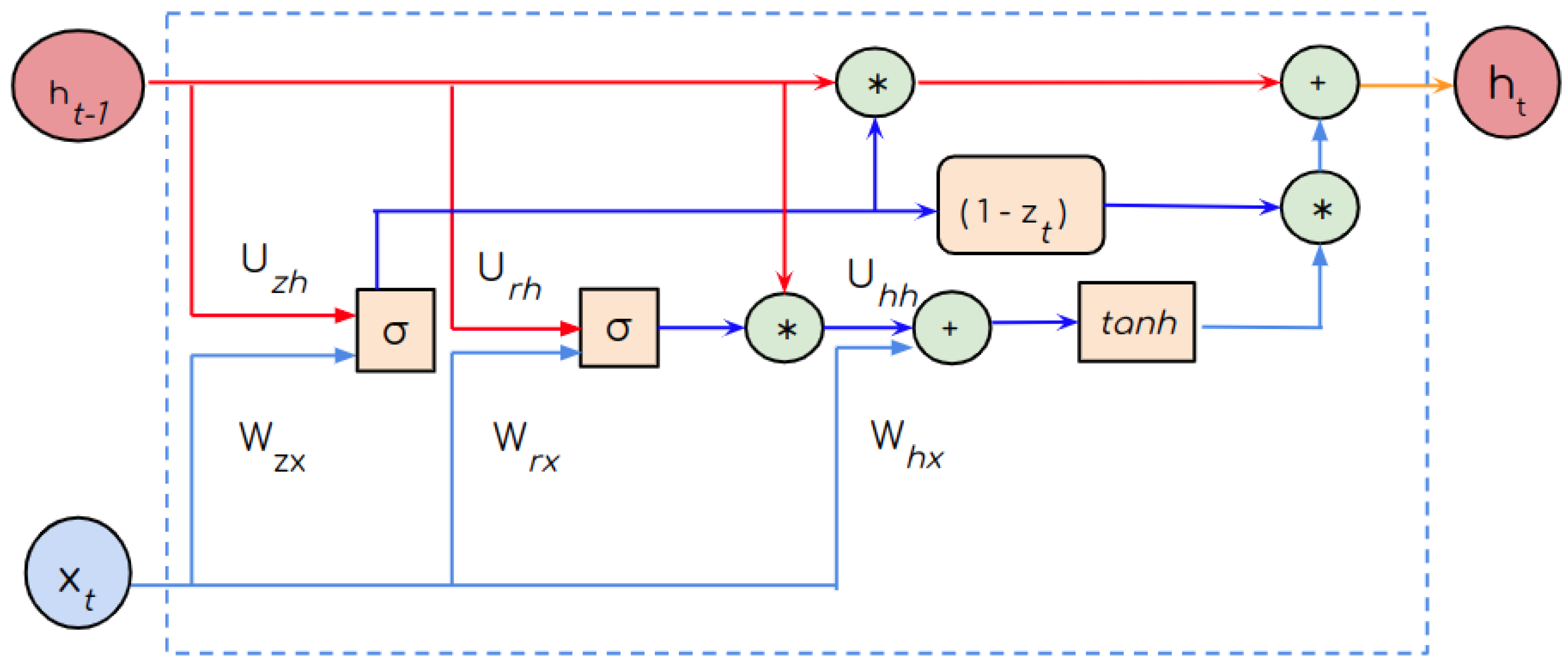
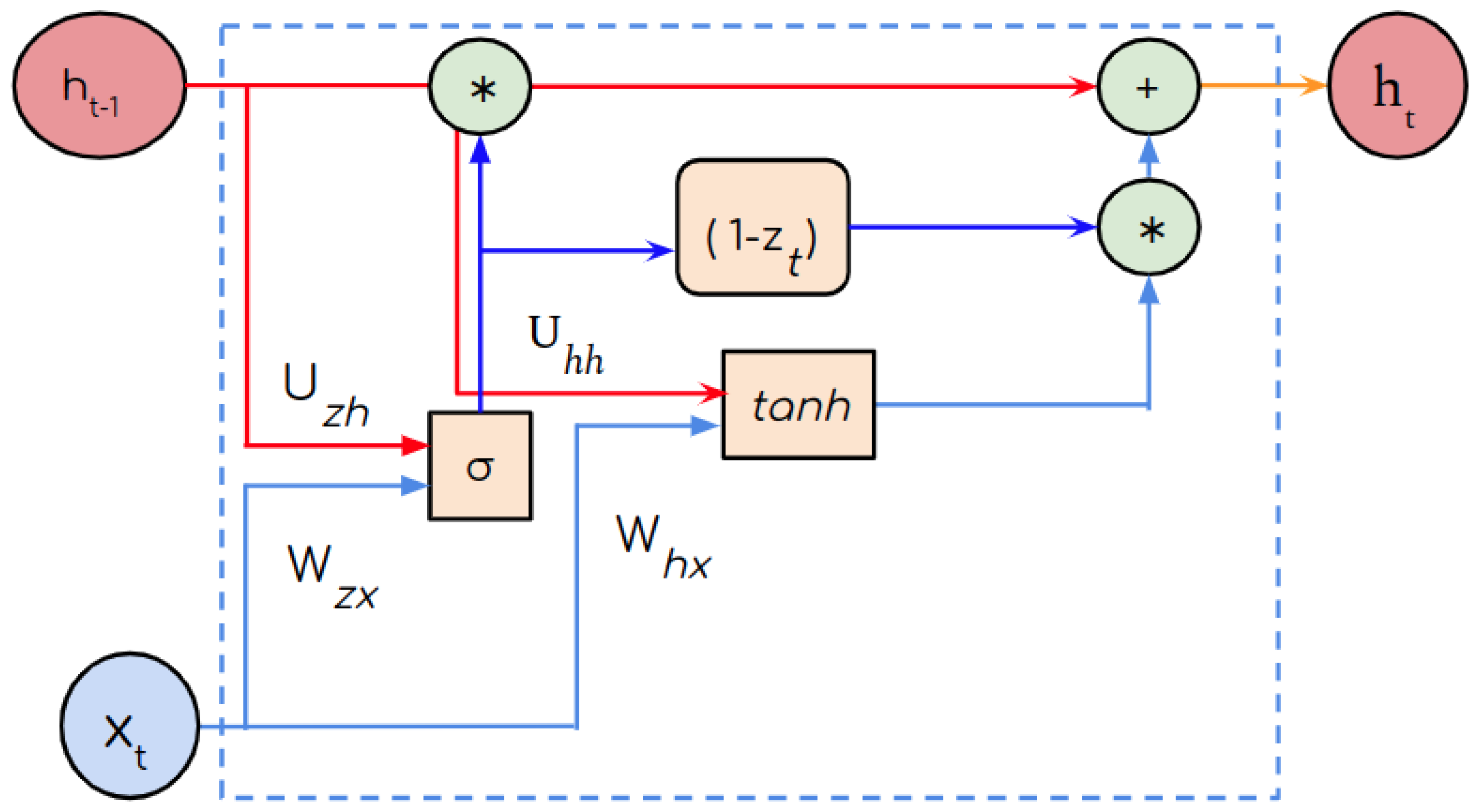
2.3. GRU
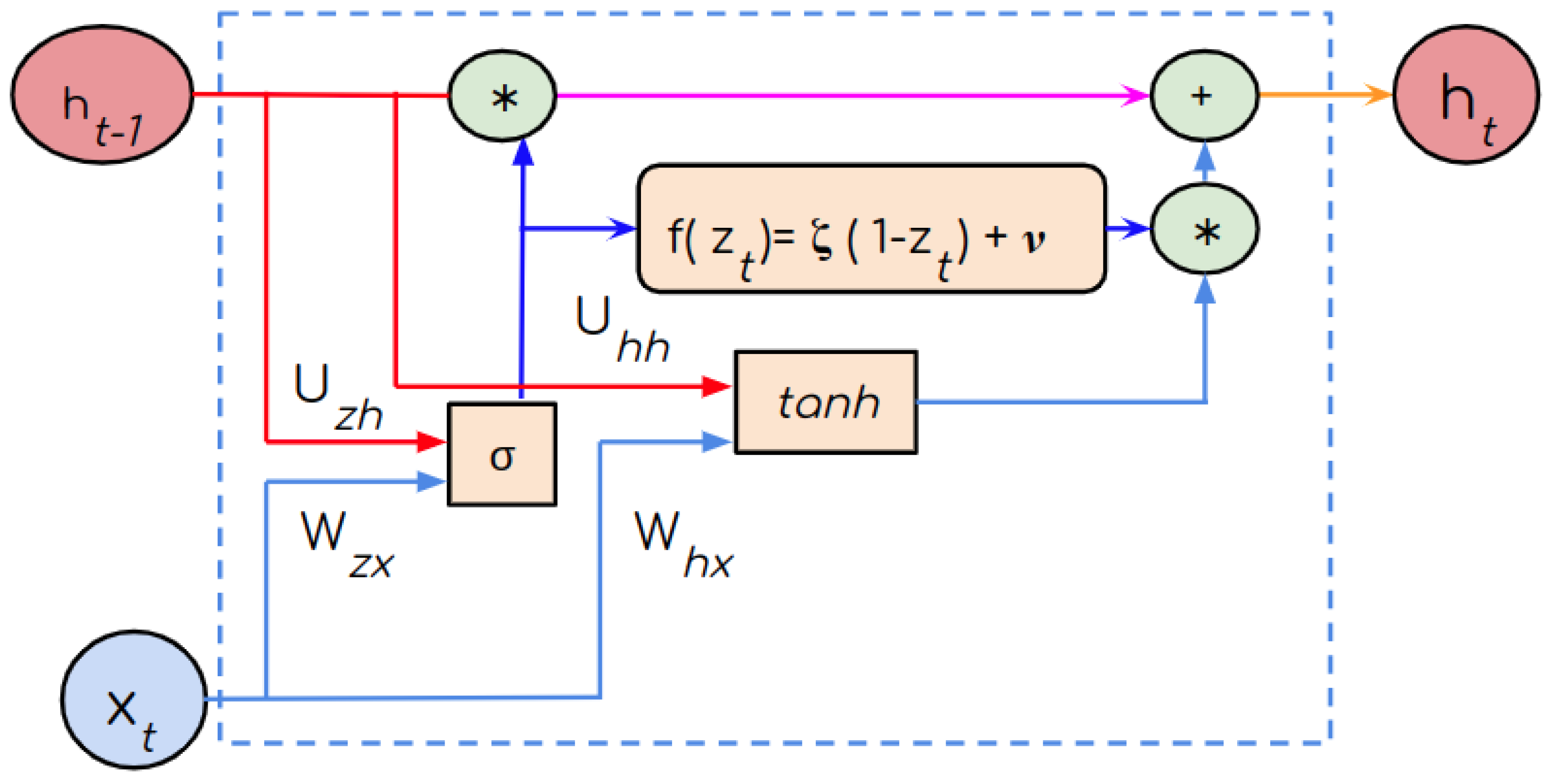
2.4. FGRNN
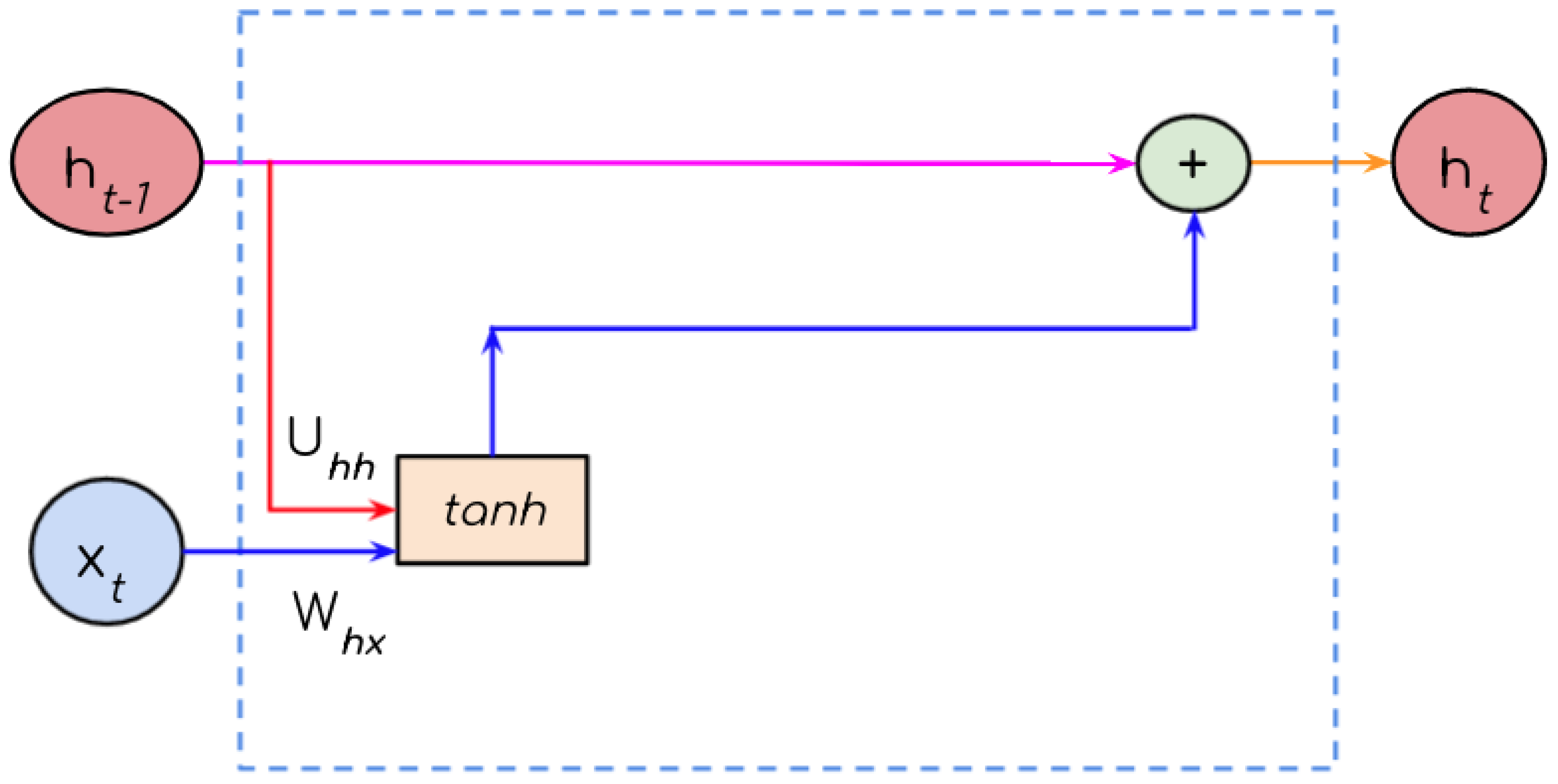
2.5. FRNN
2.6. UGRNN
3. Research Workflow
4. Experiments
4.1. Experimental Settings
4.2. Application and Datasets

| SI No. | Dataset | Input Sensor | Train Samples | Val Samples | Test Samples | Time Steps | Input Features | Output Labels | Freq. (Hz) |
|---|---|---|---|---|---|---|---|---|---|
| 1 | DSA [49] (B) | A, M | 6976 | 1232 | 912 | 125 | 5625 | 19 | 25 |
| 2 | SPHAR [50] (B) | A, G | 7878 | 1391 | 1030 | 128 | 1152 | 6 | 50 |
| 3 | Opportunity [51] (N) | A, G, M | 54,246 | 9894 | 2684 | 24 | 1896 | 18 | 30 |
| 4 | Pamap2 [52] (B) | A, G, M | 39,452 | 7566 | 6946 | 24 | 1248 | 12 | 100 |
| SI No. | Dataset | Input Sensor | No. of Samples (SNOW) | No. of Samples (FNOW) | No. of Classes | Sampling Frequency (Hz) | No. of Features | Balanced |
|---|---|---|---|---|---|---|---|---|
| 1 | MHEALTH [53] | A, G, M | 2555 | 1335 | 12 | 50 | 5750 | True |
| 2 | USCHAD [54] | A, G | 9824 | 5038 | 12 | 100 | 3000 | False |
| 3 | WHARF [55] | A | 3880 | 2146 | 12 | 32 | 480 | False |
| 4 | WISDM [56] | A | 20,846 | 10,516 | 6 | 20 | 300 | False |
4.2.1. Daily and Sports Activities Dataset
4.2.2. Smart Phone Human Activity Recognition Dataset
4.2.3. Opportunity Dataset
4.2.4. Physical Activity Monitoring for Aging People Dataset
4.2.5. Mobile Health Dataset
4.2.6. University of Southern California Human Activity Dataset
4.2.7. Wearable Human Activity Recognition Folder Dataset
4.2.8. Wireless Sensor Data Mining Dataset
4.2.9. Finer Details of the Datasets
4.3. Evaluation Protocols and Metrics
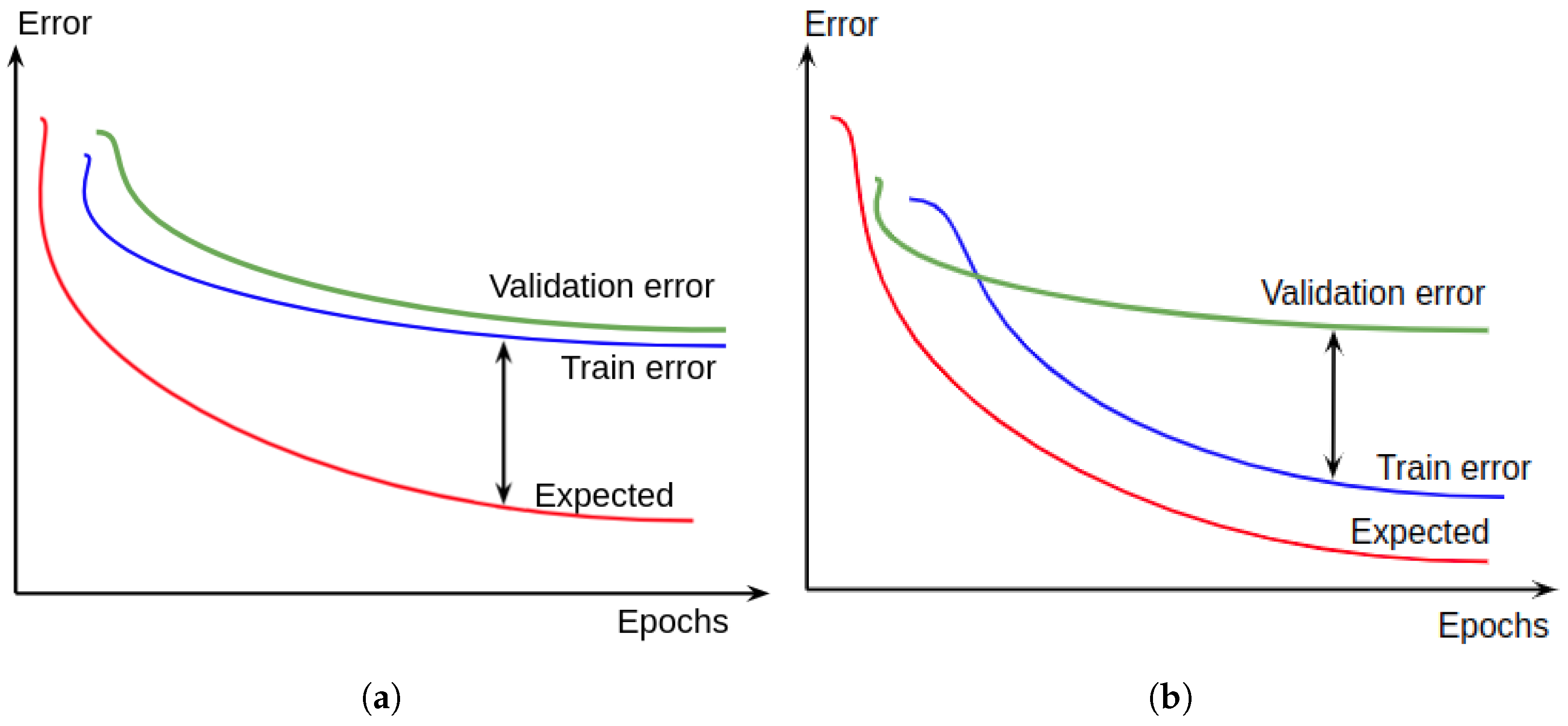
- Holdout method: In this method, datasets are split into three sets, i.e, training set, validation/holdout set, and testing set. Here, the training set is the subset of data used to learn the temporal pattern in the time-series data. The error associated with this is called training error. Validation or hold-out set is the subset of data used to guide the selection of hyperparameters. The error associated with this is called validation error. The test set is the subset of data used to measure the model’s performance on a new unseen sample. The error associated with this is called testi error. The split ratio affects the model’s performance.
- Cross-validation method: In this method, datasets are split into k nonoverlapping subsets. In each trial, one of them is chosen as a test set and the rest is used as the training set. Test error is estimated by taking the average test error across k trials.
- Accuracy: This metric denotes the total number of correct predictions of classes against their actual labels.
- F1 score: This metric is the weighted average of precision and recall. Precision is the ratio of correctly classified positive observations to the total classified positive observations. Recall is the ratio of correctly classified positive observations to all observations in actual class.
5. EI-RNN Optimization and Analysis
- EI-RNN training on host/cloud GPU;
- EI-RNN compression on host/cloud GPU;
- EI-RNN inference on the edge (RPi).
5.1. EI-RNN Training
5.1.1. Initial Settings
5.1.2. Train–Debug Cycle
5.1.3. Hyperparameter Tuning and Generalization
5.2. EI-RNN Compression
5.3. EI-RNN Inference
6. Results and Discussion
6.1. Performance Evaluation Using Hold-Out Method of Training and Subsequent Compression
6.2. Performance Evaluation Using K-Fold Cross-Validation Training and Subsequent Compression
6.3. Inference Evaluation on Raspberry Pi
- Apart from LSTM, the other RNNS like fast gates like FastGRNN, FastRNN, UGRNN, and GRU are potential candidates for application in device-mapping edge-based RNN modeling studies. Similar studies were conducted in Ref. [28]. The Table 17 from Ref. [28] shows the performance of the RNNs but with different hyperparameters used for the RNN architecture.
- LSTM and GRU require significantly longer training and inference time compared to the other RNN units that we studied.
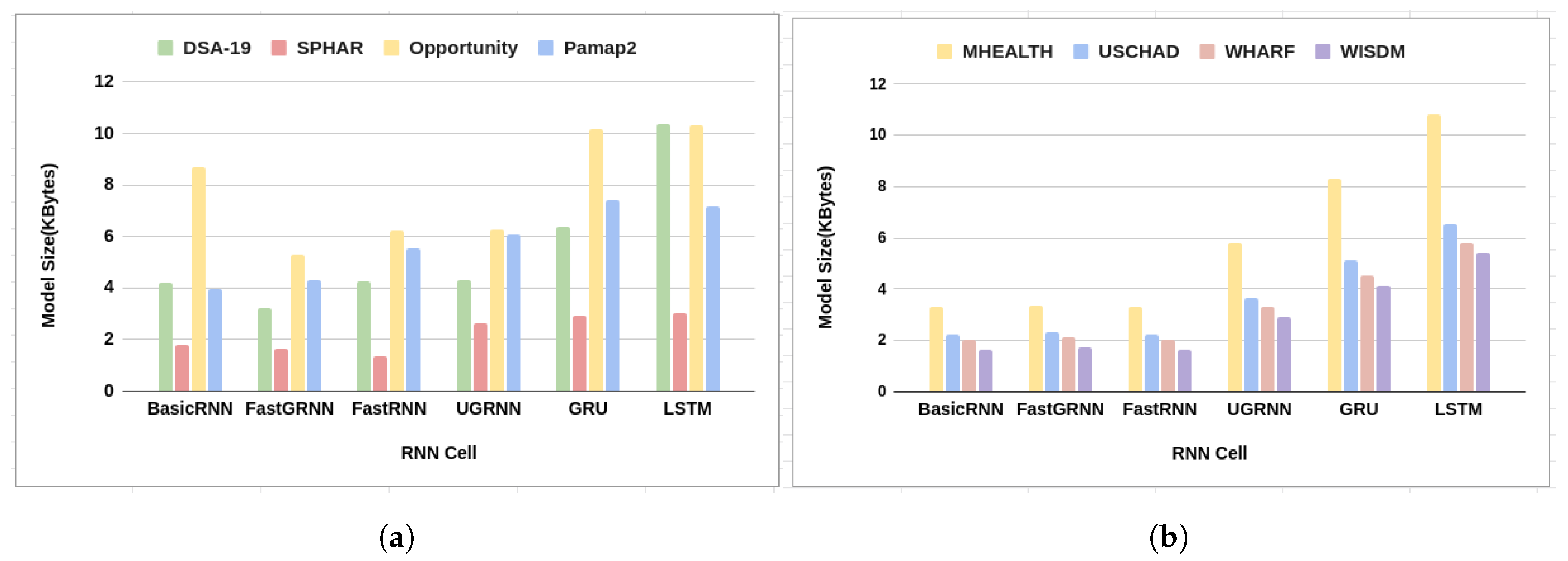
- LSTM and GRU are bulkier on the edge device than FastRNN, FastGatedRNN, and UGRNN.
- Fast gates like FastGRNN and FastRNN are memory-efficient for edge devices, but they show performance deviation compared to the other RNNs of around 0 to 19% across all considered datasets.
- UGRNN are also potential candidates for edge-based RNN model mapping, showing good performance and smaller memory sizes compared to LSTM and GRU.
- Data collection and preprocessing play important roles in training the RNNs and consume significant time.
- If the class distribution of the dataset is unbalanced, we saw a drop in the F1 score of the RNN model.
- A hidden state size of 16 and a single layer are optimal for edge mapping for HAR applications. Increasing the hidden size or layer size improves performance but adversely affects the model size.
- Regularization methods like dropout improve model performance after any degradation due to the compression applied on the dense RNN models.
- A combination of compression techniques is better than singleton methods.
- For Low-Rank Parameterization, the decomposition rank affects the model size and performance of RNNs. Higher ranks improve performance but increase the model size proportionally.
- The inference time on a Raspberry Pi was directly dependent on the time steps, the input feature size the RNN was processing, and the complexity of the RNN cell and architecture.
- The complex workflows for application to device mapping have forced developers to be inventive. Dealing with frameworks and third-party packages and libraries is complex.
7. Conclusions and Future Scope
Author Contributions
Funding
Data Availability Statement
Acknowledgments
Conflicts of Interest
Abbreviations
| RNN | Recurrent Neural Network |
| HAR | Human Activity Recognition |
| GPU | Graphics Processing Unit |
| EI-RNN | Edge-Intelligent RNN |
| IoT | Internet of Things |
| LSTM | Long Short-Term Memory |
| GRU | Gated Recurrent Unit |
| FRNN | Fast Recurrent Neural Network |
| FGRNN | Fast Gated Recurrent Neural Network |
| UGRNN | Unitary Gated Recurrent Neural Network |
| RPi | Raspberry Pi |
| DL | Deep Learning |
| AI | Artificial Intelligence |
| CNN | Convolutional Neural Network |
| MCU | Microcontroller Unit |
| ELL | Embedded Learning Library |
| SoC | System on Chip |
| LMF | Low-Rank Matrix Factorization |
| SVD | Singular Value Decomposition |
| DSA | Daily and Sports Activities |
| SPHAR | Smart Phone Human Activity Recognition |
| Oppo | Opportunity |
| PAMAP | Physical Activity Monitoring for Aging People |
| MHEALTH | Mobile HEALTH |
| USC-HAD | University of Southern California Human Activity Dataset |
| WHARF | Wearable Human Activity Recognition Folder |
| WISDM | Wireless Sensor Data Mining |
| NaN | Not a Number |
| API | Application Programming Interface |
| wandb | Weights and Biases Tool |
| RMS Prop | Root Mean Squared Propagation |
Appendix A
References
- Kolen, J.; Kremer, S. Gradient flow in recurrent nets: The difficulty of learning longterm dependencies. In A Field Guide to Dynamical Recurrent Network; IEEE: Piscataway, NJ, USA, 2010. [Google Scholar]
- Martens, J.; Sutskever, I. Learning recurrent neural networks with hessian-free optimization. In Proceedings of the 28th International Conference on Machine Learning, Washington, DC, USA, 28 June–2 July 2011. [Google Scholar]
- Collins, J.; Sohl-Dickstein, J.; Sussillo, D. Capacity and trainability in recurrent neural networks. arXiv 2016, arXiv:1611.09913. [Google Scholar]
- Lalapura, V.S.; Amudha, J.; Satheesh, H.S. Recurrent neural networks for edge intelligence: A survey. ACM Comput. Surv. 2021, 54, 1–38. [Google Scholar] [CrossRef]
- Amudha, J.; Thakur, M.S.; Shrivastava, A.; Gupta, S.; Gupta, D.; Sharma, K. Wild OCR: Deep Learning Architecture for Text Recognition in Images. In Proceedings of the International Conference on Computing and Communication Networks, Manchester, UK, 19–20 November 2022; Springer: Berlin/Heidelberg, Germany, 2022; pp. 499–506. [Google Scholar]
- Vanishree, K.; George, A.; Gunisetty, S.; Subramanian, S.; Kashyap, S.; Purnaprajna, M. CoIn: Accelerated CNN Co-Inference through data partitioning on heterogeneous devices. In Proceedings of the 2020 6th International Conference on Advanced Computing and Communication Systems (ICACCS), Coimbatore, India, 6–7 March 2020; IEEE: Piscataway, NJ, USA, 2020; pp. 90–95. [Google Scholar]
- Sujadevi, V.G.; Soman, K.P. Towards identifying most important leads for ECG classification. A Data driven approach employing Deep Learning. Procedia Comput. Sci. 2020, 171, 602–608. [Google Scholar] [CrossRef]
- Madsen, A. Visualizing memorization in RNNs. Distill 2019, 4, e16. [Google Scholar] [CrossRef]
- Bengio, Y.; Simard, P.; Frasconi, P. Learning long-term dependencies with gradient descent is difficult. IEEE Trans. Neural Netw. 1994, 5, 157–166. [Google Scholar] [CrossRef] [PubMed]
- Asmitha, U.; Roshan Tushar, S.; Sowmya, V.; Soman, K.P. Ensemble Deep Learning Models for Vehicle Classification in Motorized Traffic Analysis. In Proceedings of the International Conference on Innovative Computing and Communications, Delhi, India, 17–18 February 2023; Gupta, D., Khanna, A., Bhattacharyya, S., Hassanien, A.E., Anand, S., Jaiswal, A., Eds.; Spinger: Singapore, 2023; pp. 185–192. [Google Scholar]
- Ramakrishnan, R.; Vadakedath, A.; Bhaskar, A.; Sachin Kumar, S.; Soman, K.P. Data-Driven Volatile Cryptocurrency Price Forecasting via Variational Mode Decomposition and BiLSTM. In Proceedings of the International Conference on Innovative Computing and Communications, Delhi, India, 17–18 February 2023; Gupta, D., Khanna, A., Bhattacharyya, S., Hassanien, A.E., Anand, S., Jaiswal, A., Eds.; Spinger: Singapore, 2023; pp. 651–663. [Google Scholar]
- Pascanu, R.; Mikolov, T.; Bengio, Y. On the difficulty of training recurrent neural networks. In Proceedings of the International Conference on Machine Learning, PMLR, Atlanta, GA, USA, 17–19 June 2013; pp. 1310–1318. [Google Scholar]
- Lin, J. Efficient Algorithms and Systems for Tiny Deep Learning. Ph.D. Thesis, Massachusetts Institute of Technology, Cambridge, MA, USA, 2021. [Google Scholar]
- Han, S.; Kang, J.; Mao, H.; Hu, Y.; Li, X.; Li, Y.; Xie, D.; Luo, H.; Yao, S.; Wang, Y.; et al. Ese: Efficient speech recognition engine with sparse lstm on fpga. In Proceedings of the 2017 ACM/SIGDA International Symposium on Field-Programmable Gate Arrays, Monterey, CA, USA, 22–24 February 2017; pp. 75–84. [Google Scholar]
- Hochreiter, S.; Schmidhuber, J. Long short-term memory. Neural Comput. 1997, 9, 1735–1780. [Google Scholar] [CrossRef] [PubMed]
- Graves, A. Generating sequences with recurrent neural networks. arXiv 2013, arXiv:1308.0850. [Google Scholar]
- Chung, J.; Gulcehre, C.; Cho, K.; Bengio, Y. Empirical evaluation of gated recurrent neural networks on sequence modeling. arXiv 2014, arXiv:1412.3555. [Google Scholar]
- Cho, K.; Van Merriënboer, B.; Bahdanau, D.; Bengio, Y. On the properties of neural machine translation: Encoder-decoder approaches. arXiv 2014, arXiv:1409.1259. [Google Scholar]
- Cho, K.; Van Merriënboer, B.; Gulcehre, C.; Bahdanau, D.; Bougares, F.; Schwenk, H.; Bengio, Y. Learning phrase representations using RNN encoder-decoder for statistical machine translation. arXiv 2014, arXiv:1406.1078. [Google Scholar]
- Arjovsky, M.; Shah, A.; Bengio, Y. Unitary evolution recurrent neural networks. In Proceedings of the International Conference on Machine Learning, PMLR, New York, NY, USA, 20–22 June 2016; pp. 1120–1128. [Google Scholar]
- David, R.; Duke, J.; Jain, A.; Janapa Reddi, V.; Jeffries, N.; Li, J.; Kreeger, N.; Nappier, I.; Natraj, M.; Wang, T.; et al. TensorFlow lite micro: Embedded machine learning for tinyml systems. Proc. Mach. Learn. Syst. 2021, 3, 800–811. [Google Scholar]
- Microsoft-v2019; ELL: Embedded Learning Library; Microsoft Corporation: Redmond, WA, USA, 2018.
- Banbury, C.; Zhou, C.; Fedorov, I.; Matas, R.; Thakker, U.; Gope, D.; Janapa Reddi, V.; Mattina, M.; Whatmough, P. Micronets: Neural network architectures for deploying tinyml applications on commodity microcontrollers. Proc. Mach. Learn. Syst. 2021, 3, 517–532. [Google Scholar]
- Gu, F.; Chung, M.H.; Chignell, M.; Valaee, S.; Zhou, B.; Liu, X. A survey on deep learning for human activity recognition. ACM Comput. Surv. 2021, 54, 1–34. [Google Scholar] [CrossRef]
- Jordao, A.; Nazare, A.C., Jr.; Sena, J.; Schwartz, W.R. Human activity recognition based on wearable sensor data: A standardization of the state-of-the-art. arXiv 2018, arXiv:1806.05226. [Google Scholar]
- Demrozi, F.; Turetta, C.; Pravadelli, G. B-HAR: An open-source baseline framework for in depth study of human activity recognition datasets and workflows. arXiv 2021, arXiv:2101.10870. [Google Scholar]
- Olah, C. Understanding LSTM Networks. 2015. Available online: http://colah.github.io/posts/2015-08-Understanding-LSTMs/ (accessed on 22 May 2022).
- Kusupati, A.; Singh, M.; Bhatia, K.; Kumar, A.; Jain, P.; Varma, M. Fastgrnn: A fast, accurate, stable and tiny kilobyte sized gated recurrent neural network. In Advances in Neural Information Processing Systems; MIT Press: Cambridge, MA, USA, 2018; Volume 31. [Google Scholar]
- Han, S.; Mao, H.; Dally, W.J. Deep compression: Compressing deep neural networks with pruning, trained quantization and huffman coding. arXiv 2015, arXiv:1510.00149. [Google Scholar]
- Castellano, G.; Fanelli, A.M.; Pelillo, M. An iterative pruning algorithm for feedforward neural networks. IEEE Trans. Neural Netw. 1997, 8, 519–531. [Google Scholar] [CrossRef] [PubMed]
- Reed, R. Pruning algorithms-a survey. IEEE Trans. Neural Netw. 1993, 4, 740–747. [Google Scholar] [CrossRef] [PubMed]
- Guo, Y.; Yao, A.; Chen, Y. Dynamic network surgery for efficient dnns. In Advances in Neural Information Processing Systems; MIT Press: Cambridge, MA, USA, 2016; Volume 29. [Google Scholar]
- Gao, C.; Neil, D.; Ceolini, E.; Liu, S.C.; Delbruck, T. DeltaRNN: A power-efficient recurrent neural network accelerator. In Proceedings of the 2018 ACM/SIGDA International Symposium on Field-Programmable Gate Arrays, Monterey, CA, USA, 25–27 February 2018; pp. 21–30. [Google Scholar]
- Yao, S.; Zhao, Y.; Zhang, A.; Su, L.; Abdelzaher, T. Deepiot: Compressing deep neural network structures for sensing systems with a compressor-critic framework. In Proceedings of the 15th ACM Conference on Embedded Network Sensor Systems, Delft, The Netherlands, 6–8 November 2017; pp. 1–14. [Google Scholar]
- Wang, S.; Li, Z.; Ding, C.; Yuan, B.; Qiu, Q.; Wang, Y.; Liang, Y. C-LSTM: Enabling efficient LSTM using structured compression techniques on FPGAs. In Proceedings of the 2018 ACM/SIGDA International Symposium on Field-Programmable Gate Arrays, Delft, The Netherlands, 6–8 November 2018; pp. 11–20. [Google Scholar]
- Anwar, S.; Hwang, K.; Sung, W. Structured pruning of deep convolutional neural networks. ACM J. Emerg. Technol. Comput. Syst. (JETC) 2017, 13, 1–18. [Google Scholar] [CrossRef]
- Wen, L.; Zhang, X.; Bai, H.; Xu, Z. Structured pruning of recurrent neural networks through neuron selection. Neural Netw. 2020, 123, 134–141. [Google Scholar] [CrossRef]
- Thakker, U.; Beu, J.; Gope, D.; Dasika, G.; Mattina, M. Run-time efficient RNN compression for inference on edge devices. In Proceedings of the 2019 2nd Workshop on Energy Efficient Machine Learning and Cognitive Computing for Embedded Applications (EMC2), Washington, DC, USA, 17 February 2019; IEEE: Piscataway, NJ, USA, 2019; pp. 26–30. [Google Scholar]
- Shan, D.; Luo, Y.; Zhang, X.; Zhang, C. DRRNets: Dynamic Recurrent Routing via Low-Rank Regularization in Recurrent Neural Networks. IEEE Trans. Neural Netw. Learn. Syst. 2021, 34, 2057–2067. [Google Scholar] [CrossRef]
- Zhao, Y.; Li, J.; Kumar, K.; Gong, Y. Extended Low-Rank Plus Diagonal Adaptation for Deep and Recurrent Neural Networks; IEEE Press: Piscataway, NJ, USA, 2017. [Google Scholar] [CrossRef]
- Lu, Z.; Sindhwani, V.; Sainath, T.N. Learning compact recurrent neural networks. In Proceedings of the 2016 IEEE International Conference on Acoustics, Speech and Signal Processing (ICASSP), Shanghai, China, 20–25 March 2016; IEEE: Piscataway, NJ, USA, 2016; pp. 5960–5964. [Google Scholar]
- Prabhavalkar, R.; Alsharif, O.; Bruguier, A.; McGraw, L. On the compression of recurrent neural networks with an application to LVCSR acoustic modeling for embedded speech recognition. In Proceedings of the 2016 IEEE International Conference on Acoustics, Speech and Signal Processing (ICASSP), Shanghai, China, 20–25 March 2016; IEEE: Piscataway, NJ, USA, 2016; pp. 5970–5974. [Google Scholar]
- Vanhoucke, V.; Senior, A.; Mao, M.Z. Improving the Speed of Neural Networks on CPUs. 2011. Available online: https://research.google/pubs/improving-the-speed-of-neural-networks-on-cpus/ (accessed on 10 February 2024).
- Ramakrishnan, R.; Dev, A.K.; Darshik, A.; Chinchwadkar, R.; Purnaprajna, M. Demystifying Compression Techniques in CNNs: CPU, GPU and FPGA cross-platform analysis. In Proceedings of the 2021 34th International Conference on VLSI Design and 2021 20th International Conference on Embedded Systems (VLSID), Virtual, 20–24 February 2021; IEEE: Piscataway, NJ, USA, 2021; pp. 240–245. [Google Scholar]
- Warden, P.; Situnayake, D. TinyML. 2019. Available online: https://www.oreilly.com/library/view/tinyml/9781492052036/ (accessed on 10 February 2024).
- Wang, X.; Magno, M.; Cavigelli, L.; Benini, L. FANN-on-MCU: An open-source toolkit for energy-efficient neural network inference at the edge of the Internet of Things. IEEE Internet Things J. 2020, 7, 4403–4417. [Google Scholar] [CrossRef]
- Biewald, L. Experiment Tracking with Weights and Biases. 2020. Available online: https://www.wandb.com (accessed on 30 June 2022).
- Bulling, A.; Blanke, U.; Schiele, B. A tutorial on human activity recognition using body-worn inertial sensors. ACM Comput. Surv. (CSUR) 2014, 46, 1–33. [Google Scholar] [CrossRef]
- Altun, K.; Barshan, B. Human activity recognition using inertial/magnetic sensor units. In Proceedings of the International Workshop on Human Behavior Understanding, Istanbul, Turkey, 22 August 2010; Springer: Berlin/Heidelberg, Germany, 2010; pp. 38–51. [Google Scholar]
- Anguita, D.; Ghio, A.; Oneto, L.; Parra Perez, X.; Reyes Ortiz, J.L. A public domain dataset for human activity recognition using smartphones. In Proceedings of the 21th International European Symposium on Artificial Neural Networks, Computational Intelligence and Machine Learning, Bruges, Belgium, 24–26 April 2013; pp. 437–442. [Google Scholar]
- Chavarriaga, R.; Sagha, H.; Calatroni, A.; Digumarti, S.T.; Tröster, G.; Millán, J.d.R.; Roggen, D. The Opportunity challenge: A benchmark database for on-body sensor-based activity recognition. Pattern Recognit. Lett. 2013, 34, 2033–2042. [Google Scholar] [CrossRef]
- Reiss, A.; Stricker, D. Creating and benchmarking a new dataset for physical activity monitoring. In Proceedings of the 5th International Conference on PErvasive Technologies Related to Assistive Environments, Crete, Greece, 6–9 June 2012; pp. 1–8. [Google Scholar]
- Banos, O.; Garcia, R.; Holgado-Terriza, J.A.; Damas, M.; Pomares, H.; Rojas, I.; Saez, A.; Villalonga, C. mHealthDroid: A novel framework for agile development of mobile health applications. In Proceedings of the International Workshop on Ambient Assisted Living, Belfast, UK, 2–5 December 2014; Springer: Berlin/Heidelberg, Germany, 2014; pp. 91–98. [Google Scholar]
- Zhang, M.; Sawchuk, A.A. USC-HAD: A daily activity dataset for ubiquitous activity recognition using wearable sensors. In Proceedings of the 2012 ACM Conference on Ubiquitous Computing, Pittsburgh, PA, USA, 5–8 September 2012; pp. 1036–1043. [Google Scholar]
- Bruno, B.; Mastrogiovanni, F.; Sgorbissa, A. Wearable inertial sensors: Applications, challenges, and public test benches. IEEE Robot. Autom. Mag. 2015, 22, 116–124. [Google Scholar] [CrossRef]
- Lockhart, J.W.; Weiss, G.M.; Xue, J.C.; Gallagher, S.T.; Grosner, A.B.; Pulickal, T.T. Design considerations for the WISDM smart phone-based sensor mining architecture. In Proceedings of the Fifth International Workshop on Knowledge Discovery from Sensor Data, San Diego, CA, USA, 21 August 2011; pp. 25–33. [Google Scholar]
- Domingos, P. A few useful things to know about machine learning. Commun. ACM 2012, 55, 78–87. [Google Scholar] [CrossRef]
- Dennis, D.K.; Gaurkar, Y.; Gopinath, S.; Goyal, S.; Gupta, C.; Jain, M.; Jaiswal, S.; Kumar, A.; Kusupati, A.; Lovett, C.; et al. EdgeML: Machine Learning for Resource-Constrained Edge Devices. 2019. Available online: https://github.com/Microsoft/EdgeML (accessed on 30 June 2022).
- Goodfellow, I.; Bengio, Y.; Courville, A. Deep Learning; MIT Press: Cambridge, MA, USA, 2016; Available online: http://www.deeplearningbook.org (accessed on 20 May 2022).
- LeCun, Y.A.; Bottou, L.; Orr, G.B.; Müller, K.R. Efficient backprop. In Neural Networks: Tricks of the Trade; Springer: Berlin/Heidelberg, Germany, 2012; pp. 9–48. [Google Scholar]
- Zaremba, W.; Sutskever, I.; Vinyals, O. Recurrent neural network regularization. arXiv 2014, arXiv:1409.2329. [Google Scholar]


| Computation | Recurrent Weights | Recurrent Nodes | Nonrecurrent Weights | Nonrecurrent Nodes | Peep-Hole Diagonal Weights | Peep-Hole Nodes | Bias |
|---|---|---|---|---|---|---|---|
| Weight Matrix Dimensions | [1024,512] | [512,1] | [1024,153] | [153,1] | [1024,1] | [1024,1] | [1024,1] |
| [1024,512] | [512,1] | [1024,153] | [153,1] | [1024,1] | [1024,1] | [1024,1] | |
| [1024,512] | [512,1] | [1024,153] | [153,1] | - | - | [1024,1] | |
| No weights, only element-wise multiplications, element-wise additions | |||||||
| [1024,512] | [512,1] | [1024,153] | [153,1] | [1024,1] | [1024,1] | [1024,1] | |
| No weights, only element-wise multiplications | |||||||
| [512,1024] | - | ||||||
| Number of parameters stored in memory | 3248128 | ||||||
| Computation | MACs | Muls (Elem. Wise) | Adds (Adder Tree) |
|---|---|---|---|
| 680960 | 1024 | 3072 | |
| 680960 | 1024 | 3072 | |
| 680960 | 0 | 2048 | |
| 0 | 2048 | 1024 | |
| 680960 | 1024 | 3072 | |
| 0 | 1024 | 0 | |
| 524288 | 0 | 0 | |
| 1 LSTM cell computation | 3248128 | 6144 | 12,288 |
| Hidden Units | Test Accuracy | F1 | Model_SIZE (KB) |
|---|---|---|---|
| 128 | 0.94 | 0.94 | 14.16 |
| 64 | 0.95 | 0.95 | 7.16 |
| 32 | 0.94 | 0.95 | 3.66 |
| 16 | 0.94 | 0.94 | 1.91 |
| 8 | 0.91 | 0.91 | 1.04 |
| SI No. | Hyperparameter | App. Sensitivity |
|---|---|---|
| 1 | Activation Function (T) | ↑ |
| 2 | Hidden Size (T, C) | ↑↑ |
| 3 | Epochs (T) | ↑↑ |
| 4 | Batch Size (T) | ↑↑ |
| 5 | Learning Rate (T, C) | ↑↑ |
| 6 | Ranks of weight matrices (C) | ↑↑ |
| 7 | Sparsity index (C) | ↑↑ |
| 8 | Dropout probability (T, C) | ↑↑ |
| 9 | Optimizer (T) | ↑↑ |
| 10 | Weight matrix initialization (T) | ↑ |
| 11 | Decay rate (T) | ↑ |
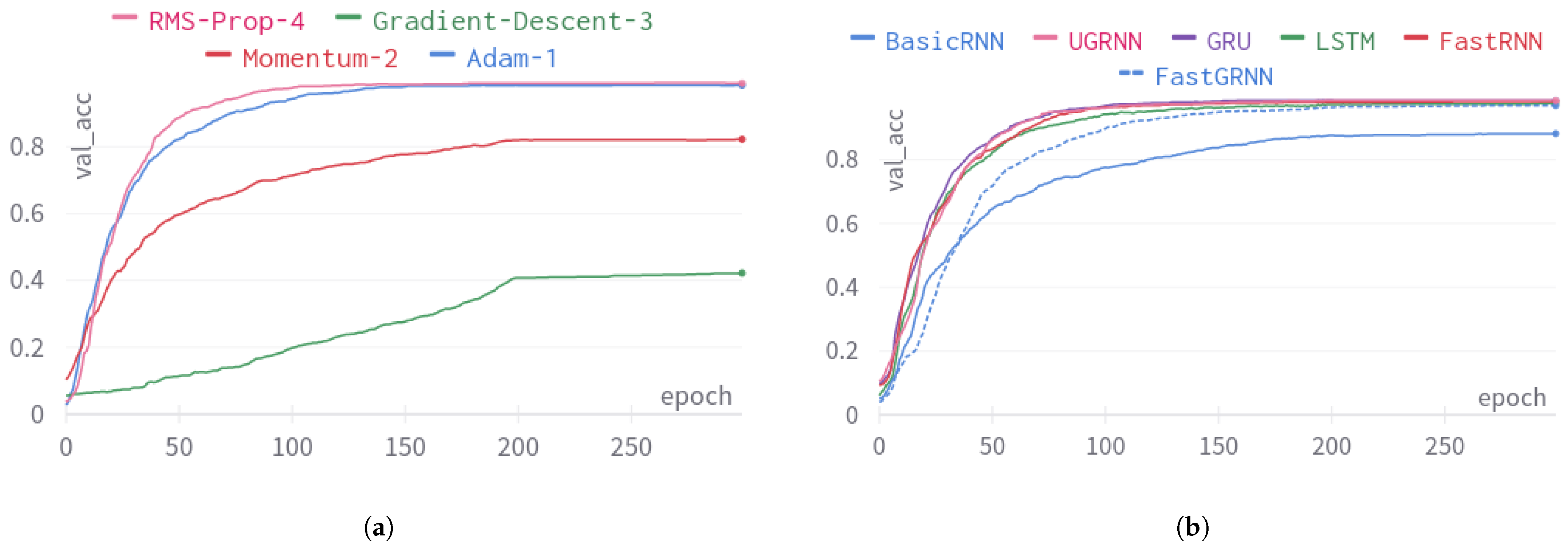
| SI No. | Dataset | Optimizer |
|---|---|---|
| 1 | DSA | Adam |
| 2 | SPHAR | RMS Prop |
| 3 | Opportunity | Adam |
| 4 | Pamap2 | Momentum Nesterov |
| 5 | MHEALTH | RMS Prop |
| 6 | USCHAD | RMS Prop |
| 7 | WHARF | Adam |
| 8 | WISDM | Adam |
| Compression Hyperparameters | Evaluation Metrics | Description | |||||||
|---|---|---|---|---|---|---|---|---|---|
| uRank | wRank | sU | sW |
Model_SIZE (KB) | train_acc | val_acc | Test_acc | F1 Score | |
| - | - | 1 | 1 | 5.20 | 0.99 | 0.97 | 0.98 | 0.98 | Baseline |
| 8 | 8 | 1 | 1 | 4.30 | 0.99 | 0.97 | 0.96 | 0.96 | Low-Rank Parameterization (LRP) |
| - | - | 0.9 | 0.9 | 5.00 | 0.99 | 0.98 | 0.98 | 0.98 | Hard thresholding and sparse retraining (HTSR) |
| 16 | 16 | 0.5 | 0.5 | 7.20 | 0.99 | 0.98 | 0.97 | 0.97 | Combination of both LRP and HTSR |
| 8 | 8 | 0.8 | 0.8 | 4.3 | 0.99 | 0.98 | 0.97 | 0.9732 | Memory efficient |
| 12 | 12 | 0.6 | 0.6 | 5.75 | 0.99 | 0.98 | 0.97 | 0.97 | Performance efficient |
| 5 | 5 | 0.9 | 0.9 | 3.2 | 0.98 | 0.97 | 0.96 | 0.96 | Our choice for performance and memory savings |
| 10 | 10 | 0.5 | 0.5 | 5.02 | 0.97 | 0.97 | 0.96 | 0.962 | Other trials |
| 7 | 7 | 0.9 | 0.9 | 3.93 | 0.98 | 0.97 | 0.95 | 0.95 | Other trails |
| Compression Hyperparameters | Evaluation Metrics | Description | |||||||
|---|---|---|---|---|---|---|---|---|---|
| uRank | wRank | sU | sW |
Model_Size
(KB) | train_acc | val_acc | test_acc | F1 Score | |
| - | - | 1 | 1 | 2.03 | 0.95 | 0.95 | 0.94 | 0.94 | Baseline |
| 8 | 8 | 1 | 1 | 2.25 | 0.93 | 0.93 | 0.935 | 0.93 | Low rank parameterization (LRP) |
| - | - | 0.9 | 0.9 | 2.03 | 0.94 | 0.94 | 0.93 | 0.94 | Hard thresholding and sparse retraining (HTSR) |
| 12 | 12 | 0.8 | 0.8 | 3.20 | 0.94 | 0.95 | 0.932 | 0.9346 | Combination of both LRP and HTSR |
| 8 | 8 | 0.9 | 0.9 | 1.88 | 0.93 | 0.93 | 0.92 | 0.92 | Our choice for performance and memory savings |
| 16 | 16 | 0.5 | 0.5 | 4.03 | 0.94 | 0.94 | 0.92 | 0.94 | Performance-efficient |
| 4 | 4 | 0.8 | 0.8 | 1.3 | 0.91 | 0.91 | 0.91 | 0.91 | Memory-efficient |
| 10 | 10 | 0.5 | 0.5 | 2.76 | 0.92 | 0.91 | 0.91 | 0.919 | Other trials |
| 12 | 12 | 0.4 | 0.4 | 2.61 | 0.93 | 0.94 | 0.92 | 0.93 | Other trails |
| SI No. | RNN Unit | Inference Model Weights and Biases with No Rank | Inference Model Weights and Biases with Low-Rank Parameterization |
|---|---|---|---|
| 1 | Basic RNN | W, U, Bh | W1, W2, U1, U2, Bh |
| 2 | FastGRNN | W, U, Bg, Bh, zeta, nu | W1, W2, U1, U2, Bg, Bh, zeta, nu |
| 3 | FastRNN | W, U, B, alpha, beta | W1, W2, U1, U2, B, alpha, beta |
| 4 | UGRNN | W1, W2, U1, U2, Bg, Bh | W, W1, W2, U, U1, U2, Bg, Bh |
| 5 | LSTM | W1, W2, W3, W4, U1, U2, U3, U4, Bf, Bi, Bo, Bc | W, W1, W2, W3, W4, U, U1, U2, U3, U4, Bf, Bi, Bo, Bc |
| 6 | GRU | W1, W2, W3, U1, U2, Br, Bg | W, W1, W2, W3, U, U1, U2, Br, Bg |
| RNN Cell | Hidden Units | DSA | SPHAR | ||||||
|---|---|---|---|---|---|---|---|---|---|
| Test Acc. (%) | F1 Score | Train Time (min) | Model Size (KB) | Test Acc. (%) | F1 Score | Train Time (min) | Model Size (KB) | ||
| BasicRNN | 8 | 0.75 | 0.73 | 4.48 | 2.86 | 0.74 | 0.72 | 2.61 | 1.02 |
| 16 | 0.84 | 0.83 | 4.93 | 4.23 | 0.84 | 0.83 | 2.51 | 1.80 | |
| 32 | 0.90 | 0.90 | 4.75 | 6.98 | 0.86 | 0.85 | 1.71 | 3.36 | |
| FastGRNN | 8 | 0.92 | 0.91 | 10.98 | 2.09 | 0.88 | 0.88 | 7.15 | 0.93 |
| 16 | 0.96 | 0.96 | 11.65 | 3.21 | 0.91 | 0.91 | 7.04 | 1.64 | |
| 32 | 0.97 | 0.97 | 8.98 | 5.46 | 0.94 | 0.93 | 5.62 | 3.08 | |
| FastRNN | 8 | 0.95 | 0.94 | 6.76 | 1.79 | 0.91 | 0.91 | 7.73 | 1.28 |
| 16 | 0.97 | 0.97 | 7.95 | 2.79 | 0.94 | 0.94 | 7.97 | 2.25 | |
| 32 | 0.98 | 0.98 | 6.54 | 4.79 | 0.94 | 0.94 | 7.95 | 4.19 | |
| UGRNN | 8 | 0.95 | 0.94 | 7.02 | 2.72 | 0.92 | 0.92 | 11.35 | 1.23 |
| 16 | 0.97 | 0.97 | 7.18 | 4.32 | 0.92 | 0.92 | 12.24 | 1.91 | |
| 32 | 0.98 | 0.98 | 10.49 | 7.50 | 0.94 | 0.95 | 12.66 | 3.66 | |
| GRU | 8 | 0.95 | 0.94 | 14.63 | 3.92 | 0.93 | 0.93 | 18.07 | 1.57 |
| 16 | 0.98 | 0.98 | 6.19 | 6.36 | 0.93 | 0.94 | 11.19 | 2.95 | |
| 32 | 0.99 | 0.98 | 10.30 | 11.23 | 0.93 | 0.93 | 9.18 | 5.70 | |
| LSTM | 8 | 0.90 | 0.90 | 12.33 | 6.28 | 0.91 | 0.91 | 13.13 | 1.60 |
| 16 | 0.98 | 0.98 | 9.52 | 10.37 | 0.94 | 0.94 | 13.60 | 3.04 | |
| 32 | 0.98 | 0.97 | 13.08 | 18.56 | 0.94 | 0.94 | 21.41 | 5.91 | |
| Best Performance | GRU with 32 hidden units | UGRNN with 32 hidden units | |||||||
| Least Model Size | FRNN, FGRNN | FRNN, FGRNN, BasicRNN | |||||||
| Memory savings via Fast Gates | with respect to GRU16, with respect to GRU32 | with respect to LSTM32, with respect to UGRNN32 | |||||||
| Performance deviation via Fast Gates | up to 4% | up to 7% | |||||||
| RNN Cell | Hidden Units | Opportunity | Pamap2 | ||||||
|---|---|---|---|---|---|---|---|---|---|
| Test Acc. (%) | F1 Score | Train Time (min) | Model Size (KB) | Test Acc. (%) | F1 Score | Train Time (min) | Model Size (KB) | ||
| Basic RNN | 8 | 0.84 | 0.25 | 12.14 | 6.70 | 0.45 | 0.39 | 6.46 | 2.83 |
| 16 | 0.86 | 0.34 | 4.19 | 8.70 | 0.60 | 0.52 | 8.91 | 3.98 | |
| 32 | 0.87 | 0.38 | 9.27 | 12.70 | 0.59 | 0.54 | 6.31 | 6.30 | |
| FastGRNN | 8 | 0.85 | 0.29 | 13.25 | 3.92 | 0.71 | 0.64 | 8.69 | 2.99 |
| 16 | 0.86 | 0.34 | 21.71 | 5.30 | 0.73 | 0.65 | 7.48 | 4.59 | |
| 32 | 0.86 | 0.42 | 14.89 | 8.05 | 0.73 | 0.67 | 8.05 | 6.93 | |
| FastRNN | 8 | 0.86 | 0.33 | 15.99 | 4.70 | 0.57 | 0.63 | 7.72 | 4.96 |
| 16 | 0.85 | 0.39 | 15.77 | 6.23 | 0.62 | 0.65 | 9.21 | 5.55 | |
| 32.00 | 0.87 | 0.44 | 18.66 | 9.29 | 0.69 | 0.67 | 8.49 | 8.62 | |
| UGRNN | 8 | 0.85 | 0.34 | 23.32 | 4.41 | 0.75 | 0.69 | 12.65 | 4.08 |
| 16 | 0.86 | 0.38 | 14.36 | 6.29 | 0.81 | 0.77 | 9.48 | 6.08 | |
| 32 | 0.86 | 0.44 | 26.49 | 8.77 | 0.69 | 0.66 | 8.49 | 8.62 | |
| GRU | 8 | 0.86 | 0.37 | 19.45 | 7.05 | 0.69 | 0.63 | 10.24 | 4.73 |
| 16 | 0.87 | 0.42 | 31.89 | 10.34 | 0.78 | 0.72 | 12.02 | 7.39 | |
| 32 | 0.87 | 0.47 | 30.15 | 16.90 | 0.80 | 0.80 | 22.82 | 11.55 | |
| LSTM | 8 | 0.86 | 0.39 | 20.72 | 5.48 | 0.67 | 0.59 | 19.78 | 4.42 |
| 16 | 0.87 | 0.46 | 16.37 | 10.16 | 0.57 | 0.50 | 16.51 | 7.17 | |
| 32 | 0.86 | 0.46 | 26.24 | 17.16 | 0.59 | 0.53 | 19.28 | 12.67 | |
| Best Performance | GRU, LSTM with 1632 hidden units | GRU with 32 hidden units | |||||||
| Smallest Model | FGRNN | FRNN, FGRNN, BasicRNN | |||||||
| Memory Savings via Fast Gates | with respect to GRU32, with respect to LSTM16 | with respect to UGRNN16, with respect to GRU32 | |||||||
| Performance Deviation via Fast Gates | up to 5% | around 13–16% | |||||||
| RNN Type | MHEALTH-FNOW | MHEALTH-SNOW | |||||||
|---|---|---|---|---|---|---|---|---|---|
| Mean Train Acc. | Mean Val Acc. | Test Acc. | F1 Score | Model Size | Mean Train Acc. | Mean Val Acc. | Test Acc. | F1 Score | |
| Basic RNN | 0.77 | 0.76 | 0.83 | 0.78 | 3.30 | 0.86 | 0.85 | 0.85 | 0.81 |
| FastGRNN | 0.86 | 0.85 | 0.93 | 0.92 | 3.37 | 0.97 | 0.97 | 0.98 | 0.98 |
| FastRNN | 0.99 | 0.99 | 0.99 | 0.99 | 3.30 | 0.99 | 0.99 | 0.99 | 0.99 |
| UGRNN | 0.85 | 0.82 | 0.90 | 0.87 | 5.42 | 0.96 | 0.96 | 0.96 | 0.96 |
| GRU | 1.00 | 0.98 | 0.99 | 0.99 | 8.30 | 0.99 | 0.98 | 0.99 | 0.99 |
| LSTM | 0.96 | 0.94 | 0.96 | 0.95 | 10.80 | 0.99 | 0.99 | 0.99 | 0.99 |
| Best Performance | FRNN and GRU | FRNN, GRU and LSTM | |||||||
| Smallest Model | FRNN and BasicRNN | FRNN, BasicRNN | |||||||
| Memory Savings via Fast Gates | with respect to GRU, with respect to LSTM | ||||||||
| Performance Deviation via Fast Gates | Nil | ||||||||
| RNN Type | USCHAD-FNOW | USCHAD-SNOW | |||||||
|---|---|---|---|---|---|---|---|---|---|
| Mean Train Acc. | Mean Val Acc. | Test Acc. | F1 Score | Model Size | Mean Train Acc. | Mean Val Acc. | Test Acc. | F1 Score | |
| Basic RNN | 0.51 | 0.51 | 0.53 | 0.44 | 2.23 | 0.51 | 0.51 | 0.49 | 0.29 |
| FastGRNN | 0.70 | 0.70 | 0.73 | 0.64 | 2.30 | 0.71 | 0.71 | 0.73 | 0.73 |
| FastRNN | 0.77 | 0.76 | 0.79 | 0.73 | 2.24 | 0.87 | 0.87 | 0.90 | 0.86 |
| UGRNN | 0.85 | 0.85 | 0.87 | 0.83 | 3.67 | 0.85 | 0.86 | 0.90 | 0.87 |
| GRU | 0.84 | 0.83 | 0.84 | 0.80 | 5.11 | 0.86 | 0.84 | 0.88 | 0.84 |
| LSTM | 0.75 | 0.75 | 0.70 | 0.64 | 6.55 | 0.79 | 0.76 | 0.74 | 0.67 |
| Best Performance | UGRNN | FastRNN | |||||||
| Smallest Model | FRNN, FGRNN, BasicRNN | FRNN, FGRNN, BasicRNN | |||||||
| Memory Savings via Fast Gates | with respect to UGRNN | ||||||||
| Performance Deviation via Fast Gates | up to 10% | up to 1% | |||||||
| RNN Type | WHARF-FNOW | WHARF-SNOW | |||||||
|---|---|---|---|---|---|---|---|---|---|
| Mean Train Acc. | Mean Val Acc. | Test Acc. | F1 Score | Model Size | Mean Train Acc. | Mean Val Acc. | Test Acc. | F1 Score | |
| Basic RNN | 0.49 | 0.49 | 0.44 | 0.27 | 2.05 | 0.51 | 0.51 | 0.50 | 0.30 |
| FastGRNN | 0.49 | 0.50 | 0.45 | 0.27 | 2.12 | 0.59 | 0.59 | 0.55 | 0.36 |
| FastRNN | 0.57 | 0.59 | 0.55 | 0.43 | 2.05 | 0.63 | 0.63 | 0.61 | 0.43 |
| UGRNN | 0.58 | 0.57 | 0.53 | 0.34 | 3.30 | 0.66 | 0.67 | 0.67 | 0.49 |
| GRU | 0.57 | 0.56 | 0.50 | 0.34 | 4.55 | 0.58 | 0.56 | 0.53 | 0.36 |
| LSTM | 0.53 | 0.52 | 0.48 | 0.31 | 5.80 | 0.59 | 0.59 | 0.57 | 0.37 |
| Best Performance | FRNN | UGRNN | |||||||
| Smallest Model | FRNN and BasicRNN | FRNN, BasicRNN | |||||||
| Memory Savings via Fast Gates | with respect to UGRNN | ||||||||
| Performance Deviation via Fast Gates | Nil | up to 6% | |||||||
| RNN Type | WISDM-FNOW | WISDM-SNOW | |||||||
|---|---|---|---|---|---|---|---|---|---|
| Mean Train Acc. | Mean Val Acc. | Test Acc. | F1 Score | Model Size | Mean Train Acc. | Mean Val Acc. | Test Acc. | F1 Score | |
| Basic RNN | 0.82 | 0.80 | 0.81 | 0.69 | 1.27 | 0.80 | 0.79 | 0.82 | 0.67 |
| FastGRNN | 0.81 | 0.81 | 0.81 | 0.69 | 1.72 | 0.83 | 0.83 | 0.84 | 0.72 |
| FastRNN | 0.82 | 0.82 | 0.82 | 0.72 | 1.66 | 0.84 | 0.84 | 0.85 | 0.76 |
| UGRNN | 0.93 | 0.92 | 0.93 | 0.89 | 2.90 | 0.87 | 0.88 | 0.89 | 0.82 |
| GRU | 0.88 | 0.87 | 0.88 | 0.82 | 4.15 | 0.97 | 0.96 | 0.97 | 0.95 |
| LSTM | 0.85 | 0.84 | 0.75 | 0.84 | 5.40 | 0.79 | 0.79 | 0.79 | 0.62 |
| Best Performance | UGRNN | GRU | |||||||
| Smallest Model | FRNN and BasicRNN | FRNN, and BasicRNN | |||||||
| Memory Savings via Fast Gates | with respect to UGRNN | with respect to GRU | |||||||
| Performance Deviation via Fast Gates | up to 17% | up to 19% | |||||||
| SPHAR | DSA | ||||
|---|---|---|---|---|---|
| SI No. | RNN Unit | Accuracy (%) | Model Size (KB) | Accuracy (%) | Model Size (KB) |
| 1 | Basic RNN | 91.31 | 29 | 71 | 20 |
| 2 | FastRNN | 94.50 | 29 | 84.14 | 97 |
| 3 | FastGRNN | 95.59 | 3 | 83.73 | 3.25 |
| 4 | UGRNN | 94.53 | 37 | 84.74 | 399 |
| 5 | LSTM | 93.62 | 71 | 84.84 | 270 |
| 6 | GRU | 93.65 | 74 | 84.84 | 526 |
Disclaimer/Publisher’s Note: The statements, opinions and data contained in all publications are solely those of the individual author(s) and contributor(s) and not of MDPI and/or the editor(s). MDPI and/or the editor(s) disclaim responsibility for any injury to people or property resulting from any ideas, methods, instructions or products referred to in the content. |
© 2024 by the authors. Licensee MDPI, Basel, Switzerland. This article is an open access article distributed under the terms and conditions of the Creative Commons Attribution (CC BY) license (https://creativecommons.org/licenses/by/4.0/).
Share and Cite
Lalapura, V.S.; Bhimavarapu, V.R.; Amudha, J.; Satheesh, H.S. A Systematic Evaluation of Recurrent Neural Network Models for Edge Intelligence and Human Activity Recognition Applications. Algorithms 2024, 17, 104. https://doi.org/10.3390/a17030104
Lalapura VS, Bhimavarapu VR, Amudha J, Satheesh HS. A Systematic Evaluation of Recurrent Neural Network Models for Edge Intelligence and Human Activity Recognition Applications. Algorithms. 2024; 17(3):104. https://doi.org/10.3390/a17030104
Chicago/Turabian StyleLalapura, Varsha S., Veerender Reddy Bhimavarapu, J. Amudha, and Hariram Selvamurugan Satheesh. 2024. "A Systematic Evaluation of Recurrent Neural Network Models for Edge Intelligence and Human Activity Recognition Applications" Algorithms 17, no. 3: 104. https://doi.org/10.3390/a17030104
APA StyleLalapura, V. S., Bhimavarapu, V. R., Amudha, J., & Satheesh, H. S. (2024). A Systematic Evaluation of Recurrent Neural Network Models for Edge Intelligence and Human Activity Recognition Applications. Algorithms, 17(3), 104. https://doi.org/10.3390/a17030104