Inverse Kinematics of Robotic Manipulators Based on Hybrid Differential Evolution and Jacobian Pseudoinverse Approach

Abstract

Robot manipulators play a critical role in several industrial applications by providing high precision and accuracy. To perform these tasks, manipulator robots require the effective computation of inverse kinematics. Conventional methods to solve IK often encounter significant challenges, such as singularities, non-linear equations, and poor generalization across different robotic configurations. In this work, we propose a novel approach to solve the inverse kinematics (IK) problem in robotic manipulators using a metaheuristic algorithm enhanced with a Jacobian step. Our method overcomes those limitations by selectively applying the Jacobian step to the differential evolution (DE) algorithm. The effectiveness and versatility of the proposed approach are demonstrated through simulations and real-world experimentation on a 5 DOF KUKA robotic arm.

1. Introduction

Manipulator robots, known for their unparalleled precision, efficiency, and safety, are revolutionizing industries across the globe. These versatile machines are pivotal in space applications, where they service satellites, remove orbital debris, and construct and maintain orbital assets, ensuring the sustainability of our extraterrestrial endeavors [1]. In the automotive industry, robotic manipulators excel in welding tasks, utilizing an electric arc and shielding gas to enhance manufacturing processes [2]. The healthcare sector has also benefited immensely, with robotic arms enabling minimally invasive surgeries that surpass traditional open surgery methods in terms of precision and recovery time [3]. By performing repetitive and hazardous tasks with consistent accuracy, these robotic systems not only improve operational efficiency but also ensure worker safety. Central to their functionality is the complex challenge of solving the inverse kinematics (IK) of the robotic manipulator, a crucial aspect that underpins their application in these diverse fields.

The inverse kinematics problem entails determining the joint variable configuration that corresponds to a specific position and orientation of the end-effector. This task is generally more complex than solving the forward kinematics problem for several reasons [4]:

• Equations to solve are generally non-linear, making it not always possible to find a closed-form solution.
• Multiple solutions may exist.
• Infinite solutions may exist.
• There might be no admissible solutions.

Conventional numerical methods based on differential kinematics rely on the Jacobian matrix to determine the relationship between joint variables and end-effector positions [5]. However, these methods encounter significant problems due to singularities in the Jacobian matrix, which can lead to undefined or infinite solutions [4,6]. Closed-form methods such as algebraic or geometric methods are commonly used for manipulators with simple geometric structures [7]. Due to these drawbacks, artificial intelligence methods are increasingly utilized to solve the inverse kinematics problem.

In recent years, although to a limited extent, the solution of inverse kinematics has been explored using Artificial Neural Networks (ANNs). Typically, the input to the network is the desired position and orientation of the end-effector and the output is the vector of generalized coordinates, representing the robot’s joint configurations. However, this method faces challenges in generalizing across different kinematic structures or manipulators, as it requires a unique dataset for each specific manipulator. Due to the complexity of the problem, research has been limited to solving it within the three-dimensional Cartesian plane, with the additional necessity of identifying singularity zones [8,9]. Additionally, approaches that account for both position and rotation demand very large datasets and an optimization process for the candidate solution, often utilizing numerical methods such as the Newton–Raphson method [10].

For these reasons, this paper proposes solving the inverse kinematics problem using metaheuristic algorithms. In the past decade, metaheuristic algorithms have emerged as a viable alternative for addressing various challenges in robotics. These algorithms are particularly useful for solving problems that are difficult to tackle with conventional methods or for which no exact solution method exists [11]. In the literature we can find examples of the application of metaheuristic algorithms, such as their use for hyperparameter tuning in both machine learning algorithms and deep neural networks [12], and trajectory tracking optimization [13], as well as in robotic navigation [14].

A review of the state of the art in robotic applications, particularly addressing the inverse kinematics of manipulator robots, is presented in

Table 1. State of the art related work.

Reference	Algorithm	DOFs	Orientation	Boundaries	Robot Application
[15]	PSO	5,6-DOF	✓	✓	✗
[16]	DE	6,7,8,9-DOF	✓	✓	✓
[17]	PSO, multi-PSP, imp PSO	6-DOF	✓	✓	✗
[18]	DE	5-DOF	✗	✓	✗
[19]	DE	6-DOF	✓	✓	✗
[20]	PSO	6-DOF	✓	✓	✗
[21]	ABC	6-DOF	✗	✓	✗
[22]	BA	6-DOF	✗	✓	✗
[23]	PSO	7-DOF	✗	✓	✗
[24]	FA	5-DOF	✗	✓	✗
[25]	$\beta -SSA$	6,8-DOF	✗	✓	✗
[26]	Modified DE	10-DOF	✗	✗	✗
[27]	GWO	6-DOF	✗	✓	✗
[28]	GMO	6-DOF	✓	✗	✗
Proposed Method	DE-H	5,6,7-DOF	✓	✓	✓

. This review highlights that differential evolution (DE) and particle swarm optimization (PSO) are the most commonly used metaheuristic algorithms for solving the inverse kinematics problem. Other algorithms, such as Artificial Bee Colony (ABC), bees algorithm (BA), Beta Salp Swarm Algorithm ($\beta$-SSA), Wild Geese Migration Optimization (GMO), Gray Wolf Optimization (GWO), and Firefly Algorithm (FA), have also been implemented. Most studies focus on a single manipulator, with only two cases [15,16] proposing more generalized methods. Typically, these studies address only the position problem, as incorporating orientation significantly increases the complexity of solving the inverse kinematics. Although joint limits are considered in all optimization processes, hard bounding is commonly applied to manage constraints, or candidate solutions are recalculated when they exceed the search space. This approach is necessary because metaheuristic algorithms are not inherently designed to handle constrained problems.

In this paper, we propose a novel method to solve inverse kinematics using a metaheuristic algorithm combined with a Jacobian step. Unlike traditional approaches, the Jacobian step is applied neither in each iteration nor to a subpopulation; it is used selectively when a deadlock is detected, and only to the global best solution. This strategy reduces the implementation complexity of the algorithm. Our method effectively addresses both position and orientation in inverse kinematics, formulating the problem as a constrained optimization task where joint limits are represented as constraints. Since metaheuristic algorithms are not inherently designed for constrained problems, we employ penalty functions to manage these constraints. Our approach is generalizable to redundant robots with n degrees of freedom. The applicability of the algorithm is demonstrated using a 5 DOF KUKA robotic arm, showcasing its effectiveness and versatility.

A comparative study is conducted using the following metaheuristic algorithms: the differential evolution algorithm “DE” proposed by storn et al. in 1997 [29], the particle swarm optimization algorithm “PSO” proposed by Kennedy and Heberhart in 1995 [30], the bees algorithm “BA” proposed by Pham et al. in 2006 [31], the invasive weed optimization algorithm “IWO” proposed by Mehrabian and Lucas in 2006 [32] and the imperialist competitive algorithm “ICA” proposed by Atashpaz-Gargari and Lucas in 2007 [33].

2. Robot Manipulator Kinematics

A robot manipulator consist of a series of links interconnected by joints, forming a kinematic chain. The beginning of the chain is fixed to a base and an end-effector tool is connected to the end of the chain. A joint variable $\mathbf{q}$ is defined as $\mathbf{q}={\left[\begin{array}{cccc}{q}_1& q_2& \cdots & q_n\end{array}\right]}^T$ where each joint $q_j$ with $j=1,2,\cdots ,n$, where n represents the total DOFs of the manipulator robot [4,34].

A manipulator kinematics model can be described based on the Denavit–Hartenberg convention (DH). Since each joint connects two links, a robot manipulator with n joints will have $n+1$ links. In the DH convention, joint i connects link $i-1$ to link i. Each link i is represented by a homogenous matrix ${}^{i-1}\mathbf{T}_i$ that transforms the frame attached to the link $i-1$ into the joint link i. The homogeneous matrix ${}^{i-1}\mathbf{T}_i$ is defined as

$${}^{i-1}\mathbf{T}_i=\left[\begin{array}{cccc}\hfill cos{\theta }_i& -sin{\theta }_{i}cos{\alpha }_i& \hfill sin{\theta }_{i}sin{\alpha }_i& a_{i}cos{\theta }_i\\ \hfill sin{\theta }_i& cos{\theta }_{i}cos{\alpha }_i& \hfill -cos{\theta }_{i}sin{\alpha }_i& a_{i}sin{\theta }_i\\ \hfill 0& \hfill sin{\alpha }_i& \hfill cos{\alpha }_i& \hfill d_i\\ \hfill 0& \hfill 0& \hfill 0& \hfill 1\end{array}\right],$$

(1)

where the parameters ${\theta }_i$, $a_i$, $d_i$, and ${\alpha }_i$ represent the joint angle, link length, link offset, and link twist, respectively. The parameter ${\theta }_i=q_i$ becomes the joint variable for revolute joints. In contrast, the parameter $d_i=q_i$ becomes the joint variable for prismatic joints. In both cases, the rest of the parameters remain constant.

The forward kinematics computes the end-effector pose ${}^0\mathbf{T}_n$ given the joint variable $\mathbf{q}$ which is

$${}^0\mathbf{T}_n\left(\mathbf{q}\right)=\prod _{i=1}^n{}^{i-1}\mathbf{T}_i\left(q_i\right).$$

(2)

The end-effector pose ${}^0\mathbf{T}_n$ contains the position $\mathbf{t}$ and orientation $\mathbf{R}$ of the tool in the following form:

$${}^0\mathbf{T}_n\left(\mathbf{q}\right)=\left[\begin{array}{cc}\mathbf{R}\left(\mathbf{q}\right)& \mathbf{t}\left(\mathbf{q}\right)\\ \mathbf{0}& 1\end{array}\right]=\left[\begin{array}{cccc}{r}_{11}& r_{12}& r_{13}& t_x\\ r_{21}& r_{22}& r_{23}& t_y\\ r_{31}& r_{32}& r_{33}& t_z\\ 0& 0& 0& 1\end{array}\right].$$

(3)

The inverse kinematics computes the joint variable $\mathbf{q}$ given the end-effector pose ${}^0\mathbf{T}_n$. The iterative Jacobian pseudoinverse algorithm can solve the inverse kinematics as follows:

$${\mathbf{q}}_{k+1}={\mathbf{q}}_k+\lambda {\mathbf{J}}^{†}\left({\mathbf{q}}_k\right)\mathbf{e}\left({\mathbf{q}}_k\right),$$

(4)

where k represents the current iteration, $\lambda$ is a positive scalar factor with $\lambda >0$, $\mathbf{J}\in {\mathbb{R}}^{6\times n}$ is a Jacobian matrix, and $\mathbf{e}\left({\mathbf{q}}_k\right)$ is an error between a desired and current end-effector pose. Moreover, the operation ${\mathbf{J}}^{†}$ is the pseudoinverse of $\mathbf{J}$ also called the Moore–Penrose inverse. For manipulators of 6 DOF ($n=6$), ${\mathbf{J}}^{-1}$ is rather used. The error $\mathbf{e}\left({\mathbf{q}}_k\right)$ is defined as

$$\mathbf{e}\left({\mathbf{q}}_k\right)={\left[\begin{array}{cc}{\mathbf{e}}_v\left({\mathbf{q}}_k\right)& {\mathbf{e}}_{\omega }\left({\mathbf{q}}_k\right)\end{array}\right]}^T,$$

(5)

where ${\mathbf{e}}_v\left({\mathbf{q}}_k\right)$ is the translation error between the desired ${\mathbf{t}}_d$ and current $\mathbf{t}\left({\mathbf{q}}_k\right)$ end-effector position. This error is defined as

$${\mathbf{e}}_v\left({\mathbf{q}}_k\right)={\mathbf{t}}_d-\mathbf{t}\left({\mathbf{q}}_k\right).$$

(6)

Moreover, ${\mathbf{e}}_{\omega }\left({\mathbf{q}}_k\right)$ is the orientation error between the desired ${\mathbf{R}}_d$ and current $\mathbf{R}\left({\mathbf{q}}_k\right)$ orientation, that is,

$${\mathbf{e}}_{\omega }\left({\mathbf{q}}_k\right)={\displaystyle \frac{1}{2}}\left[\left(\mathbf{R}\left({\mathbf{q}}_k\right)\left[\begin{array}{c}1\\ 0\\ 0\end{array}\right]\times {\mathbf{R}}_d\left[\begin{array}{c}1\\ 0\\ 0\end{array}\right]\right)+\left(\mathbf{R}\left({\mathbf{q}}_k\right)\left[\begin{array}{c}0\\ 1\\ 0\end{array}\right]\times {\mathbf{R}}_d\left[\begin{array}{c}0\\ 1\\ 0\end{array}\right]\right)+\left(\mathbf{R}\left({\mathbf{q}}_k\right)\left[\begin{array}{c}0\\ 0\\ 1\end{array}\right]\times {\mathbf{R}}_d\left[\begin{array}{c}0\\ 0\\ 1\end{array}\right]\right)\right].$$

(7)

The forward kinematics always provide a solution for any joint variable $\mathbf{q}$. However, inverse kinematics may yield multiple solutions for the same end-effector pose ${}^0\mathbf{T}_n$. Additionally, the equations involved to solve the inverse kinematics are non-linear, and for that reason it is not always possible to find a closed-form solution. The iterative Jacobian pseudoinverse method is a commonly used approach for solving inverse kinematics. However, this method is prone to singularities, as it necessitates the inversion of a Jacobian matrix that can become rank deficient. To address these limitations, this work proposes solving the inverse kinematics problem using metaheuristic algorithms.

3. Differential Evolution

Differential evolution (DE) is a population-based algorithm employed for global optimization. In this algorithm, population members are called individuals and they represent potential solutions. These individuals are adjusted during an iterative process (generations) by performing three principal operations: mutation, crossover, and selection.

Initially, each individual ${\mathbf{x}}_i^G={\left[\begin{array}{cccc}{x}_{i,1}^G& x_{i,2}^G& \cdots & x_{i,D}^G\end{array}\right]}^T$ is randomly generated, where $i=1,2,3,\cdots ,N$ with N representing the total number of population members, D denoting the dimension of the problem, and G indicating the current generation.

The mutation operation generates a mutant vector ${\mathbf{v}}_i^G={\left[\begin{array}{cccc}{v}_{i,1}^G& v_{i,2}^G& \cdots & v_{i,D}^G\end{array}\right]}^T$ as follows:

$${\mathbf{v}}_i^G={\mathbf{x}}_{r_1}^G+F\left({\mathbf{x}}_{r_2}^G-{\mathbf{x}}_{r_3}^G\right),$$

(8)

where ${\mathbf{x}}_{r_1}^G$, ${\mathbf{x}}_{r_2}^G$, and ${\mathbf{x}}_{r_3}^G$ are individuals chosen randomly such that $r_1,r_2,r_3\in \left\{1,N\right\}$ and $i\ne r_1\ne r_2\ne r_3$. Moreover, $F\in \left[0,2\right]$ is called the amplification factor.

A trial vector ${\mathbf{u}}_i^G={\left[\begin{array}{cccc}{u}_{i,1}^G& u_{i,2}^G& \cdots & u_{i,D}^G\end{array}\right]}^T$ is created by the following crossover operation:

$$u_{i,j}^G=\left\{\begin{array}{cc}{v}_{i,j}^G\hfill & \mathbf{if}r\le C_R\mathbf{or}j=r_j\hfill \\ x_{i,j}^G\hfill & \mathbf{if}r>C_R\mathbf{and}j\ne r_j,\hfill \end{array}\right.$$

(9)

where $C_R\in [0,1]$ is the crossover constant, and $r\in [0,1]$ and $r_j\in \left\{1,D\right\}$ are random numbers.

In the selection operation, the trial vector ${\mathbf{u}}_i^G$ is compared to the current vector ${\mathbf{x}}_i^G$ according to the following scheme:

$${\mathbf{x}}_i^{G+1}=\left\{\begin{array}{cc}{\mathbf{u}}_i^G\hfill & \mathbf{if}f\left({\mathbf{u}}_i^G\right)<f\left({\mathbf{x}}_i^G\right)\hfill \\ {\mathbf{x}}_i^G\hfill & \mathbf{otherwise},\hfill \end{array}\right.$$

(10)

where f is an objective function. Trial vector ${\mathbf{u}}_i^G$ replaces ${\mathbf{x}}_i^{G+1}$ if ${\mathbf{u}}_i^G$ yields a better solution; otherwise, ${\mathbf{x}}_i^G$ is retained in the next iteration. A detailed description of DE can be found in [29].

4. Approach Description

This section presents a comprehensive description of the objective function formulation and introduces the algorithm for solving inverse kinematics using a hybrid differential evolution approach.

4.1. Objective Function Formulation

This work proposes solving the inverse kinematics (IK) problem as a global constrained optimization task. The objective function is formulated to minimize the error between the desired end-effector pose $\left({\mathbf{R}}_d,{\mathbf{t}}_d\right)$ and the current end-effector pose $\left(\mathbf{R}\left(\mathbf{q}\right),\mathbf{t}\left(\mathbf{q}\right)\right)$, which can be computed using Equations (2) and (3).

The objective function f is defined as

$$f\left(\mathbf{q}\right)=k_t∥{\mathbf{t}}_d-\mathbf{t}\left(\mathbf{q}\right)∥+k_R∥{\mathbf{R}}_d-\mathbf{R}\left(\mathbf{q}\right)∥,$$

(11)

where $∥{\mathbf{t}}_d-\mathbf{t}\left(\mathbf{q}\right)∥$ represents a Euclidean norm error between the desired and the current position, and $∥{\mathbf{R}}_d-\mathbf{R}\left(\mathbf{q}\right)∥$ represents the Frobenius norm error between the desired and the current orientation. Additionally, $k_t$ and $k_R$ are positive weight factors.

The optimization problem is then defined as follows:

$$\begin{array}{c}\underset{\mathbf{q}}{arg\; min}f\left(\mathbf{q}\right),\mathrm{subject}\mathrm{to}{\mathbf{q}}_l<\mathbf{q}<{\mathbf{q}}_u,\end{array}$$

(12)

where ${\mathbf{q}}_l$ and ${\mathbf{q}}_u$ are the lower and upper joint boundary, respectively. The joint boundary represents the joint limits. They are defined as

$$\begin{array}{cc}\hfill {\mathbf{q}}_l& ={\left[\begin{array}{cccc}{q}_{l,1}& q_{l,2}& \cdots & q_{l,n}\end{array}\right]}^T,\\ \hfill {\mathbf{q}}_u& ={\left[\begin{array}{cccc}{q}_{u,1}& q_{u,2}& \cdots & q_{u,n}\end{array}\right]}^T.\end{array}$$

The constrained optimization in (12) is reformulated as an unconstrained optimization problem using quadratic penalty functions. The proposed objective function $f^{\prime }\left(\mathbf{q}\right)$ is then defined as follows:

$$f^{\prime }\left(\mathbf{q}\right)=f\left(\mathbf{q}\right)+\gamma \left[\sum _{j=1}^{n}max{\left(0,q_{l,j}-q_j\right)}^2+\sum _{j=1}^{n}max{\left(0,q_j-q_{u,j}\right)}^2\right],$$

(13)

where $\gamma >0$ is a coefficient that scales the contribution of the penalty functions. By setting $\gamma$ larger, constraints are penalized more severely. Moreover, when $q_{l,j}-q_j\le 0$ and $q_j-q_{u,j}\le 0$, the constraint in dimension j is satisfied.

Finally, the proposed optimization problem is given as

$$\underset{\mathbf{q}}{arg\; min}{f}^{\prime }\left(\mathbf{q}\right).$$

(14)

Notice that the proposed objective function (13) incorporates the weighted error in both position and orientation, along with a penalty scheme. By minimizing the objective function, the joint configurations result in lower position and orientation errors while ensuring feasible joint solutions.

4.2. Inverse Kinematics Using Hybrid Differential Evolution

We propose enhancing the exploitation of differential evolution (DE) with Jacobian-based refinements, tracking the improvements of the best individuals over generations. If the position of the best individual stagnates, a Jacobian pseudoinverse step is performed to generate a candidate solution. This candidate solution replaces the current best individual if it provides a better solution. This operation enhances the local exploitation capabilities of DE with Jacobian-based refinements while preserving the exploration capabilities of DE.

The best individual is considered to be stagnating when there is not improvement after several generations. An $l^G$ counter tracks the number of consecutive unsuccessful modifications at generation G. If $l^G$ reaches a predefined stagnation limit L, a Jacobian-based refinement is performed. This process is called the Jacobian pseudoinverse step.

The Jacobian pseudoinverse step produces a candidate solution based on the conventional numerical method (4). The candidate solution ${\mathbf{w}}_g^G$ is generated as follows:

$${\mathbf{w}}_g^G={\mathbf{x}}_g^G+{\mathbf{J}}^{†}\left({\mathbf{x}}_g^G\right)\mathbf{e}\left({\mathbf{x}}_g^G\right),$$

(15)

where ${\mathbf{x}}_g^G$ denotes the best individual at generation G. The candidate solution is then compared against the current best solution according to the following scheme:

$${\mathbf{x}}_g^{G+1}=\left\{\begin{array}{cc}{\mathbf{w}}_g^G\hfill & \mathbf{if}f\left({\mathbf{w}}_g^G\right)<f\left({\mathbf{x}}_g^G\right)\hfill \\ {\mathbf{x}}_g^G\hfill & \mathbf{otherwise},\hfill \end{array}\right.$$

(16)

which is a selection operation. If candidate solution ${\mathbf{w}}_g^G$ produces a better solution than ${\mathbf{x}}_g^G$, ${\mathbf{w}}_g^G$ replaces the best individual for the next generation. Otherwise, ${\mathbf{x}}_g^G$ is retained.

4.3. Proposed Algorithm

The proposed inverse kinematics algorithm, based on hybrid differential evolution, is outlined in Algorithm 1. Initially, individuals are generated randomly based on the following operation:

$$x_{i,j}=q_{l,j}+r\left(q_{u,j}-q_{l,j}\right)$$

(17)

where $r\in [0,1]$ is a random number.

The algorithm performs the mutation, recombination, and selection operation on each individual in the population. Subsequently, the algorithm identifies the best individual ${\mathbf{x}}_g^G$. It then checks whether the best individual has stagnated, determined by whether the stagnation counter $l^G$ exceeds the predefined limit L (i.e., $l^G>L$). If stagnation is detected, the proposed Jacobian pseudoinverse operation is performed. In this scenario, a candidate solution ${\mathbf{w}}_g^G$ is computed using the Jacobian pseudoinverse step. Local refinements are made if ${\mathbf{w}}_g^G$ proves to be a better solution than ${\mathbf{x}}_g^G$. Additionally, the stagnation counter $l^G>L$ increases when $f^{\prime }\left({\mathbf{x}}_g^{G+1}\right)<f^{\prime }\left({\mathbf{x}}_g^G\right)$, indicating an unsuccessful improvement. This process is repeated until the stopping criteria are met. Finally the algorithm returns the individual with the best fitness as the solution.

Algorithm 1 Proposed inverse kinematics based on hybrid differential evolution.

1: set objective function $f^{\prime }$ as in (13) 2: set $F\in [0,2]$ and $C_R\in [0,1]$ values 3: set joint boundary ${\mathbf{q}}_l$ and ${\mathbf{q}}_u$ 4: set stagnation counter $l=0$ and stagnation limit L 5: for each individual i do 6:       for each dimension j do 7:             randomly compute $r\in [0,1]$ 8:             $x_{i,j}=q_{l,j}+r\left(q_{u,j}-q_{l,j}\right)$ 9:       end 10: end 11: repeat 12:       // Mutation, recombination, and selection operations on population: 13:       for each individual i do 14:             randomly choose $r_1,r_2,r_3$, such that $i\ne r_1\ne r_2\ne r_3$ 15:             ${\mathbf{v}}_i^G={\mathbf{x}}_{r_1}^G+F\left({\mathbf{x}}_{r_2}^G-{\mathbf{x}}_{r_3}^G\right)$ 16:             randomly compute $r_j\in \left\{1,D\right\}$ 17:             for each dimension j do 18:                   randomly compute $r\in [0,1]$ 19:                   if r $\le C_R$ or $j=r_j$ then 20:                         $u_{i,j}^G=v_{i,j}^G$ 21:                   otherwise 22:                         $u_{i,j}^G=x_{i,j}^G$ 23:                   end 24:             end 25:             if $f^{\prime }\left({\mathbf{u}}_i^G\right)<f^{\prime }\left({\mathbf{x}}_i^G\right)$ then 26:                   ${\mathbf{x}}_i^{G+1}={\mathbf{u}}_i^G$ 27:             end 28:       end 29:       // Jacobian pseudoinverse operation: 30:       find best individual g 31:       if $l^G>L$ then 32:             ${\mathbf{w}}_g^G={\mathbf{x}}_g^G+{\mathbf{J}}^{†}\left({\mathbf{x}}_g^G\right)\mathbf{e}\left({\mathbf{x}}_g^G\right)$ 33:             if $f^{\prime }\left({\mathbf{w}}_g^G\right)<f^{\prime }\left({\mathbf{x}}_g^G\right)$ 34:                   ${\mathbf{x}}_g^{G+1}={\mathbf{w}}_g^G$ 35:             otherwise 36:                   ${\mathbf{x}}_g^{G+1}={\mathbf{x}}_g^G$ 37:             end 38:             $l^G=0$ 39:       end 40:       if $f^{\prime }\left({\mathbf{x}}_g^{G+1}\right)<f^{\prime }\left({\mathbf{x}}_g^G\right)$ then 41:             $l^{G+1}=0$ 42:       otherwise 43:             $l^{G+1}=l^G+1$ 44:       end 45: until the stopping criteria are met 46: Return the individual with the best fitness as the solution

5. Simulation and Experimental Results

Experiments aim to test the proposed inverse kinematics algorithm under different manipulator structures. Simulations perform a comparison among metaheuristic algorithms. Moreover, real-world experiments validate the applicability of the proposal.

5.1. Simulation Experiments

The objective of these simulations is to compare the performance of various metaheuristic algorithms—BA (BA), differential evolution (DE), particle swarm optimization (PSO), invasive weed optimization (IWO), and the imperialist competitive algorithm (ICA)—in solving the inverse kinematics for both the position and orientation of the Puma 560 robot (6 DOF), Baxter robot (7 DOF), and KUKA iiwa robot (7 DOF). Moreover, simulations are performed using Matlab R2024b.

Each simulation consists of $G=300$ iterations and a population of $N=30$ individuals. The following parameters were defined: $k_t=1.5$, $k_R=0.8$, $\gamma =1000$, $C_R=0.9$, and $F=0.6$; the Denavit–Hartenberg (DH) convention was used to describe the kinematic structure of the manipulators used in the simulations.

Table 2. Puma-560 manipulator DH parameters.

Joint	a [m]	$\mathit{\alpha }$ [rad]	d [m]	$\mathbf{\Theta }$ [rad]
1	0	$\pi /2$	0	$q_1$
2	0.4318	0	0	$q_2$
3	0.0203	$-\pi /2$	0.15	$q_3$
4	0	$\pi /2$	0.4318	$q_4$
5	0	$-\pi /2$	0	$q_5$
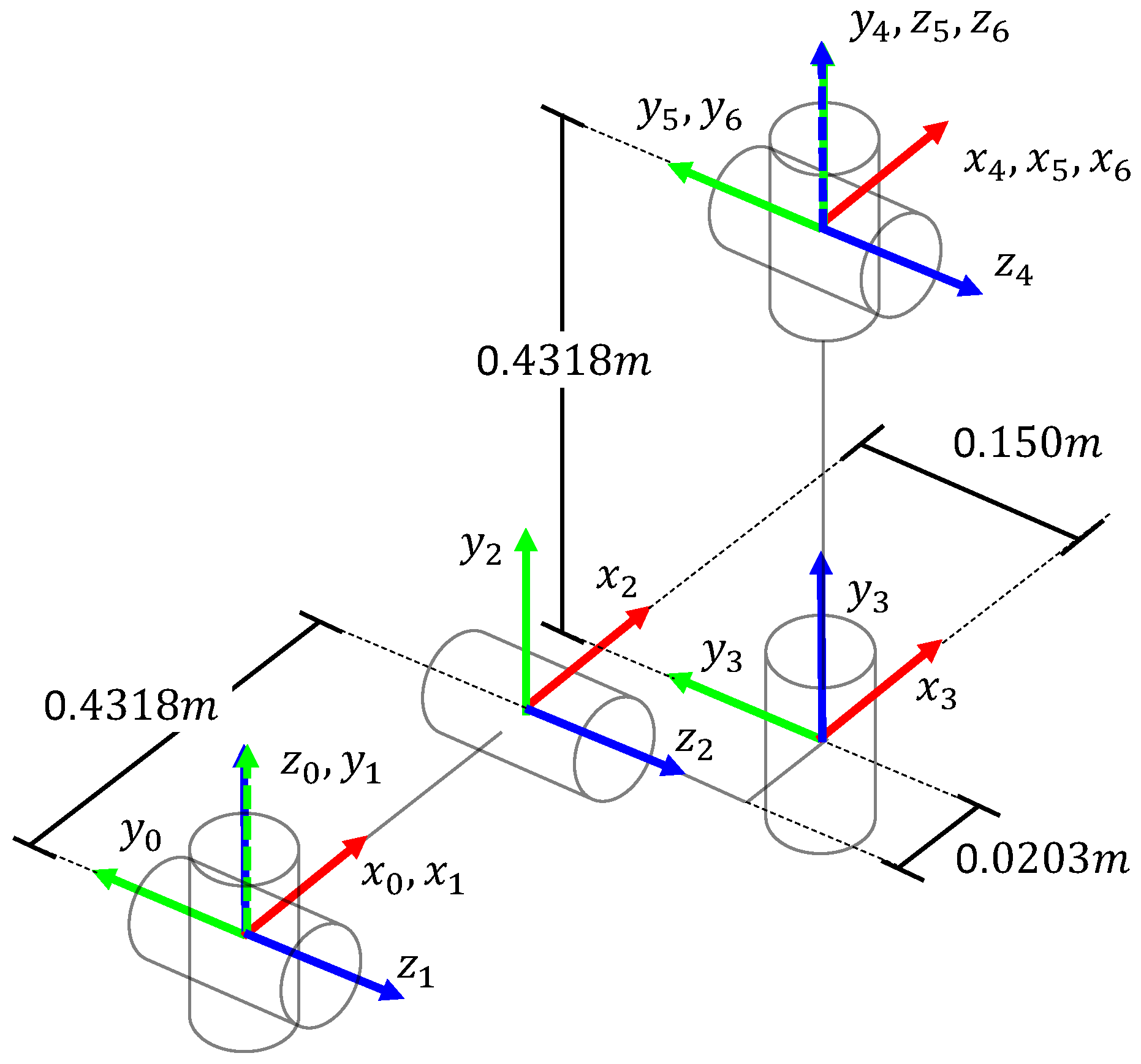
6	0	0	0	$q_6$

presents the DH parameters for the Puma-560 manipulator.

Table 3. Baxter manipulator DH parameters.

Joint	a [m]	$\mathit{\alpha }$ [rad]	d [m]	$\mathbf{\Theta }$ [rad]
1	0.069	$-\pi /2$	0.270	$q_1$
2	0	$\pi /2$	0	$q_2$
3	0.069	$-\pi /2$	0.364	$q_3$
4	0	$\pi /2$	0	$q_4$
5	0.01	$-\pi /2$	0.374	$q_5$
6	0	$\pi /2$	0	$q_6$
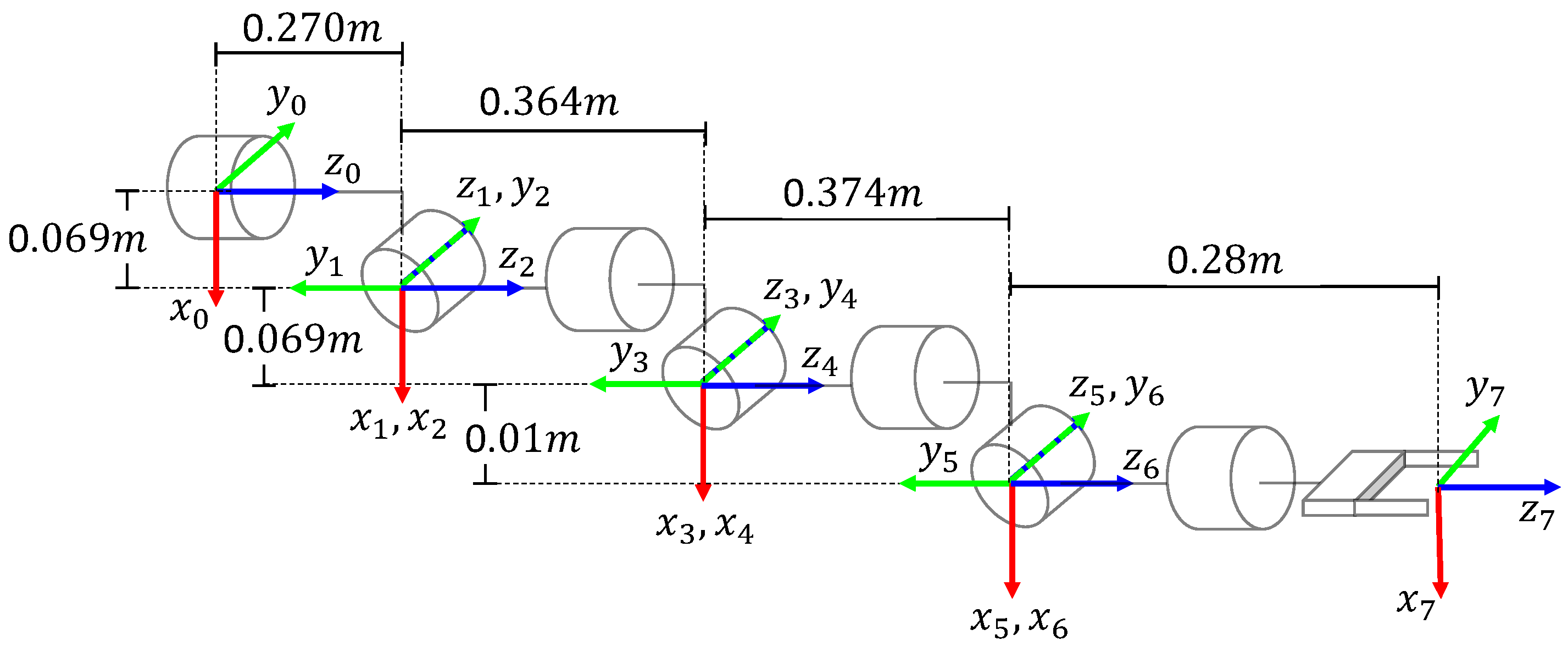
7	0	0	0.28	$q_7$

provides the DH parameters of the Baxter manipulator.

Table 4. KUKA iiwa manipulator DH parameters.

Joint	a [m]	$\mathit{\alpha }$ [rad]	d [m]	$\mathbf{\Theta }$ [rad]
1	0	$-\pi /2$	0.360	$q_1$
2	0	$\pi /2$	0	$q_2$
3	0	$\pi /2$	0.420	$q_3$
4	0	$-\pi /2$	0	$q_4$
5	0	$-\pi /2$	0.400	$q_5$
6	0	$\pi /2$	0	$q_6$
7	0	0	0.126	$q_7$

lists the DH parameters for the KUKA iiwa manipulator. Moreover, the illustrations in Figure 1, Figure 2 and Figure 3 show the coordinate frames’ assignment for the considered manipulators.

The joint limits for the Puma-560 robot are as follows:

$${\mathbf{q}}_l={\left[\begin{array}{cccccc}-160& -45& -225& -110& -100& -266\end{array}\right]}^T$$

$${\mathbf{q}}_u={\left[\begin{array}{cccccc}160& 225& 45& 170& 100& 266\end{array}\right]}^T$$

The joint limits for the Baxter robot are as follows:

$${\mathbf{q}}_l={\left[\begin{array}{ccccccc}-97.5& -123& -175& -3& -175& -90& -175\end{array}\right]}^T$$

$${\mathbf{q}}_u={\left[\begin{array}{ccccccc}97.5& 60& 175& 150& 175& 120& 175\end{array}\right]}^T$$

The joint limits for the KUKA iiwa robot are as follows:

$${\mathbf{q}}_l={\left[\begin{array}{ccccccc}-170& -120& -170& -120& -170& -120& -175\end{array}\right]}^T$$

$${\mathbf{q}}_u={\left[\begin{array}{ccccccc}170& 120& 170& 120& 170& 120& 175\end{array}\right]}^T$$

In all cases, the equivalent values in radians are used in the algorithms.

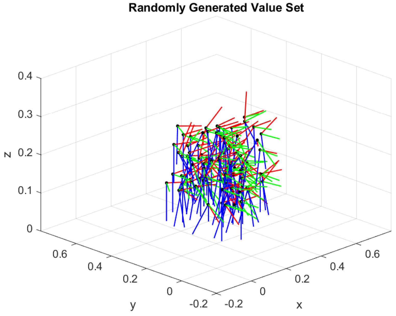
The desired end-effector poses are defined with a set of 100 random positions and orientations generated in a valid workspace for the robotic manipulators, as shown in Figure 4. All random poses are reachable. Moreover, the proposed approach runs for every randomly desired pose independently. The best fitness value of each run is kept for statistical analysis.

Comparisons aim to analyze the statistical variation in the results of each algorithm. Boxplot graphics are used as a visual aid to identify the algorithm with the lowest variability, characterized by lower dispersion and lower fitness function values. A lower fitness value corresponds to smaller errors in both position and orientation. Moreover, lower fitness values indicate that joint values are feasible, as no penalties are applied. The results are presented using statistical measures such as mean, standard deviation, and the best and worst outcomes of each algorithm, all of which are summarized in tables.

In the following paragraphs, we consider the term ’standard algorithm’ for algorithms that have been applied as described by their author, while the term ’hybrid algorithm’ is used for algorithms that include the Jacobian pseudoinverse operations.

Figure 5 presents a comparison of data dispersion between standard and hybrid (H) algorithms using a boxplot. It is evident that the standard algorithms, Figure 5a, exhibit higher dispersion compared to the hybrid algorithms, Figure 5b. The DE and IWO hybrid algorithms demonstrate similar performance.

Table 5. Comparison of the statistical performance of standard and hybrid algorithms in solving the inverse kinematics of the Puma-560 robot. Bold text indicates better fitness values.

	BA	BA-H	DE	DE-H	PSO	PSO-H	ICA	ICA-H	IWO	IWO-H
mean	0.05588	0.06406	0.30928	5.8349$\times {\mathbf{10}}^{-4}$	0.59901	0.10483	0.21649	0.21025	0.03125	0.02216
std	0.06336	0.08227	0.23273	5.8348$\times {10}^{-3}$	0.13028	0.24129	0.1953	0.19845	0.06298	0.05877
best	5.55 $\times {10}^{-8}$	4.1748 $\times {10}^{-9}$	1.958 $\times {10}^{-6}$	8.7469$\times {\mathbf{10}}^{-17}$	0.26839	8.9099 $\times {10}^{-17}$	0.00637	0.00805	5.658 $\times {10}^{-4}$	1.0444 $\times {10}^{-16}$
worst	0.27954	0.3982	0.7387	0.05835	0.89976	0.90387	0.80264	0.91774	0.35721	0.39258

provides a comparison of the statistical measures obtained by the algorithms, showing that the DE hybrid algorithm (DE-H) achieves the best performance in solving the inverse kinematics of the Puma-560 robot.

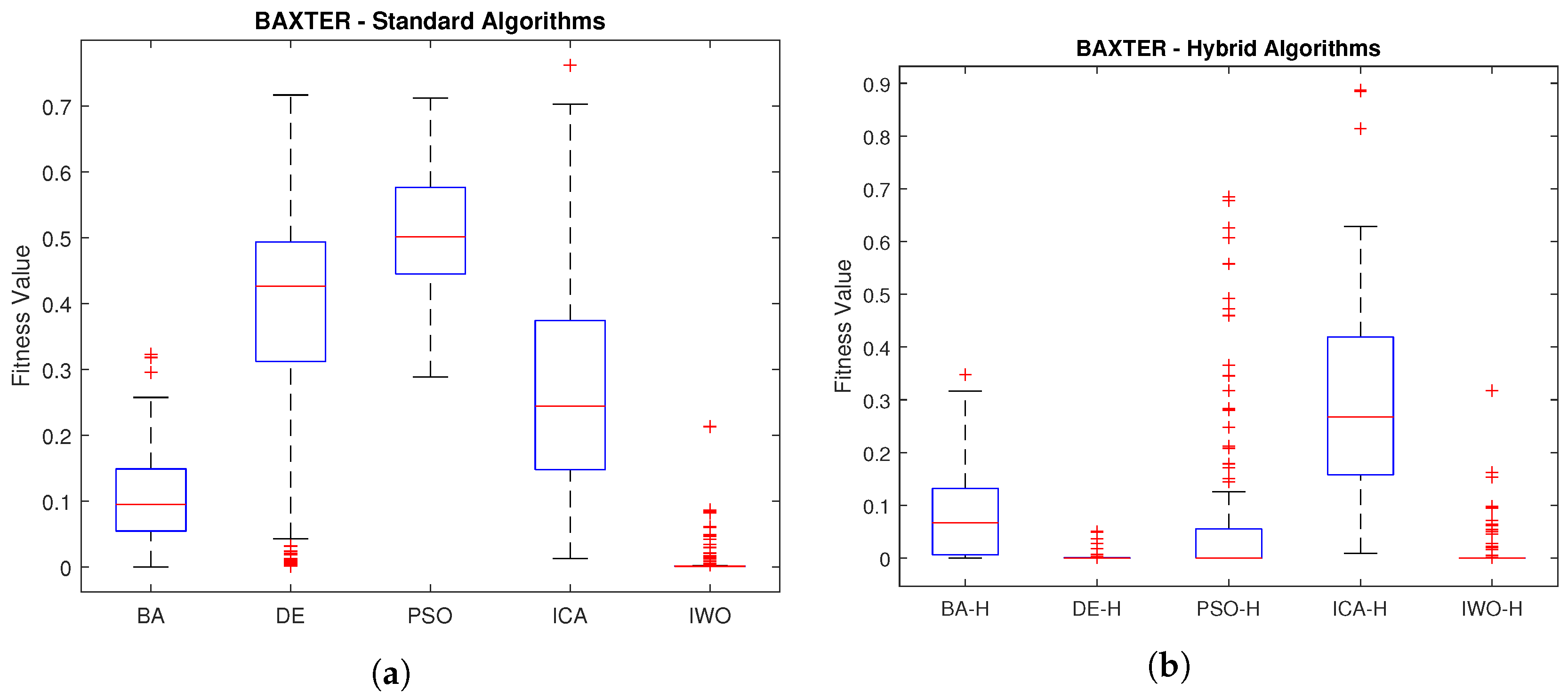
Figure 6 illustrates the simulation results for the 7 DOF Baxter robot. Figure 6a shows the data dispersion of standard algorithms, while Figure 6b demonstrates that the hybrid DE algorithm achieved the best result.

Table 6. Comparison of the statistical performance of standard and hybrid algorithms in solving the inverse kinematics of the Baxter robot. Bold text indicates better fitness values.

	BA	BA-H	DE	DE-H	PSO	PSO-H	ICA	ICA-H	IWO	IWO-H
mean	0.10814	0.08995	0.37702	2.2135$\times {\mathbf{10}}^{-3}$	0.50789	0.08282	0.29066	0.28297	0.01056	0.01515
std	0.07306	0.09374	0.19066	8.3733$\times {\mathbf{10}}^{-3}$	0.09158	0.16858	0.17908	0.18431	0.02845	0.04382
best	6.277 $\times {10}^{-5}$	2.023 $\times {10}^{-16}$	0.00146	2.0507 $\times {10}^{-15}$	0.28868	1.182 $\times {10}^{-16}$	0.00925	0.01281	0.00052	1.034$\times {\mathbf{10}}^{-16}$
worst	0.32282	0.34745	0.71676	0.05046	0.71212	0.68462	0.88735	0.7619	0.21314	0.31733

compares the statistical measures obtained by the algorithms in solving the inverse kinematics of the Baxter robot. Similar to the previous case, the hybrid DE algorithm (DE-H) exhibits the best performance.

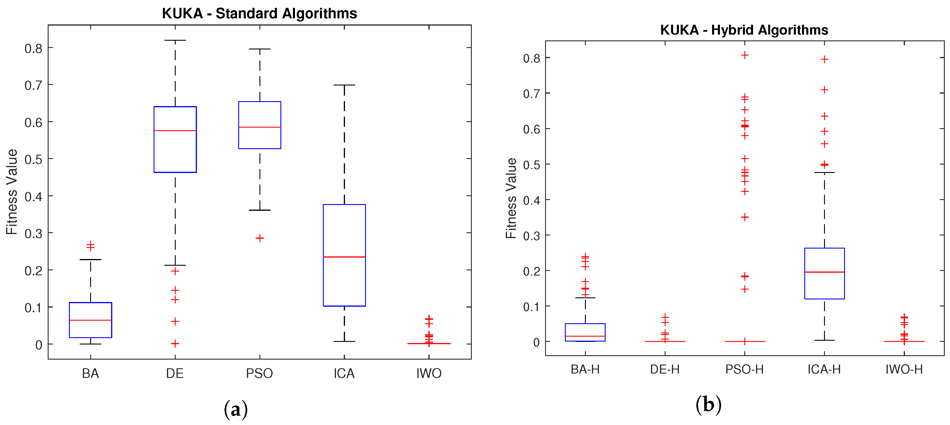
Finally, Figure 7 presents the simulation results of KUKA iiwa robot. Figure 7a displays a boxplot of the error obtained by the standard algorithms, while Figure 7b shows a boxplot of the performance of the hybrid algorithms. The distribution comparison indicates that hybrid algorithms perform better, with DE and IWO demonstrating similar performance.

Table 7. Comparison of the statistical performance of standard and hybrid algorithms in solving the inverse kinematics of the KUKA iiwa robot. Bold text indicates better fitness values.

	BA	BA-H	DE	DE-H	PSO	PSO-H	ICA	ICA-H	IWO	IWO-H
mean	0.070788	0.03839	0.54176	1.713$\times {\mathbf{10}}^{-3}$	0.58431	0.09882	0.24972	0.21884	3.777 $\times {10}^{-3}$	3.104 $\times {10}^{-3}$
std	0.06056	0.05618	0.14931	9.085$\times {\mathbf{10}}^{-3}$	0.10027	0.21386	0.17055	0.15758	0.01121	0.01208
best	2.514 $\times {10}^{-7}$	2.635 $\times {10}^{-16}$	0.00104	1.024 $\times {10}^{-16}$	0.28584	7.124$\times {\mathbf{10}}^{-17}$	0.00695	0.00343	0.00058	1.517 $\times {10}^{-16}$
worst	0.26805	0.23892	0.81966	0.06788	0.79564	0.80686	0.69871	0.79523	0.06801	0.06838

reveals that DE hybrid algorithm (DE-H) achieves the most significant improvement for the KUKA iiwa Robot.

5.2. Second Simulation Experiment

In this part of the simulations, an edge-case experiment is conducted to evaluate the proposed approach. To solve the inverse kinematics, a desired end-effector position is proposed within the workspace to ensure it is reachable. However, some desired positions cannot be achieved with certain orientations. Therefore, appropriate orientation selection is crucial. This issue makes the inverse kinematics problem challenging to solve.

In these edge cases, gains $k_t$ and $k_R$ in Equation (11) can be adjusted to give priority to minimize the error between the desired and the current end-effector position, rather than orientation errors.

The edge-case experiments involve defining a reachable desired position with an unreachable desired orientation for the Baxter robot. The proposed approach is run independently 100 times for the same pose, and the best fitness value is retained for statistical analysis to compare all considered algorithms. Additionally, position and orientation errors between the desired and current end-effector poses are analyzed (see Equation (11)).

The experimental setup is conducted as follows: gains are set to $k_t=1.5$ and $k_R=0.25$ to give priority to minimize the position error. Moreover, $G=300$, $N=30$, $\gamma =1000$, $C_R=0.9$, and $F=0.6$. Finally, the desired end-effector pose is defined as

$${\mathbf{T}}_d=\left[\begin{array}{cc}\hfill {\mathbf{R}}_d\hfill & {\mathbf{t}}_d\\ \hfill \mathbf{0}\hfill & 1\end{array}\right]=\left[\begin{array}{cccc}\hfill 0\hfill & 0& \hfill -1\hfill & 0.5\\ \hfill 0\hfill & -1& \hfill 0\hfill & 0.4\\ \hfill -1\hfill & 0& \hfill 0\hfill & 0.6\\ \hfill 0\hfill & 0& \hfill 0\hfill & 1\end{array}\right]$$

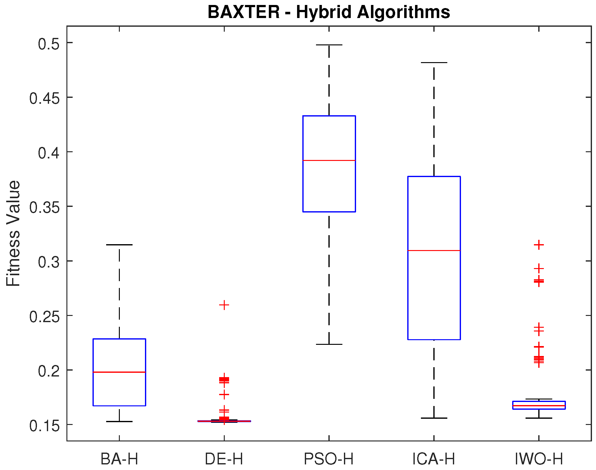
Figure 8 presents the statistical results of the best fitness value achieved by each algorithm. As shown, DE-H outperformed the others, demonstrating a smaller data distribution and lower fitness values. It is worth noting that the best fitness values are around 0.15 due to the significant orientation error. Consequently, position and orientation errors are now compared independently for statistical analysis.

Table 8. Statistical comparison of the performance of hybrid algorithms in solving the inverse kinematics of the Baxter robot with an unreachable desired end-effector orientation. Bold text indicates superior position error values.

	BA-H	DE-H	PSO-H	ICA-H	IWO-H
mean	0.00125	3.848$\times {\mathbf{10}}^{-4}$	0.09077	3.921 $\times {10}^{-3}$	0.011339
std	0.00761	0.00125	0.04460	0.00144	0.00541
best	3.809 $\times {10}^{-11}$	3.706 $\times {10}^{-6}$	0.01205	6.844$\times {\mathbf{10}}^{-16}$	0.00190
worst	0.07373	9.217$\times {\mathbf{10}}^{-3}$	0.21037	0.01013	0.02502

presents the position error results. The DE-H algorithm outperformed the others, achieving the lowest mean and standard deviation (std) values. Even the worst position error obtained by DE-H is better than the mean errors of BA-H, PSO-H, and IWO-H. Although the best position error is achieved by ICA-H, its performance is considered an outlier due to the larger data distribution observed in Figure 8.

In contrast to the position errors, the orientation errors reported in

Table 9. Statistical comparison of the performance of hybrid algorithms in solving the inverse kinematics of the Baxter robot with an unreachable desired end-effector orientation. Bold text indicates lower orientation error values.

	BA-H	DE-H	PSO-H	ICA-H	IWO-H
mean	0.80584	0.62786	0.99834	1.2006	0.64396
std	0.1702	0.05801	0.32869	0.35645	0.11902
best	0.61119	0.59024	0.37152	0.62033	0.54221
worst	1.2591	1.0353	1.8244	1.9267	1.1768

are significantly higher, as the desired orientation is considered unreachable.

As expected, DE-H reported lower mean, standard deviation (std), and worst-case orientation error values compared to those in reachable poses. Although the best orientation error was achieved by PSO-H, its data distribution, as shown in Figure 8, is considerably larger than that of DE-H.

We present another edge-case experiment involving four randomly selected unreachable desired positions, each with a corresponding reachable desired orientation, for the Baxter robot.

Table 10. Position and orientation error results of unreachable poses in Baxter robot.

Random Pose	Position Error	Orientation Error
1	0.47979	3.1913 $\times {10}^{-5}$
2	0.73254	9.575 $\times {10}^{-5}$
3	0.71156	3.0564 $\times {10}^{-4}$
4	0.94969	3.2291 $\times {10}^{-5}$

presents the position and orientation error results for each case, while Figure 9 illustrates the performance of the proposed approach in handling these unreachable poses. Coordinate frames in red represent the unreachable poses and coordinate frames in blue the achieved ones. Notice that all coordinate frames are adjusted with respect to orientation errors; however, position errors are not.

The results demonstrate that the proposed approach successfully solves the inverse kinematics problem by minimizing position errors, even when the desired orientation is unreachable.

5.3. Real-World Experimental Results

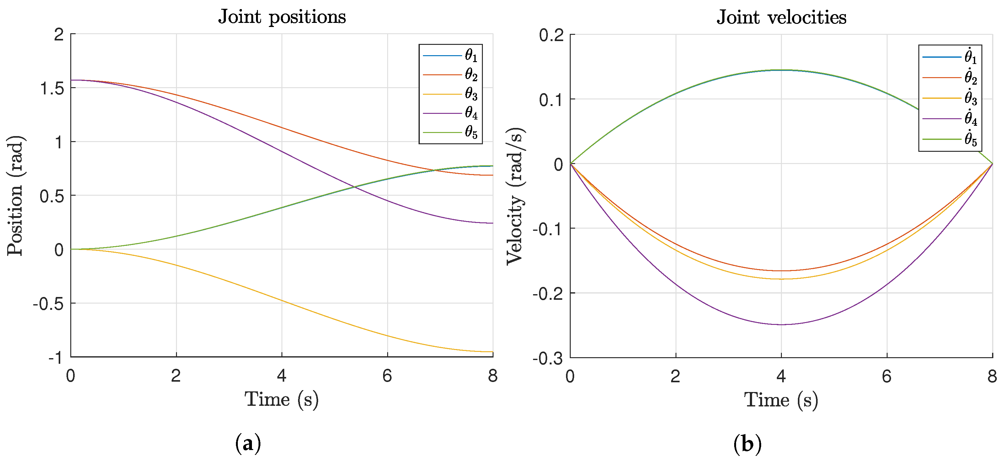
Real-world experiments were conducted to demonstrate the applicability of the proposed approach. The optimal joint configuration computed by this method can serve as a reference for point-to-point motion planning. For the experiments, a cubic polynomial trajectory was used to compute the joint motion from an initial joint position ${\mathbf{q}}_i$ to the joint reference ${\mathbf{q}}_r$ at a desired run time T.

The experimentation consists of two phases. First, the proposed approach solves the inverse kinematics for a desired end-effector pose to estimate a joint reference ${\mathbf{q}}_r$. Then, the manipulator robot follows a cubic polynomial trajectory based on the initial joint configuration ${\mathbf{q}}_i$ and a run time T.

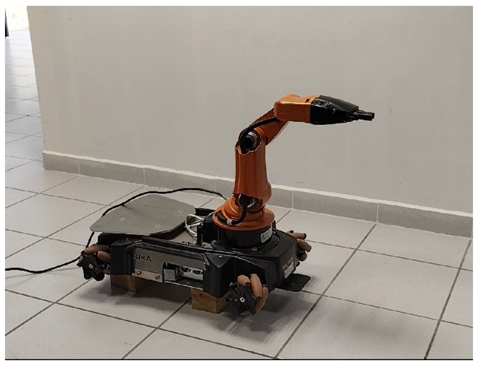
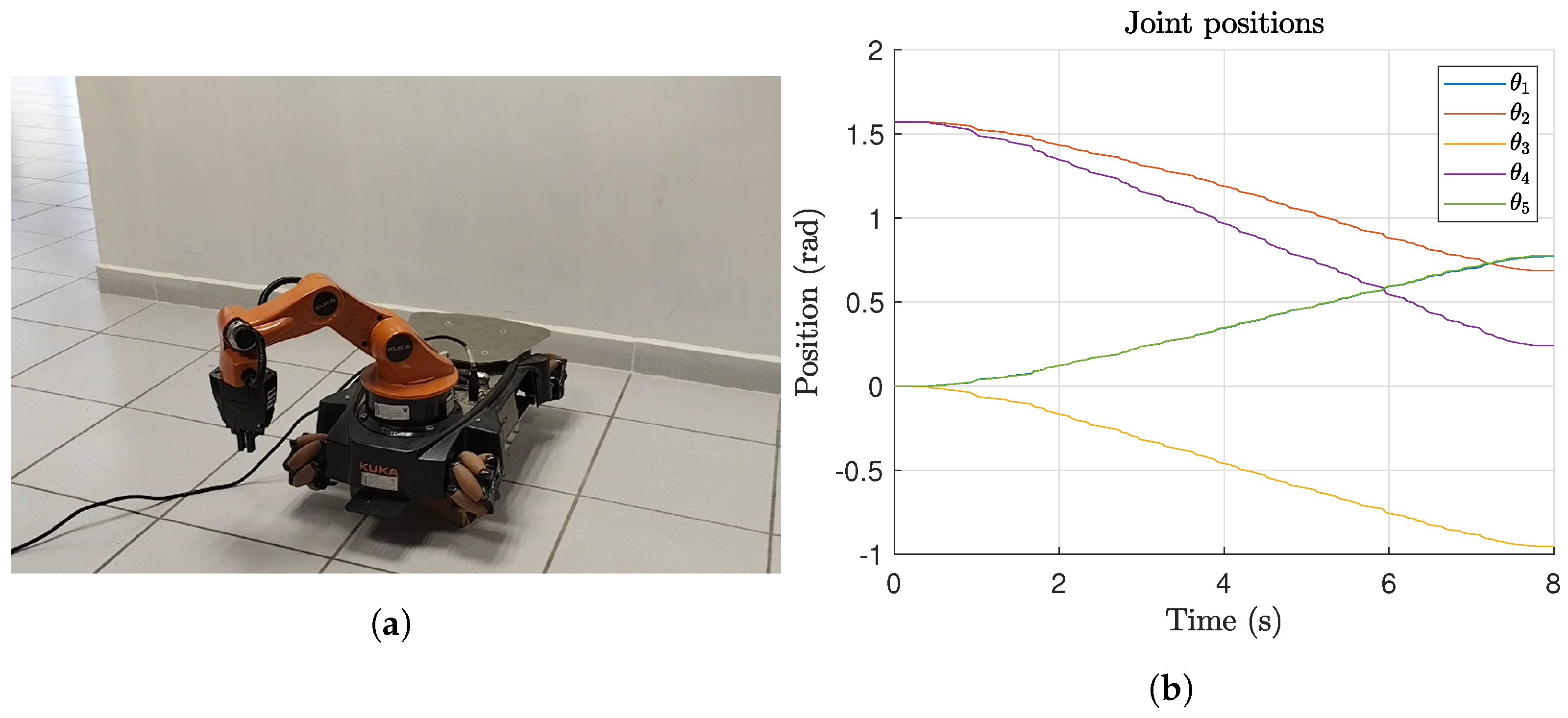
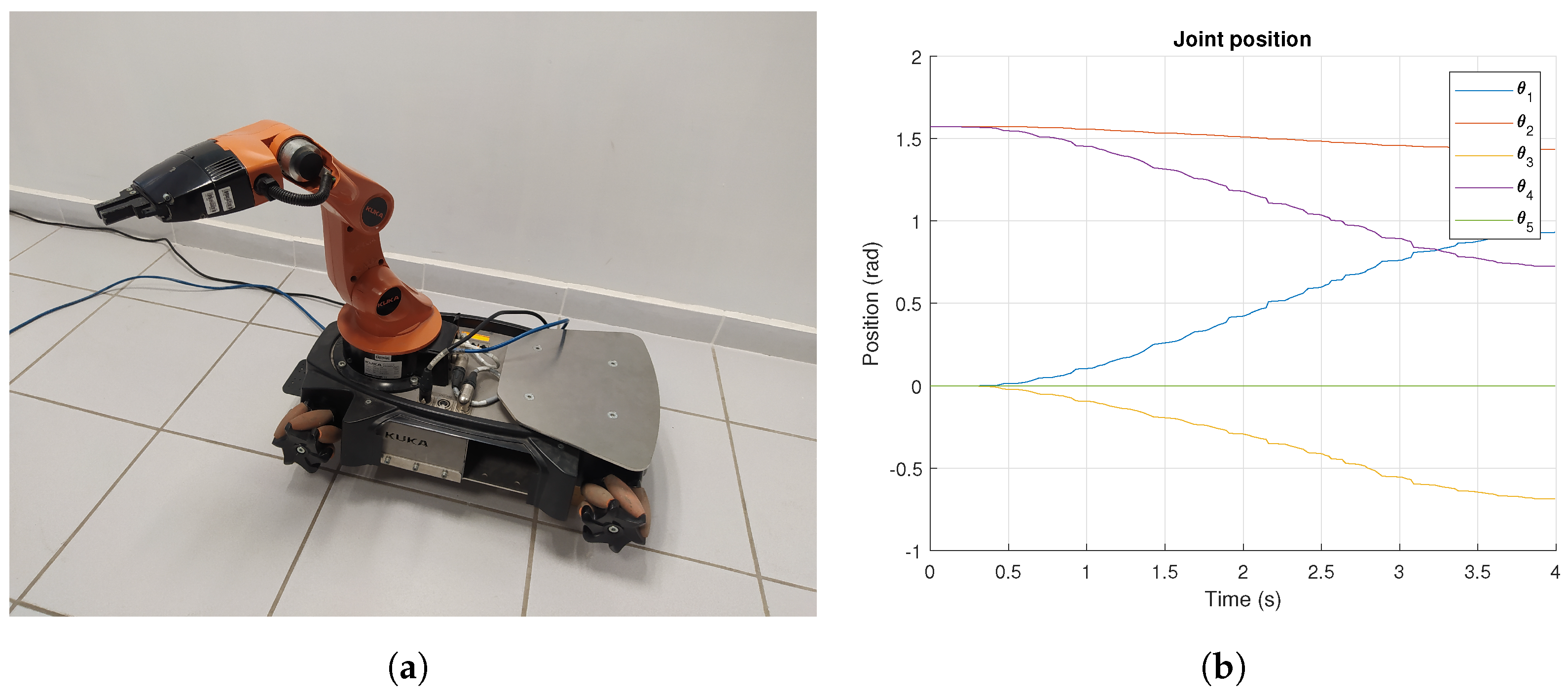
A 5 DOF KUKA YouBot was used for experimentation, as shown in Figure 10. The DH parameters are provided in

Table 11. DH parameters of KUKA YouBot manipulator.

Joint	a [m]	$\mathit{\alpha }$ [rad]	d [m]	$\mathbf{\Theta }$ [rad]
1	0.033	$\pi /2$	0.147	$q_1$
2	0.155	0	0	$q_2$
3	0.135	0	0	$q_3$
4	0	$\pi /2$	0	$q_4$
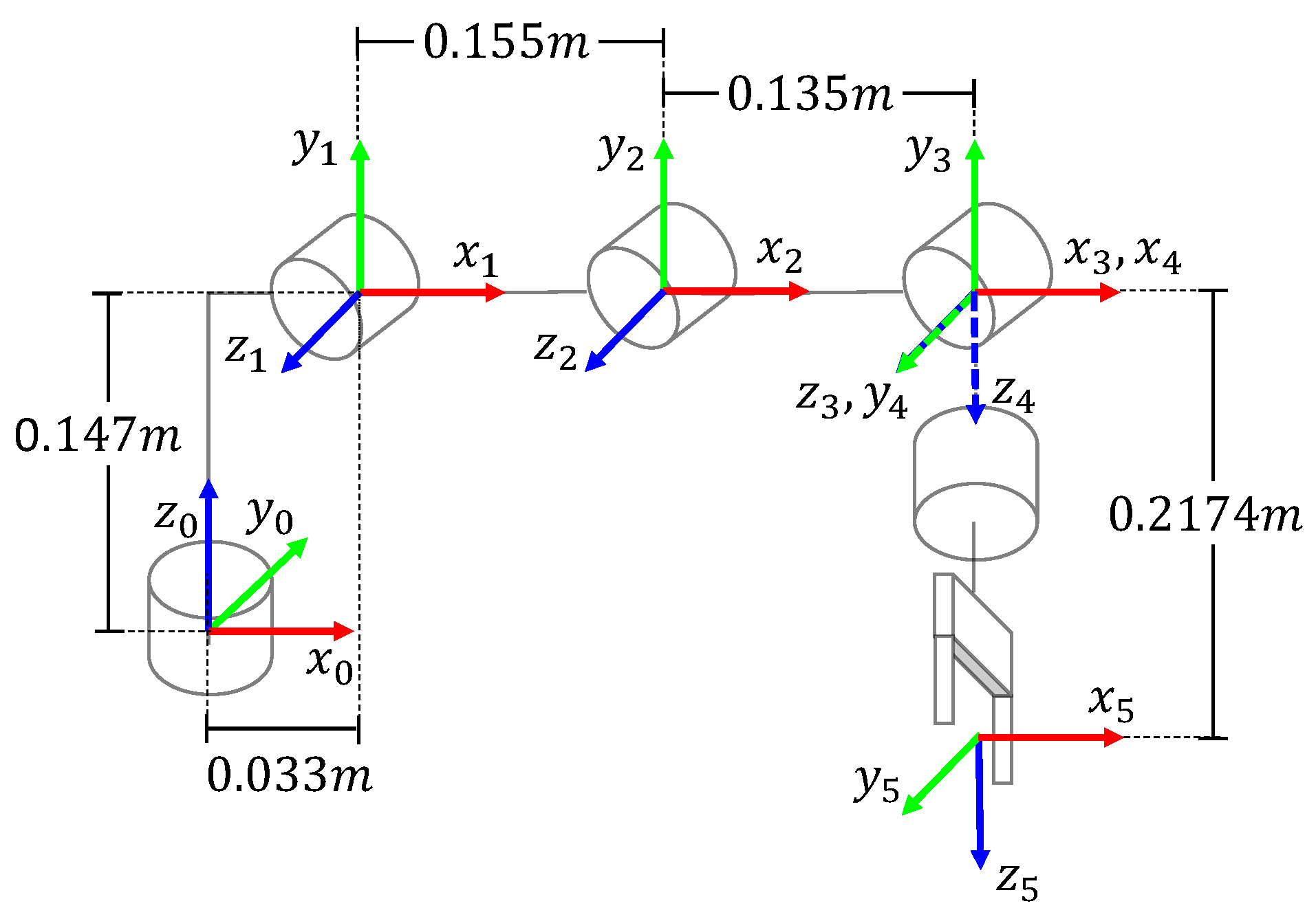
5	0	0	0.2174	$q_5$

and the coordinate frame assignment is presented in Figure 11. The proposed algorithm was implemented using Matlab and the ROS environment. ROS components on the KUKA YouBot provide an internal PID controller in the joint space, which is convenient for the considered trajectory planning. A point-to-point trajectory planning is performed on an external computer with Matlab and the ROS toolbox.

The lower and upper joint limits are defined as

$$\begin{array}{ccc}\hfill {\mathbf{q}}_l& =& {\left[\begin{array}{ccccc}-169& -65& -150& -102.5& -167.5\end{array}\right]}^T\hfill \\ \hfill {\mathbf{q}}_u& =& {\left[\begin{array}{ccccc}169& 90& 146& 102.5& 167.5\end{array}\right]}^T\hfill \end{array}$$

In Experiment 1, a run time of $T=8$ seconds is set, and the desired pose of the end-effector is specified as follows:

$${\mathbf{T}}_d=\left[\begin{array}{cc}\hfill {\mathbf{R}}_d\hfill & {\mathbf{t}}_d\\ \hfill \mathbf{0}\hfill & 1\end{array}\right]=\left[\begin{array}{cccc}\hfill 1& \hfill 0& \hfill 0& \hfill 0.2\\ \hfill 0& \hfill -1& \hfill 0& \hfill -0.2\\ \hfill 0& \hfill 0& \hfill 1& \hfill 0\\ \hfill 0& \hfill 0& \hfill 0& \hfill 1\end{array}\right]$$

(18)

The inverse kinematics solution obtained through the proposed approach is

$${\mathbf{q}}_r={\left[\begin{array}{ccccc}44.15& 39.31& -54.6& 13.57& 44.43\end{array}\right]}^T$$

The initial joint configuration is selected as

$${\mathbf{q}}_i={\left[\begin{array}{ccccc}0& 90& 0& 90& 0\end{array}\right]}^T$$

The joint position and velocities for the motion planning in Experiment 1 are presented in Figure 12. Additionally, Figure 13 illustrates the final joint configuration along with the joint motion results as measured by the encoders.

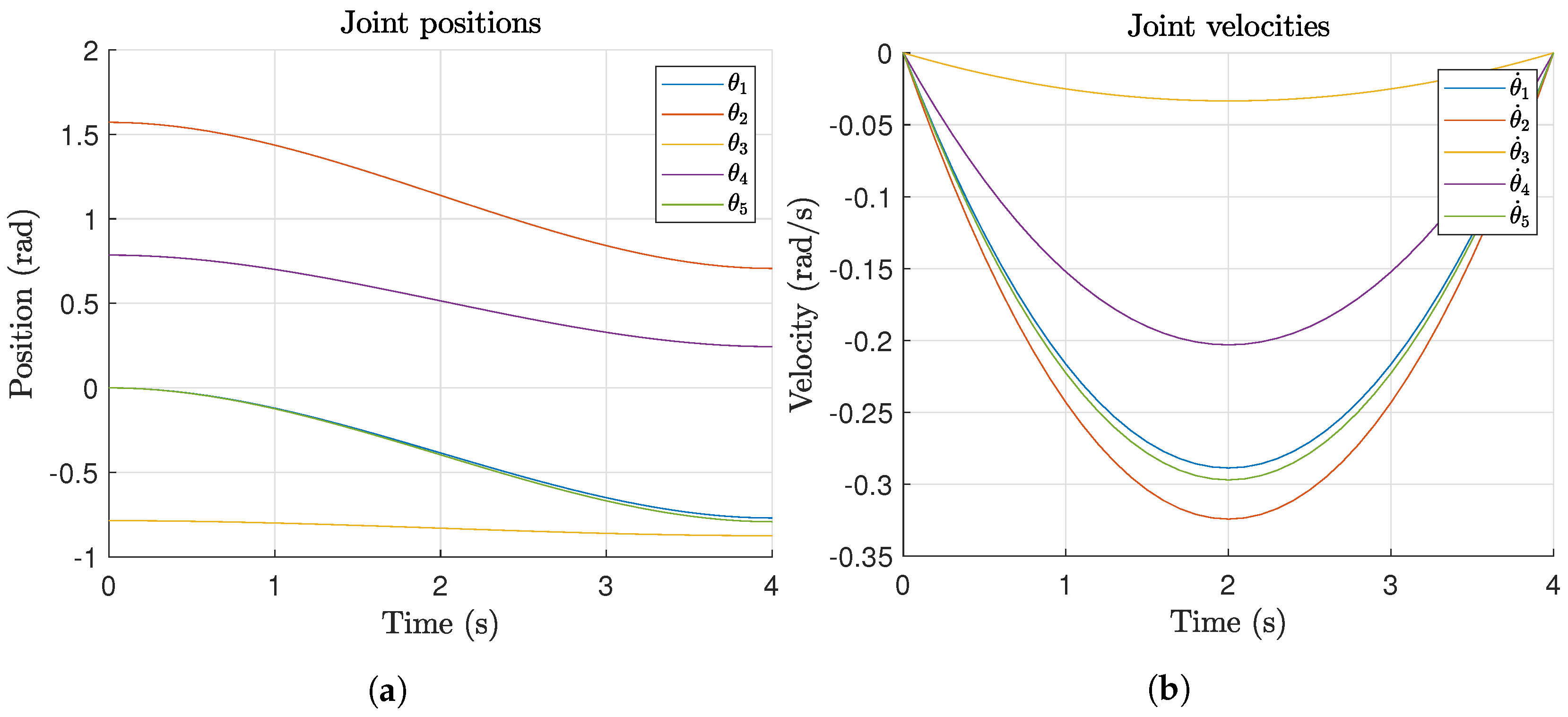
For Experiment 2, a run time of $T=4$ seconds is set, and the desired pose of the end-effector is defined as

$${\mathbf{T}}_d=\left[\begin{array}{cc}\hfill {\mathbf{R}}_d\hfill & {\mathbf{t}}_d\\ \hfill \mathbf{0}\hfill & 1\end{array}\right]=\left[\begin{array}{cccc}\hfill 1& \hfill 0& \hfill 0& \hfill 0.2\\ \hfill 0& \hfill -1& \hfill 0& \hfill 0.2\\ \hfill 0& \hfill 0& \hfill 1& \hfill 0\\ \hfill 0& \hfill 0& \hfill 0& \hfill 1\end{array}\right]$$

The inverse kinematics solution for Experiment 2, obtained through the proposed approach, is

$${\mathbf{q}}_r={\left[\begin{array}{ccccc}-44.10& 40.46& -50.10& 13.97& -45.37\end{array}\right]}^T$$

and the considered initial joint configuration for this test is

$${\mathbf{q}}_i={\left[\begin{array}{ccccc}0& 90& -45& 45& 0\end{array}\right]}^T$$

The joint position and velocities of the motion planning for Experiment 2 are presented in Figure 14. Additionally, Figure 15 illustrates the final joint configuration along with the joint motion results measured by the encoders.

As observed in Figure 13b and Figure 15b, the internal controller follows the given joint references given in Figure 12 and Figure 14, respectively. This indicates that the manipulator reached the optimal joint configurations computed by the proposed approach. Furthermore, Figure 13 and Figure 15 illustrate the real-world applicability of the proposed approach; the computed joint configurations are physically reachable.

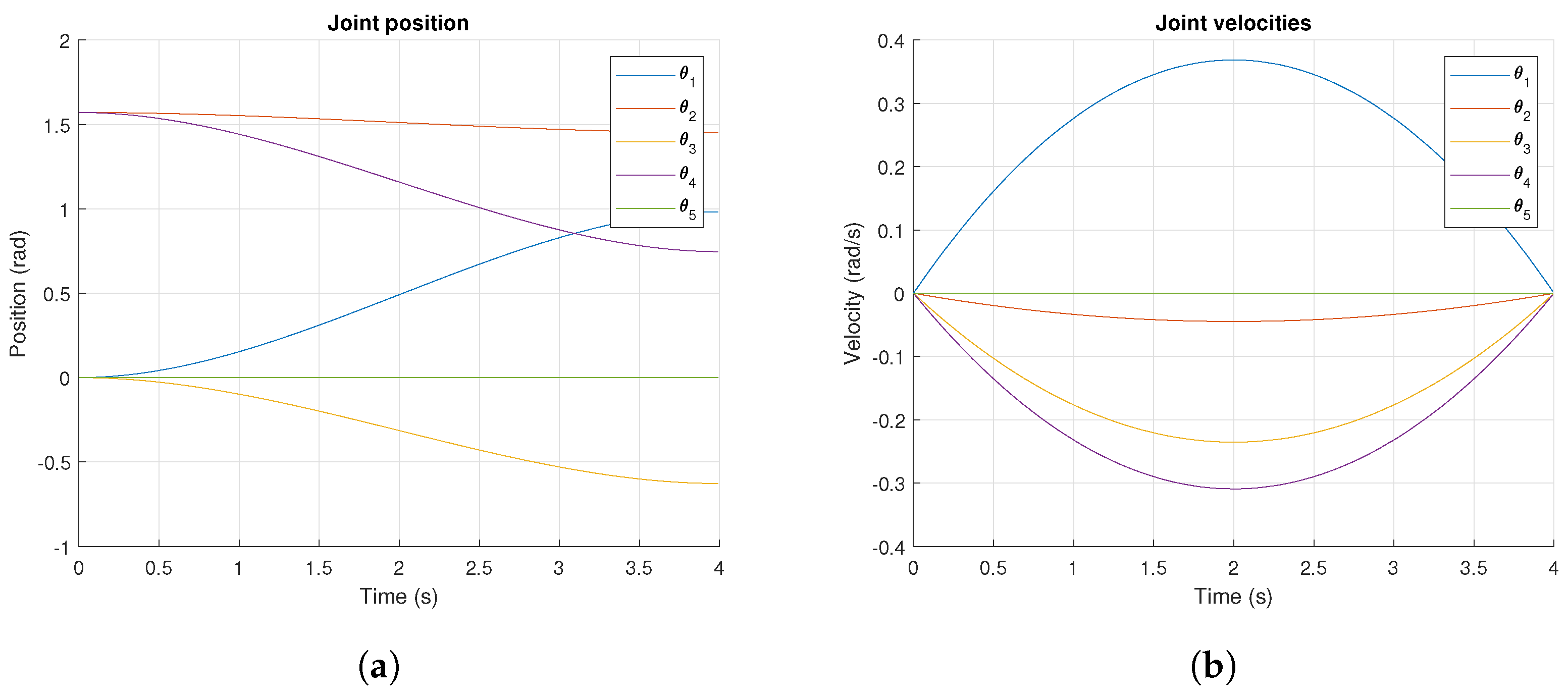
For Experiment 3, a runtime of T = 4 s is set. In this case, a desired end-effector pose is defined with a reachable position but an unreachable orientation. The desired pose is specified as follows:

$${\mathbf{T}}_d=\left[\begin{array}{cc}\hfill {\mathbf{R}}_d\hfill & {\mathbf{t}}_d\\ \hfill \mathbf{0}\hfill & 1\end{array}\right]=\left[\begin{array}{cccc}\hfill 0& \hfill 0& \hfill 1& \hfill 0.2\\ \hfill 0& \hfill -1& \hfill 0& \hfill 0.3\\ \hfill 1& \hfill 0& \hfill 0& \hfill 0.4\\ \hfill 0& \hfill 0& \hfill 0& \hfill 1\end{array}\right]$$

The inverse kinematics solution for experiment 3 is

$${\mathbf{q}}_r={\left[\begin{array}{ccccc}56.31& 83.19& -35.95& 42.76& 0.0028\end{array}\right]}^T$$

The initial joint configuration considered for the polynomial trajectory is as follows:

$${\mathbf{q}}_i={\left[\begin{array}{ccccc}0& 90& 0& 90& 0\end{array}\right]}^T$$

The joint positions and velocities for the motion planning are shown in Figure 16. Additionally, Figure 17 presents the final joint configuration along with the joint motion results measured by the encoders.

The achieved end-effector pose is

$${}^0\mathbf{T}_n=\left[\begin{array}{cccc}\hfill 0& \hfill 0.832& \hfill 0.554& \hfill 0.2\\ \hfill 0& \hfill -0.554& \hfill 0.832& \hfill 0.3\\ \hfill 1& \hfill 0& \hfill 0& \hfill 0.4\\ \hfill 0& \hfill 0& \hfill 0& \hfill 1\end{array}\right]$$

As can be seen, the desired position is reached. The desired and current positions are practically the same. However, the desired and current orientations are only approximately aligned. As expected, the proposed approach prioritizes minimizing position errors over orientation errors, given that the desired orientation is not reachable. It is worth noting that the implementation in real-world experiments further demonstrates that the inverse kinematics solutions are physically feasible.

The proposed algorithm was executed on a computer with an Intel i7 processor and 16 GB of RAM. The inverse kinematics estimation took less than one second for each tested point. If further speed is required, the performance of metaheuristic algorithms can be enhanced using parallel architectures and dedicated hardware, such as NVIDIA CUDA.

6. Discussion

The proposed approach was applied in three simulation experiments involving the Puma-560, Baxter, and KUKA iiwa robots. The inverse kinematics were successfully solved in each case, demonstrating the applicability of the system across different configurations. Among the tested algorithms, differential evolution (DE) consistently outperformed BA, PSO, and ICA. While the performance of DE and IWO exhibited similar performance across experiments, DE reported the lowest dispersion of the data.

When comparing the experimental results with and without hybridization, a significant improvement in the solution of the inverse kinematics is evident across all algorithms. The Jacobian step enhances the exploitation capabilities of the algorithm; algorithms like PSO, ICA, and BA exhibit stagnation, which indicates weak exploration capabilities, whereas DE and IWA demonstrate a strong exploration performance.

DE-H reported better fitness value results in all tests, achieving the lowest mean and standard deviation (std) values. This indicates that DE-H achieved the smallest error in both position and orientation with precision, along with the smallest data distribution, reflecting more consistent results. In contrast, ICA and PSO performed poorly in all tests, achieving the worst results in terms of mean and std values. Additionally, the performance of IWO-H was very similar to DE-H. However, DE-H outperformed all the other algorithms by achieving lower mean and std values.

The evaluation of the standard deviation ($5.8348 \times {10}^{-3}$) indicates that the method achieves sufficient precision in both position and orientation, making it suitable for applications such as medical procedures, where fine adjustments are critical.

The proposed approach was also applied in real-world experimentation, where the KUKA YouBot robot was considered as a case study. The application on the real robot demonstrates that the inverse kinematics results are acceptable, confirming that the constrained problem is solved despite the DE algorithm not being specifically designed for constrained problems.

A drawback of the conventional Jacobian pseudoinverse is that the inversion of J cannot always be guaranteed. Singular configurations cause J to become rank deficient, leading to system instability. In this work, a Jacobian pseudoinverse step is used to generate a candidate solution. In the presence of singularities, unfeasible solutions are avoided in the Jacobian pseudoinverse operation, as only improved joint solutions replace the current ones. This mechanism effectively prevents singularities.

Future work will focus on solving inverse kinematics for a mobile manipulator [16], incorporating the Jacobian step for fine-tuning. Additionally, we aim to extend the use of inverse kinematics to trajectory tracking and address grasping problems on platforms equipped with dual manipulators [35,36].

7. Conclusions

The hybrid metaheuristic algorithm approach proposed in this paper has demonstrated its applicability across different robotic manipulators by successfully solving inverse kinematics in two simulated experiments with six and seven degrees of freedom, as well as in an experiment with a real robot with five degrees of freedom.

Among the algorithms tested in this research, DE and IWO exhibited similar performance across the experiments. However, DE achieved the lowest scatter in the data, effectively solving both position and orientation with constraints, even though the algorithm was not designed to work with constraints.

The inclusion of the Jacobian matrix steps shows a significant improvement in the exploitation capabilities of the algorithms, However, algorithms with inherently poor exploration characteristics showed only marginal improvement.

Future work applying the methods proposed in this study promises favorable results for more complex problems, such as dual-arm systems and mobile manipulators. This work considers solving the inverse kinematics for manipulators with open kinematic chains. However, it is appealing to extend this work to solve the inverse kinematics of closed kinematics such as parallel manipulators.