Abstract
In this manuscript, we carry out a study on the generalization of a known family of multipoint scalar iterative processes for approximating the solutions of nonlinear systems. The convergence analysis of the proposed class under various smooth conditions is provided. We also study the stability of this family, analyzing the fixed and critical points of the rational operator resulting from applying the family on low-degree polynomials, as well as the basins of attraction and the orbits (periodic or not) that these points produce. This dynamical study also allows us to observe which members of the family are more stable and which have chaotic behavior. Graphical analyses of dynamical planes, parameter line and bifurcation planes are also studied. Numerical tests are performed on different nonlinear systems for checking the theoretical results and to compare the proposed schemes with other known ones.
1. Introduction
Many papers deal with methods and families of iterative schemes to approximate the solution of nonlinear equations , with as a function defined in an open interval I. Each of them has a different behavior due to their order of convergence, stability and efficiency. Of the existing methods in the literature, in the present manuscript, we focus on the family of iterative processes (ACTV) for approximating the solutions of nonlinear equations, proposed by Artidiello et al. in [1]. This family was constructed adding a Newton step to Ostrowski’s scheme, and using a divided difference operator. Then, the family has a three-step iterative expression with an arbitrary complex parameter . Moreover, its order of convergence is at least six. Its iterative expression is
where
The divided difference operator is defined as
By using tools of complex dynamics, the stability of this family was studied by Moscoso [2], where it was observed that there is good dynamic behavior in the case of . In Section 2, we present the multidimensional extension of family (1) and prove its convergence order.
In the stability analysis (Section 3), we determine whether the fixed points of the associated rational operator are of an attracting, repulsing or saddle point nature; on the other hand, we search for which values of the parameter-free critical points may appear. In the bifurcation analysis of free critical points (Section 4), we calculate the parameter lines, which we generate from the mentioned free critical points, then we generate the bifurcation planes for specific intervals of parameter , and as a consequence of these studies, we generate the dynamical planes for members of the family with stable and unstable behavior. In Section 5, some numerical problems are considered to confirm the theoretical results. The proposed schemes for different values of parameter are considered and compared with Newton’s method and some known sixth-order techniques, namely , , , , , , introduced by Cordero et al. in [3], Cordero et al. in [4], Behl et al. in [5], Capdevila et al. in [6], and Xiao and Yin et al. in [7].
The iterative expressions of these methods for solving a nonlinear systems , are shown below. Newton’s scheme is the most known iterative algorithm
where denotes the Jacobian matrix associated to F.
The following sixth-order iterative scheme (see [3]) is named . It uses three evaluations of F and two of , per iteration:
The following scheme, introduced in [4], is a modified Newton–Jarratt composition with sixth-order convergence and evaluates twice F and , per iteration. It is denoted by :
Algorithm (5) was constructed by Behl et al. in [5] and it is denoted by .
where and is a parameter. This is a class of iterative processes that achieves convergence order six with twice F evaluations and , per iteration. For our comparison, we will use two versions of method , one of them with and the other one with .
Capdevila et al. in [6] introduced the following class of iterative methods that we call . The elements of this family have an order of convergence of six and they need three evaluations of function F, one of the the Jacobian matrix and a divided difference per iteration:
where is free and . For the numerical results, we will take and .
Introduced also by Capdevila et al. in [6], we work with the following scheme, denoted , with the same order of convergence and the same number of functional evaluations per iteration as :
In this case, we take .
Finally, we use the method called introduced by Xiao and Yin in [7]. In this case, we need twice F evaluations and on , and , , respectively, per iteration.
Multidimensional Real Dynamics Concepts
Discrete dynamics is a very useful tool to study the stability of iterative schemes for solving nonlinear systems. An exhaustive description of this tool can be found in the book [8]. A resource used for the stability analysis of iterative schemes for solving nonlinear systems is to analyze the dynamical behavior of the vectorial rational operator obtained to apply the iterative expression on low degree polynomial systems. This technique generally uses quadratic or cubic polynomials [9].
When we have scalar iterative processes, the tools to be used are of real or complex discrete dynamics. However, here, we handle a family of vectorial iterative methods, so real multidimensional dynamics must be used to analyze its stability, see [6]. We proceed by taking a system of quadratic polynomials on which we will apply our method in order to obtain the associated multidimensional rational operator and perform the analysis of the fixed and critical points in order to select members of the family with good stability.
Some concepts used in this study are presented, see for instance [10].
Let be the operator obtained from the iterative scheme on a polynomial system . The set of successive images of through is called the orbit of . is a fixed point of G if . Of course, the roots of are a fixed point of G, but there may be fixed points of G that are not solutions of system . We refer them as strange fixed points. A point x that satisfies and , for and is called a periodic point, of period k. For classifying the stability of fixed or periodic points, we use the following result.
Theorem 1
([8], pg. 558). Let be of type . Assuming that is a periodic k-point, . If are the eigenvalues of , we have the following:
- (a)
- If all eigenvalues verify that , then is an attracting point.
- (b)
- If an eigenvalue is such that , then is unstable, that is, repulsor or saddle.
- (c)
- If all eigenvalues verify that , then is a repulsive point.
The set of preimages of any order of an attracting fixed point of the multidimensional rational function G, ,
is the basin of attraction of , .
The solutions of are called the critical point of operator G. The critical points different of the roots of are called a free critical point. The critical points are important for our analysis because of the following result from Julia and Fatou (see [11,12,13]).
Theorem 2
(Julia and Fatou). Let G be a rational function. The immediate basin of attraction of a periodic (or fixed) attractor point contains at least one critical point.
2. Family ACTV for Nonlinear Systems
Taking into account the iterative expression of family (1), we can extend, in a natural way, this expression for solving nonlinear systems . We change scalar by vectorial and by the divided difference operator . The resulting expression is
where is the identity matrix.
Mapping such that
is the divided difference operator of F on (see [14]).
The proof of the main result is based on the Genochi–Hermite formula (see [14]),
By developing in Taylor series around x, we obtain
Denoting by , where is a zero of , and assuming that is invertible, we obtain
where . Replacing these expressions in the Genocchi–Hermite formula and denoting the second point of the divided difference by and the error of y by , we obtain
Particularly, if y is the Newton approximation, i.e., , we obtain
Convergence Analysis
Theorem 3.
Being differentiable enough in an open convex neighborhood Ω of ξ, root of . Consider a seed close enough to the solution ξ and that is continuous and invertible in ξ. Then, (9) has a local convergence of order six, for all , with the error equation
being .
Proof.
From
We perform the Taylor series of and around ,
We suppose that the Jacobian matrix is nonsingular and calculate the Taylor expansion of as follows:
where are unknowns such that
Taking into account , the expansion of the error at the first step of family (1) is
For , we calculate up to order six using the Genochi–Hermite formula seen in (10), obtaining
Now, we obtain the expansion of ,
To obtain the error equation of the third step, we need the calculation of and since the other elements were previously obtained. Following a process similar to that seen in (17) and developing only to order two, we have that
For the calculation of , we are only interested in the terms up to order six, so applying what we see in formula (18), we obtain
The resulting error equation for the family of methods (9) is
□
Once the convergence order of the proposed class of the iterative method is proven, we undertake a complexity analysis, taking into account the cost of solving the linear systems and the rest of the computational effort, not only of the proposed class but also of Newton’s and those schemes presented in the Introduction, with the same order six. In order to calculate it, let us remark that the computational cost (in terms of products/quotients) of solving a linear system of size is
but if another linear system is solved with the same coefficient matrix, then the cost increases only in operations. Moreover, a matrix–vector product corresponds to operations. From these bases, the computational effort of each scheme is presented in Table 1. As the ACTV class depends on parameter , we consider , as this value eliminates one of the terms in the iterative expression, reducing the complexity.

Table 1.
Computational cost (products/quotients) of proposed and comparison methods.
Observing the data in Table 1, there seems to be a great difference among Newton’s and sixth-order methods, with , and being the most costly, in this order. Our proposed scheme ACTV for , stays in the middle values of the table. However, this must be seen in contrast with the order of convergence p of each scheme. With this point of view, the comparison among the methods is more clear.
With the information provided by Table 1, we represent in Figure 1 and Figure 2 the performance of the efficiency index of each method, where p is the order of the corresponding scheme. This index was introduced by Traub in [15], in order to classify the procedures by their computational complexity.
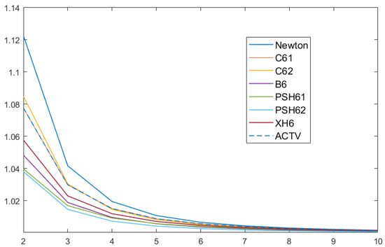
Figure 1.
Efficiency index IO for systems of size to .
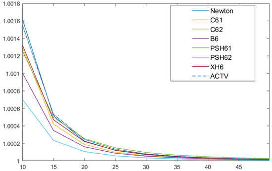
Figure 2.
Efficiency index IO for systems of size to .
In Figure 1, we observe that the best scheme is that of Newton, being that our proposed procedure (dashed line in the figure) is third in efficiency. This situation changes for bigger sizes of the system (see Figure 2), as ACTV for achieves the second best place, very close to Newton’s, improving the rest of schemes of the same order of convergence. Our concern now is the following: is it possible to find some values of the parameter such that this performance is held or even improved? The improvement can be in terms of the wideness of the set of converging initial estimations. This is the reason why we analyze the stability of the class of iterative methods.
3. Stability Analysis
Let us consider a polynomial system of n variables where and we denote by the associated rational function. From now on, we denote by the vectorial function obtained when class (9) is applied on . As is uncoupled, all functions are analogous, with the difference of the index . Their expressions are
where,
There are values of for which the operator coordinates are simplified; we show the particular case when .
By determining and analyzing the corresponding fixed points of the operator, we present a synthesis of the most relevant results.
Theorem 4.
Roots of are the components of superattracting fixed points of associated to the class of iterative methods (9). The same happens with the roots of depending on α:
- (a)
- If or , there are two real roots of , denoted by . Fixed points where , are repulsive points. However, if any of , , then they are saddle points.
- (b)
- has no strange fixed points for .
Proof.
To calculate the fixed points of , we solve ,
for , that is, and roots of , provided that .
At most, two of the roots of are not complex, depending on . The qualitative performance of is deduced from the eigenvalues of evaluated at the fixed points. Due to the nature of the polynomial system, these eigenvalues coincide with the coordinate function of the rational operator:
We calculate the absolute values of these eigenvalues only where fixed points are real; it is clear that those fixed points are super attracting.
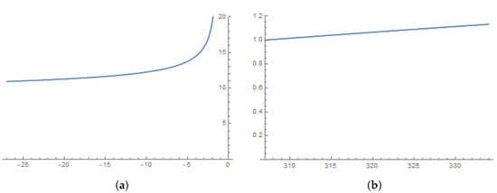
We proceed to plot some of the eigenvalues; if , the eigenvalues of at any strange fixed point are named saddle points when their combinations have some component +1,-1 and the combinations of real roots coming from are named repulsors because all eigenvalues are greater than 1 (see Figure 3a); if , a similar behavior is observed (see Figure 3b). □

Figure 3.
Eigenvalues associated to the fixed points. (a) . (b) .
Once the existence and stability of strange fixed points of is studied, our aim is to show if there exist any other attracting behavior different from the fixed points.
4. Bifurcation Analysis of Free Critical Points
In the following result, we summarize the most relevant results about critical points.
Theorem 5.
has as free critical points
make null the entries of the Jacobian matrix, for , being that is,
- (a)
- If , there not exist free critical points.
- (b)
- If , then two real roots of polynomial are components of the free critical point.
Proof.
The not null components of are
Then, the real roots of are free critical points, provided that they are not null. □
4.1. Parameter Line and Bifurcation Plane
Now, we use a graphical tool that helps us to identify for which values of parameters there might be convergence to roots, divergence or any other performance. Real parametric lines, for , are presented in Figure 4 and Figure 5 (see Theorem 5). In these figures, a different free critical point is employed as a seed of each member of the class, using and to ensure the existence of real critical points.

Figure 4.
Parameter line of in . (a) . (b) .
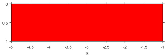
Figure 5.
Parameter line of in .
To generate them, a mesh of points is made in for the first figure and for the next. We use in Figure 4a to increase the interval where is defined and in Figure 4a and Figure 5, allowing a better visualization. So, the color corresponding to each value of is red if the corresponding critical point converges to one of the roots of the polynomial system, blue in the case of divergence, and black in other cases (chaos or periodic orbits). In addition, we use 500 as the limit of iterations and tolerance .
The global performance of each pair of free critical points is similar, so only is shown in Figure 4. In Figure 4a, only a small black region shows non-convergence to the roots (red color). Now we show the parameter line for .
In the line shown in Figure 5 it is observed that the zone shows global convergence to the roots. Therefore, it is a good area for choosing .
The concept of bifurcation is important in nonlinear systems since it allows us to study the behavior of the solutions of a family of iterative methods. In reference to dynamical systems, a bifurcation occurs when a small variation in the values of the system parameters (bifurcation parameters) causes a qualitative or topological change in the behavior of the system. Feigenbaum or bifurcation diagrams appear to analyze the changes of each class of methods on by using each critical point of the function as a seed and observing its performance for different ranges of . By using a mesh with 4000 subintervals in each axis and after 1000 iterations, different behaviors can be observed.
Figure 6 shows the bifurcation diagrams in the black area of the parameter line Figure 4b, specifically when . In Figure 6a, a general convergence to one of the roots appears. However, a quadruple-period orbit can be found in a small interval around . It includes not only periodic but also chaotic behavior (strange attractors, blue regions).
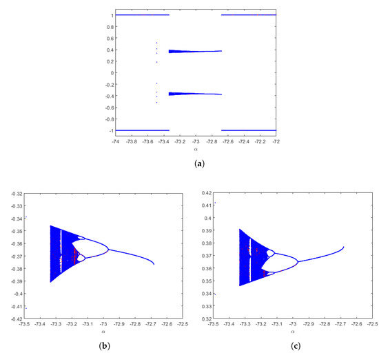
Figure 6.
Feigenbaum diagrams of , for , from different critical points. (a) and . (b) a detail. (c) a detail.
To obtain the strange attractors, we plot in Figure 7 and Figure 8 the orbit of 1000 initial guesses close to point in the -space by iterating . The value of the parameter used is , laying in the blue region. For each seed, the first 500 iterations are ignored; meanwhile, the following 400 appear in blue and the last 100 in magenta color. We see in Figure 7 and Figure 8 that a parabolic fixed point bifurcates in periodic orbits with increasing periods, and therefore falls in a dense orbit (chaotic behavior) in a small area of space.
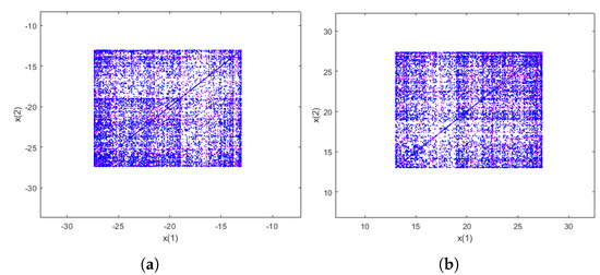
Figure 7.
Strange attractors of for in blue quadruple-period cascade. (a) . (b) .
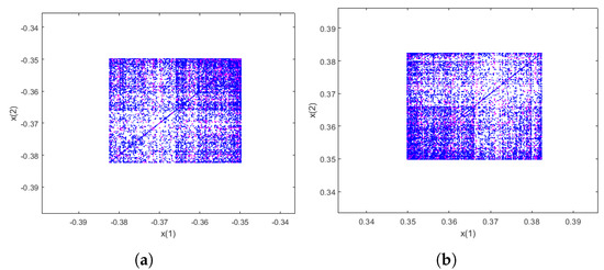
Figure 8.
Details Strange attractors of . (a) a detail. (b) a detail.
For values of , the bifurcation diagrams can be observed in Figure 9. It is related to the black region of Figure 4b. In addition, it can be observed a general convergence to one of the roots, but a sixth-order periodic orbit appears in a small interval around . It includes chaotic behavior (blue regions) beside periodic performance. Strange attractors can be found in them. To represent it, we plot in Figure 10 the -space the orbit of by , for , laying in the blue region.
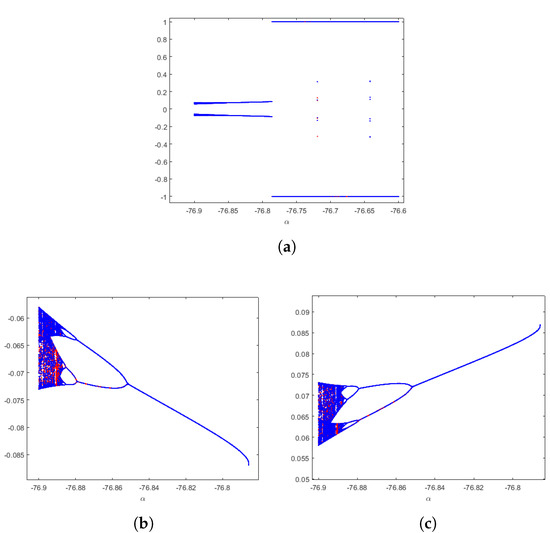
Figure 9.
Feigenbaum diagrams of , for , from different critical points. (a) and . (b) a detail. (c) a detail.
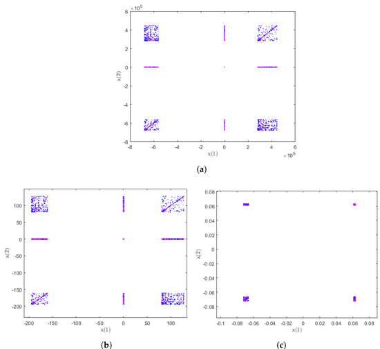
Figure 10.
Strange attractors of for in blue quadruple-period cascade. (a) . (b) a detail. (c) into the detail.
4.2. Dynamical Planes
The tool with which we can graphically visualize most of the information obtained is the dynamical planes; in these, we represent the basins of attraction of the attracting fixed points for several values of parameter . The above mentioned can only be done when the nonlinear system has a dimension of 2, although the results of the dynamical analysis are valid for any dimension.
To calculate the dynamical planes for the systems, a grid of points is defined in the real plane, and each point is used as an initial estimate of the iterative method for a fixed . If the iterative method converges to some zero of the polynomial from a particular point of the grid, then it is assigned a certain color; in particular, if it only converges to the roots of , the predominant colors are orange if it converges to , blue if it converges to , green if it converges to and brown if it converges to . If, as an initial estimate, a point has not converged to any root of the polynomial in 100 iterations at most, it is assigned as black. The colors in certain basins are darker or not, indicating that the orbit in certain initial estimate will converge to the fixed point of the basin with greater or fewer iterations, with the lighter colors causing fewer iterations.
For with stable behavior, we elaborate our graph that has a grid with 500 × 500 points, with 100 as the maximum number of iterations and limit of [−5, 5] for both axes (see Figure 11), for values of in unstable regions the interval is [−40, 40] in both axes in Figure 12 and [−30, 30] in Figure 13. Periodic orbits are also observed in Figure 13.
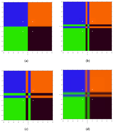
Figure 11.
Dynamical planes for some stable values of parameter . (a) . (b) . (c) . (d) .
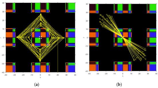
Figure 12.
Unstable dynamical planes of on . (a) . (b) .
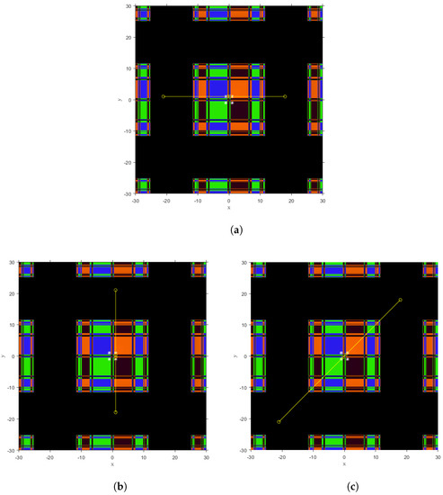
Figure 13.
Periodic orbits for parameter for different initial values. (a) . (b) . (c) .
In Figure 11a, we see four basins of attraction that correspond to the roots of polynomial system, with a very stable behavior. However, each basin of attraction has more than one connected component for and , as can be seen in Figure 11b,c, respectively. This performance increases for lower values of close to the instability zones seen in the parameter lines Figure 4b, as seen in Figure 11d.
In Figure 12, we can see a chaotic behavior (chaos) when we take initial estimations in the black zones, producing orbits with random behavior that do not lead to the expected solution. Finally, in Figure 13, the phase space for is plotted. In them, the following 3-period orbits are painted in yellow:
- ,
- ,
- ,
We can observe three attracting orbits, whose coordinates are symmetric.
5. Numerical Results
We are going to work with the following test functions and the known zero:
- (1)
- , .
- (2)
- , .
- (3)
- , .
- (4)
- , .
- (5)
- , , .
The obtained numerical results were performed with the Matlab2022b version, with 2000 digits in variable precision arithmetic, where the most relevant results are shown in different tables. In them appear the following data:
- k is the number of iterations performed (“-” appears if there is no convergence or it exceeds the maximum number of iterations allowed).
- is the obtained solution.
- is the approximated computational order of convergence, ACOC, defined in [16](if the value of for the last iterations is not stable, then “-” appears in the table).
- is the norm of the difference between the two last iterations, .
- is the norm of function F evaluated in the last iteration, . (If the error estimates are very far from zero or we get NAN, infinity, then we will place “-” ).
The iterative process stops when one of the following three items is satisfied:
- (i)
- ;
- (ii)
- ;
- (iii)
- 100 iterations.
The results obtained in the tables show that, for the stable values and , the expected results were obtained. For the parameter values that present instability in their dynamical planes ( and ), in some examples, the convergence is a little lower than expected; Table 2, Table 3, Table 4 and Table 5 have a higher number of iterations than methods of the same order shown in Table 6. There is behavior that is not out of the normal for Table 3.

Table 2.
Results for function , using as seed .

Table 3.
Results for function , with initial estimation .

Table 4.
Results for function and initial guess .

Table 5.
Results for function and initial approximation .

Table 6.
Results for function using as initial estimation .
If the initial point is selected in the black area, these unstable family members do not converge to the solution, Table 4. In this last table, we observe that Newton’s method does not converge to the desired solution with the initial estimate contrary to the stable members of the ACTV family.
Although Newton’s method (except in case of ) is faster than sixth-order methods, its error estimation is improved by the stable members of our proposed family. Moreover, there exist cases where Newton fails because the initial estimation is far for the searched roots. In this cases, the stable proposed methods are able to converge.
6. Conclusions
In this manuscript, we extend a family of iterative methods, initially designed to solve nonlinear equations, to the field of nonlinear systems, maintaining the order of convergence. We establish, by means of multidimensional real dynamics techniques, which members of the family are stable and which have a chaotic behavior, taking some of these cases for the numerical results.
On the other hand, the dynamical study reveals that there are no strange fixed points of an attracting nature; however, in a very small interval of values of parameter we find some periodic orbits and chaos. By performing the numerical tests, we compare the method with some existing ones in the literature with equal and lower order, verifying that the proposed schemes comply with the theoretical results. In short, the proposed family is very stable.
Therefore, we conclude that our aim is achieved: we selected members of our proposed class of iterative methods that improve Newton and other known sixth-order schemes in terms of the wideness of the basins of attraction.
Author Contributions
Conceptualization, A.C. and J.R.T.; methodology, J.G.M.; software, A.R.-C.; validation, A.C., J.G.M. and J.R.T.; formal analysis, J.R.T.; investigation, A.C.; resources, A.R.-C.; writing—original draft preparation, A.R.-C.; writing—review and editing, A.C. and J.R.T.; visualization, J.G.M.; supervision, A.C. and J.R.T. All authors have read and agreed to the published version of the manuscript.
Funding
This research received no external funding.
Data Availability Statement
Not applicable.
Acknowledgments
The authors thank the reviewers for their corrections and comments that have helped to improve this document.
Conflicts of Interest
The authors declare no conflict of interest.
References
- Artidiello, S. Design, Implementation and Convergence of Iterative Methods for Solving Nonlinear Equations and Systems Using Weight Functions. Ph.D. Thesis, Universitat Politècnica de València, Valencia, Spain, 2014. [Google Scholar]
- Cordero, A.; Moscoso, M.E.; Torregrosa, J.R. Chaos and Stability of in a New Iterative Family far Solving Nonlinear Equations. Algorithms 2021, 14, 101. [Google Scholar] [CrossRef]
- Cordero, A.; Hueso, J.L.; Torregosa, J.R. Increasing the convergence order of an iterative method for nonlinear systems. Appl. Math. Lett. 2012, 25, 2369–2374. [Google Scholar] [CrossRef]
- Cordero, A.; Hueso, J.L.; Martínez, E.; Torregrosa, J.R. A modified Newton-Jarrat composition. Numer. Algorithms 2010, 55, 87–99. [Google Scholar] [CrossRef]
- Behl, R.; Sarría, Í.; González, R.; Magreñán, Á.A. Highly efficient family of iterative methods for solving nonlinear models. J. Comput. Appl. Math. 2019, 346, 110–132. [Google Scholar] [CrossRef]
- Capdevila, R.; Cordero, A.; Torregrosa, J. A New Three-Step Class of Iterative Methods for Solving Nonlinear Systems. Mathematics 2019, 7, 121. [Google Scholar] [CrossRef]
- Xiao, X.Y.; Yin, H.W. Increasing the order of convergence for iterative methods to solve nonlinear systems. Calcolo 2016, 53, 285–300. [Google Scholar] [CrossRef]
- Clark, R.R. An Introduction to Dynamical Systems, Continous and Discrete; Americal Mathematical Society: Providence, RI, USA, 2012. [Google Scholar]
- Geum, Y.H.; Kim, Y.I.; Neta, B. A sixth-order family of three-point modified Newton-like multiple-root finders and the dynamics behind their extraneous fixed points. Appl. Math. Comput. 2016, 283, 120–140. [Google Scholar] [CrossRef]
- Devaney, R.L. An Introduction to Chaotic Dynamical Systems Advances in Mathematics and Engineering; CRC Press: Boca Raton, FL, USA, 2003. [Google Scholar]
- Gaston, J. Mémoire sur l’iteration des fonctions rationnelles. J. Mat. Pur. Appl. 1918, 8, 47–245. [Google Scholar]
- Fatou, P.J.L. Sur les équations fonctionelles. Bull. Soc. Mat. Fr. 1919, 47, 161–271. [Google Scholar] [CrossRef]
- Fatou, P.J.L. Sur les équations fonctionelles. Bull. Soc. Mat. Fr. 1920, 48, 208–314. [Google Scholar] [CrossRef]
- Ortega, J.M.; Rheinboldt, W.C. Iterative Solution of Nonlinear Equations in Several Variables; Academic Press: Cambridge, MA, USA, 1970. [Google Scholar]
- Traub, I.F. Iterative Methods for the Solution of Equations; Prentice-Hall: Englewood Cliffs, NJ, USA, 1964. [Google Scholar]
- Cordero, A.; Torregrosa, J.R. Variants of Newton’s method using fifth-order quadrature formulas. Appl. Math. Comput. 2007, 190, 686–698. [Google Scholar] [CrossRef]
Disclaimer/Publisher’s Note: The statements, opinions and data contained in all publications are solely those of the individual author(s) and contributor(s) and not of MDPI and/or the editor(s). MDPI and/or the editor(s) disclaim responsibility for any injury to people or property resulting from any ideas, methods, instructions or products referred to in the content. |
© 2023 by the authors. Licensee MDPI, Basel, Switzerland. This article is an open access article distributed under the terms and conditions of the Creative Commons Attribution (CC BY) license (https://creativecommons.org/licenses/by/4.0/).