Abstract
This paper presents the utilization of the Data Analysis Smart System (DASS) of ARMNANO in a nanotechnology application in electronic health. We made a special approach to the liver situation for patients that have been monitored with respect to two variables concerning their liver status: the Mean Corpuscular Volume (MCV) and the Alkaline phosphotas (ALKPHOS). These variables are analyzed using the autonomous cycle “Conditioning Thinking Mode” (CTM), one of the two autonomic cycles of data analysis tasks that make up the DASS. In this sense, an optimization problem is defined to determine the optimal deployment of nanosensors (NSs) for the proper determination of liver status. The application of genetic algorithms (GA) allows us to find the optimal number of NSs in the system to precisely determine the liver status, avoiding a large data volume. In total, we evaluated its implementation in two case studies and carried out a hyperparameterization process for assuring the definition of the key parameters. The greatest propensity is to place NSs in the regions close to the liver, becoming saturated as the amount of SNs increases (they do not improve the quality of the liver status value).
1. Introduction
At present, data processing occurs in nanodevices; nonetheless, there are many challenges to solve at that nanolevel of processing [1]. These challenges are due to the fact that the tiny size of the 10−9 m materials makes it difficult to handle them in terms of their analysis. The nanoworld is primarily governed by fluid transmission (through air, blood, organic solvent, water, etc.), which makes these systems very dynamic, and this includes perse, a source of noise, dispersed data, and infrequency in the data collection, among other aspects. In previous works, we have proposed a middleware, called ARMNANO (Autonomic Reflective Middleware for the Management of Nanodevices) [2], for the management of nanodevices, e.g., in the human body. In this context, it analyzes the nanothings moving alongside the circulatory structure in the body [1,3]. In particular, in nanotechnology applications, the nanodata treatment is very important, and it is in this context that ARMNANO is useful for proposing autonomous cycles of treatment of the nanodata.
In general, a nano-composed system contains nanodevices such as the nanoactuators (NAs), the nanosensors (NSs) and the nanorouters (Ros), where each of them exerts specific tasks, such as executing an action (cutting, moving, etc.) in the case of a NA; measuring a variable, in the case of an NS; or addressing a signal from one device to other in the case of a Ro. ARMNANO has been defined to manage all of the hardware and software nanocomponents of an architecture to be applied flexibly in varied contexts.
In this work, we study the utilization of ARMNANO for nanodata analysis in the context of eHealth solutions [2,4]. The ARMNANO middleware will be examined in this publication regarding the data analytics focus. To this end, we employ the Autonomic Cycles (ACs) defined in the Data Analysis Smart System (DASS) [5] of ARMNANO [6]. Herein, the data analysis can be carried out by any of the three ACs, depending on the situation of the context. The three ACs are the Conditioning Thinking Mode (CTM), the Optimizing Thinking Mode (OTM), and the Fixing Thinking Mode [5], which define a complete framework for the treatment and analysis of the nanodata collected by the system.
The eHealth applications are not a new area to study, but the implementation of nanosensors and nanoactuators is a novelty. Millery et al. [7] defined a health informatic architecture incorporating information from either nanodevices or not. On the other hand, Divya et al. [8] designed an architecture embedding an NS device set. However, in these previous works, there is no analysis of the NSs to be deployed (how many and where) depending on the problem to be solved. For ARMNANO, the deployment of NSs is a problem to be solved, for which it requires mechanisms that allow for optimizing the use of NS. For the data analysis handled by ARMNANO, the adequate capture of the nanodata (site, frequency and quality, among other things) is required in such a way to generate the appropriate solutions based on those collected data analyzed by integrating them with other nanodevices.
Thus, this work is dedicated to the determination of the NS that should be deployed in a medical context, in order to later be able to perform analysis tasks of these nanodata using ARMNANO. This is a combinatorial optimization problem that, in our case, is intended to be solved using genetic algorithms (GAs) [9,10,11,12]. Specifically, DASS solves this optimization problem using the CTM-AC. We test our approach in a case study to monitor the liver, in order to determine its status [13,14,15]. The research questions posed in this study are: Is it possible to perform data analysis tasks to meet the context objectives using nanodata? From there, is it possible to define the NSs required to capture the nanodata in data analysis tasks? Thus, the contributions of this work are: (i) the definition of an intelligent system based on nanotechnology for data analysis for e-health applications; (ii) the definition of an approach based on GA to determine the NSs that should be deployed in a medical context for nanodata analysis tasks; (iii) the definition of a nanodata-based approach to monitor the state of a liver.
This paper is organized as follows: it presents the related works in Section 2. Section 3 is presents ARMNANO and its ACs. Section 4 describes the CTM in our context, as well as the optimization problem. Finally, Section 5 presents the results in different experimental scenarios. Finally, the paper describes the conclusions of the work.
2. Related Works
Leong et al. [16] proposed several NSs for biosensing with machine learning algorithms for the in situ and on-time detection of unknown diseases. They proposed NSs such as those based on Fluorescence, Surface Enhance Raman Scattering, and electrochemical, etc. The authors proposed a smart design of these NSs, depending on the environment, required sensitivity, target disease and experimental technique. Akyol et al. [17] carried out a study of the utilization of genetic algorithms for the definition of nano-architectures. They define three main approaches, one of them based on genetic algorithms: the form-finding strategies helped by genetic algorithms, the hybrid designs with nanomaterials or nanosensors, and the living architectures. Dorj et al. [18] designed an Intelligent Healthcare Data Management System for the human body. The summarized design comprises a mobile device that connects to the NSs and reads the measurements; this information then is sent to the PC server, and the server acknowledges the mobile.
The overfitting of the machine learning algorithms has been addressed through the use of GAs to perform a feature selection. Bushko [19] found that a Logistic Linear Regression applied to determine the state of health on a large-scale healthcare database is better if a variable selection is made through a genetic algorithm. In their work, the GA determines the most important variables as age, diabetes, kidney and affectation, among others. In addition, the GAs were applied by Mehr et al. [20] to find out the best Metal-Organic Framework (MOF) combination in a gas NS in order to discriminate between O2, CO2 and N2. GA studied 961 gas mixtures and the best combination contemplated a remarkable structural diversity such as pore sizes, and surface area, among others. Niroumand et al. [21] report the varied applications of GAs in medicine, in areas such as radiology, radiotherapy, rehabilitation, etc. The applications came mostly from disease detection and diagnosis, treatment planning, among others. For instance, in radiology, they found that it is applied in the detection, segmentation and classification of normal and pathological patterns appearing in magnetic resonance, compute tomography, etc. In addition, the research of Severson et al. [22] applied GAs in medical diagnostics, for instance, in the understanding of ECGs, plaque of the thorax, or any kind of imageology taken on the patient.
Mejia-Salazar et al. [23] analyze several NSs, specifically lab-on-a-chip biosensing devices such as plasmonic sensors, electronic tongues and colorimetric sensors coupled to smartphones. These NSs can be used in big data analysis for classification problems in the context of wearable and handled biosensing platforms for healthcare systems. The work of Chakravarthy et al. [24] proposes a monitoring healthcare system based on the Internet of nanotechnology (IoNT). In particular, IoNT can be used for diagnosis and treatment, as well as e-health monitoring, among other applications. This work explores these applications. Mujawar et al. [25] describe a personalized healthcare management-related analytical tool based on biosensors for early-stage disease detection. They use the low-level detection of a targeted disease biomarker (pM level) to evaluate the progression of the disease under therapy. This information is collected and analyzed in multi-aspects to determine the effectiveness of a prescribed treatment, optimize therapy, and correlate the biomarker level with the disease pathogenesis. The work [26] discusses the applications of IoNT in the context of healthcare issues, and highlights the steps undertaken to uplift healthcare in India. They analyze how nanomedicine, along with IoNT, would change the very basis of investigating, curing, and preventing diseases. In particular, they remark that e-health systems will allow more customized, well-timed, and convenient as well as cost-effective, investigation, medication, and tracking of health. Singh et al. [27] compile the up-to-date data on the nano-enabled wearable sensors for IoT and discuss their future aspects and challenges. In particular, they consider the nano-enabled wearable sensors for the internet of things (IoT) and their applications in the diagnosis domain of pollutants, diseases, contaminants, etc., regardless of the time and place.
In general, the previous works talk about the use of nanodata, they analyze the advances enabled by nanotechnology, particularly for the detection, diagnosis, and management of diseases in a personalized context. They explore the nanodata analysis processes and the fusion of IoT and nanotechnology, among other things. Nevertheless, to the best of the authors’ knowledge, there are no previous works concerning the analysis of the NSs to be deployed (how many and where) in nanoarchitecture in a given context. In this work, we define it as a combinatorial optimization problem, and we identify which component of ARMNANO must solve this problem using genetic algorithms.
3. Materials and Methods
The ARMNANO architecture is a multilayer architecture that provides services for nanodevices. The ARMNANO architecture is organized into two levels (see Figure 1): the base level and the meta-level. Furthermore, ARMNANO has a transversal structure, called the Data Analysis Smart System (DASS), which performs data analysis tasks using nano-data, delivering the appropriate services to palliate issues in the context. The platform as a whole is decentralized and autonomic, in order to allow the self-configuration for data transmission and commands delivery.
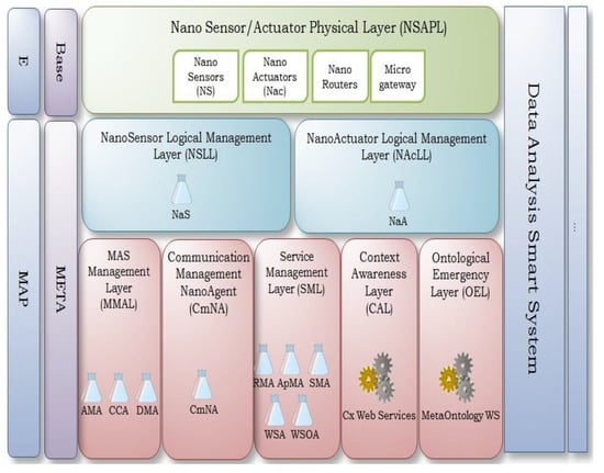
Figure 1.
ARMNANO middleware [2].
The base-level in ARMNANO is named NSAPL. It contains physical devices such as the NS, NA, Ro, and the microgateway. Then, the abstract views of the nanodevices in the NSAPL layer are deployed as logical agents, called NaS and NaA, in the metalevel. Elsewhere, at the meta-level, ARMNANO has five layers, which are MMAL, CmNA, SML, CAL, and OEL, that provide services with respect to context characterization and cloud connection, among other things.
3.1. Autonomic Cycles in ARMNANO
ARMNANO is composed of three ACs [5], which are deployed in the DASS. An AC has been defined in previous works as a group of data analysis tasks that work together to achieve an objective [28]. Each task has a different role, some to monitor, others to analyze, and others to make decisions about the process. This concept has been used in different fields [29,30,31]. In the context of ARMNANO, these ACs are the CTM that configures the nanodevices of the context in order to reach certain goals; the OTM that is executed to optimize the behavior of the nanodevices; and finally, the FTM that is invoked when there is a catastrophic change in the context in order to fix/determine the new environmental variables to reach in the nano-environment.
In the following, we detail the CTM AC. We consider this AC because it is the first input we obtained from the context under observation. In particular, this AC is responsible for determining the NS configuration to be used when deploying ARMNANO in a current application case. Thus, it is responsible for solving the combinatorial optimization problem that lies behind that objective.
3.2. Description of the CTM AC
This AC must determine the NSs to be deployed for the specific data analysis tasks that are carried out in the context (See Figure 2). It is composed of four tasks, as defined in [5]: Task 1 contemplates the most basic action in the AC, the measurement of the variables, Vi. Task 2 performs the authentication of this data, to send only truthful information to the DASS server, Tasks 3 and 4 involve more complex actions, which are outlined in detail later.
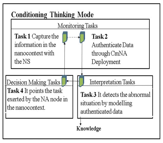
Figure 2.
Tasks for the CTM-AC.
3.3. Definition of the Tasks
ARMNANO has specific data analytic tasks in each AC. In Table 1, we describe the tasks of the CTM-AC.

Table 1.
Definition of the tasks for the CTM-AC.
Task 1, Capture the information in the nanocontext with the NS: this task is specific to the NSs deployed in the observed space. This task collects the data in the nanocomposed context. The architecture should discern the NS distribution. Additionally, it must assign a mode of communication for the NSs, which can be electromagnetic or molecular-based communication [2].
Task 2, Authenticate data through the CmNA deployment: the main aim of the authentication is to discard noise, false positives, and true negatives. If the data is already authenticated, then it passes to Task 3. This task applies the Authentication Data Protocol (ADP). Specifically, these tasks apply the ADP that consists of two levels. The 1st level analyzes the typical metrics of the data, such as the average, standard deviation, and variance. The 2nd level applies the Maximum Likelihood Estimation (MLE) model to determine the quality of the data source.
Task 3, Detect the abnormal situation by modelling authenticated data: this task uses the MLE model or other Machine Learning (ML) techniques, or a combination of them, to study the abnormal situations.
Task 4, Define the action exerted by the NA node in the nanocontext: a command defined by this AC is executed in the DASS, so that the NA node performs the actions. Some of these actions can be delivering medicament, destroying a fatty spot, localized organelle reparation, or cutting a specific internal spot. This node is devoted to only one function, such as cutting, moving, shifting, tapping, etc. The data source is the output of the models generated by the ML techniques in the previous task.
3.4. Genetic Algorithms (GA)
A GA is a metaheuristic based on the process of natural selection, which is commonly used to solve optimization problems. It uses biologically inspired operators, such as mutation and crossover, to generate high-quality solutions. A GA is composed of a population of individuals (candidate solutions to an optimization problem) [32]. Each individual has a set of properties (they define its chromosome), which determine its quality using a fitness function. The GA makes the evolution of the population in an iterative process (each iteration is called a generation). In each generation, the quality of each individual in the population is evaluated using the fitness function (normally, it is the objective function of the optimization problem to solve). The best individuals are selected, and each chromosome is modified using the genetic operators. In this way, a new generation is built to be used in the next iteration. Frequently, the algorithm ends according to a maximum number of generations, or when a good fitness value has been reached.
4. Results
Herein, we expose the instantiation of the CTM AC to study the NS deployment problem in the context of health solutions to an affected person or group of people.
4.1. Description of the Case Study
In the eHealth solutions field, there are plenty of specific sub-fields for applications; nonetheless, one of the most interesting is related to hepatic diseases, meaning those diseases connected to liver’s failure. Actual statistics demonstrate that individuals increased their alcohol consumption in the years 2020 and 2021, worldwide [33,34], which is generating several diseases linked to the liver [35,36].
We are going to test our approach on a dataset that defines people of different ages and genders to obtain a “big picture” and a “fine view” depending on the data used. Our data set includes 347 individuals with respect to five indicators of liver status. Four of them are enzymes and one is the Mean Corpuscular Volume (MCV). These variables are represented in Table 2 with their normal range.
Table 2.
Measured variables in the dataset to define the liver status.
SGOT enzyme: is an enzyme delivered when there is a tissue damage. Its concentration increases drastically in cases of wound or damage. A magnitude in 50 units/L for men or 45 for women indicates damage.
SGPT enzyme: is an enzyme that is produced in several organs, but its major concentration is found in the liver. The higher the concentration of this enzyme, the greater the tendency for liver damage.
ALKPHOS enzyme: its function is to catalyze the hydrolysis of the phosphate in the serum at alkaline pH. ALKPHOS is a specific variable for the liver.
Gammagt enzyme: measurements above 30 IU/L are directly connected to liver damage.
MCV: it is a measurement of the volume of the cell (measured in femtoliters, fL). Above the 90 fL level is considered macrocytic anemia.
To prove the capabilities of the 3rd task in the CTM AC, we consider only the ALKPHOS and MCV, for several reasons, including that the selection criteria to identify liver damage is when the enzyme concentration (any of them) is abnormally high, which can be determined using ALKPHOS (chemical compound) and MCV (geometric feature). They represent two different things measured in the same system, giving heterogeneity to our approach, as well as handling less information and discarding possible sources of errors.
Based on the design of the ARMNANO, a set of NSs is locally injected into the patient´s liver to perform the measurements. The NS nodes will track the two variables previously defined. The collected data concerning the context follow the characteristics required by the CTM AC regarding the format (units, etc.), etc.
4.2. Case Study 1: Liver Status in a Unisensor System
Herein, we consider that a regular alcohol drinker is consuming a certain number of glasses of alcohol, of any type, on a daily basis. He has gone to a Hepatologist to check his liver condition, although he has not had evidence of drastic liver failure, or any indication of pain. In this case, given that there is no previous register of this patient, there is a first analysis considering the MCV and ALKPHOS values.
The CTM AC will consider the deployment of one nanosensor that measures the two variables in the liver of the patient. Hence, we aim to determine the distance in the liver (DCH) where the damage is bigger to apply a localized treatment.
Figure 3 outlines the specific tasks of the AC for this problem. Each task requires ML techniques or data analysis.
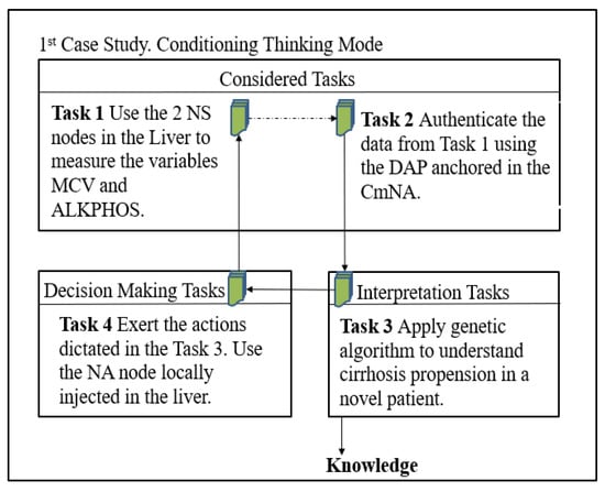
Figure 3.
Instantiation of the CTM AC to the 1st Case Study.
Task 1, Capture the information in the nanocontext with the NS: we deploy only one NS to measure the ALKPHOS and MCV.
Task 2, Authenticate data through the CmNA deployment: we apply the ADP of the ARMNANO to each measured variable.
Task 3, Apply the GA to understand the propensity for cirrhosis in a novel patient: we apply a GA to optimize the DCH variable due to the liver damage (see ranges in Table 2).
Task 4, Define the action exerted by the NA node in the nanocontext: it exerts the command determined in Task 3.
4.3. Case Study 2: Liver Status in Multisensor System
Herein, the same patient is treated as in case 1, but several NSs are deployed, thus conforming a multisensor (NS > 1) system, where each NS tracks the ALKPHOS and MCV simultaneously. It generates plenty of data, thus deploying a more aware view of the patient’ liver. A multisensor system requires specific optimum parameter settings depending on the number of NSs (see Figure 4).
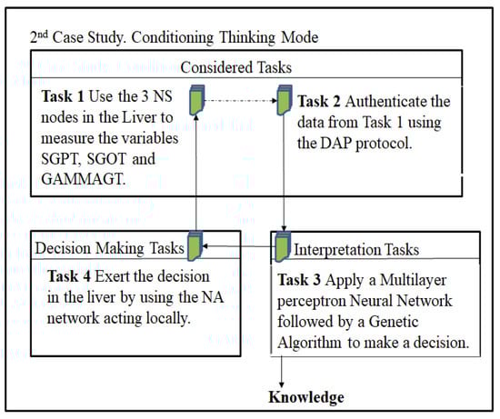
Figure 4.
Instantiation of the CTM AC for the 2nd Case Study.
Task 1, Use the NSs multisensor systems in the liver to measure the ALKPHOS and MCV: we measure the targeted variables using the NSs multisensor nodes.
Task 2, Authenticate the data from Task 1 using the ADP protocol: the ADP is executed to find out the appropriate data values in the measured variables.
Task 3, The CTM AC will consider the deployment of three NSs, five NSs, ten NSs, twenty NSs and thirty NSs in the liver of the patient. Hence, we aim to determine the distance in the liver (Distance from the end of the liver to the periphery, DCH) to apply a localized treatment.
Task 4, Exert the decision in the liver by using the NAs acting locally: it comprises the palliative action of the NAs to decrease the liver issue, for instance, to inject inhibitors of the enzyme ALKPHOS.
5. Numerical Results and Analysis
5.1. Specification of the Genetic Algorithm
A chromosome is defined as a vector of real numbers, with a size equal to 2, whose elements will be: ALKPHOS, MCV and DCH:
where the general clinical ranges for a healthy liver are between 44 ≤ ALKPHOS ≤ 200 and 80 ≤ MCV ≤ 140. On the other hand, the ideal values of DCH to accurately determine the status of the liver must be 0 ≤ DCH ≤ 160,000 (There is an equivalence between this extreme value of DCH with the maximum longitudinal value of the liver (14.5 cm)). We apply the evolving capabilities of the GA to determine whether, with these sensors, we can sense the ALKPHOS and MCV variables that define a good value of DCH to monitor possible damage in the liver. The objective function in our case determines the DCH based on the ALKPHOS and MCV variables. According to the literature, this function is [35,36,37]:
where the constant 0.05 is used to remove the units of the variables. The optimization occurs when the objective function is minimized (𝑚𝑖n(𝐹𝐹)), which means that we have values sensed of the ALKPHOS and MCV that allow for determining a good value for DCH.
On the other hand, for the evolution of the chromosome, we use a directed mutation to substitute the values of the elements of the chromosome randomly with those existing in the databases of the context (monitored patient).
For the hyperparameter optimization of the GA has been used the next set of values:
- Number of generations: [10, 50, 100, 150, 200]
- Population size: [10, 30, 50, 70, 100]
5.2. Case Studies
In the case studies, we are going to determine if it is possible, with the sensors, to capture the two variables of interest in a patient, to obtain a DCH that allows for monitoring the status of his/her liver. To do so, we conduct several simulations for different datasets with the information of the patients, in a case of a healthy patient taken from [15], and in others with diseased livers (cases of alcoholics (taken from [36])) and cases of other diseases (taken from [37])).
Case 1:
This is the first test case using a single sensor per variable (1 NS). We run the hyperparameter optimization every time we launch the GA. For example, the best values for each parameter for case 1 with the dataset [15] (it is the case of non-liver sick) are shown in Table 3.
Table 3.
Parameters of the GA for case 1.
The system with one NS was executed, and the best chromosome obtained is shown in Table 4, with the minimum best score (DCH).
Table 4.
The best individual found in case 1 for the dataset [15].
According to these results, the best distance from one end of the liver to the periphery, using the values of ALKPHOS and MCV for one of the patients in this dataset, is 24,225. This means that with one NS, the liver of that patient can be monitored without problem.
Now, we test our technique on the other two diseased liver datasets. Table 5 shows the results obtained with our GA for one NS.
Table 5.
The best individual found in case 1 for datasets [36,37].
Table 5 reveals two phenomena. For the first dataset, it is possible to obtain a very large DHC for the monitored patient; that is, it obtains values on the periphery of the liver to analyze its status. This indicates that a single sensor can be injected. However, the most relevant is that, in the second dataset, our GA cannot achieve a DCH, even in its periphery, to monitor this patient, which indicates that we must try with more sensors (objective of case study 2).
Case 2:
In this case study, the idea is to determine the appropriate number of sensors to be able to monitor a sick patient. In particular, we are going to use several patients from the dataset [37], which could not be monitored with one NS. On the other hand, in this case, the length of the chromosome is variable, so its length n depends on the number of NS used in that GA run. Thus, the chromosome t is represented as a vector of real numbers, with a size equal to n.
Chromosome = [ALKPHOS1, MCV1, DCH1, ALKPHOS2, MCV2, DCH2, …, ALKPHOSn, MCVn, DCHn]
The objective function, in this case, is given by:
The hyperparameter optimization of the GA is conducted for each GA run with a different n (multisensor system) for n equal to three NSs, five NSs, ten NSs, and twenty NSs. The best results (individual) for each run are shown in Table 6.
Table 6.
The best individual found in case 2 for the dataset [37].
Table 6 indicates that at least four sensors are required to correctly monitor the liver. In addition, it indicates that having more than five sensors does not improve the accuracy of the liver monitoring results.
Something interesting to determine is how to implement the NS. For example, in the case of four NSs, considering the best individual, the liver can be divided into four zones (see Figure 5): A, from 0 to 40,000; B, from 40,000 to 80,000 au; C, from 80,000 to 120,000 au; and D, from 120,000 to 156,500. Therefore, each sensor must be injected into these areas to obtain the data from the damaged area.
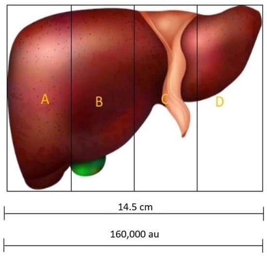
Figure 5.
Liver bisected in 4 regions to inject the NSs in each one.
The behavior of a multisensor system depends on the amount of NSs that are tracking the liver. In addition, it determines the zones where the NSs will be deployed (see Figure 5). On the other hand, a small o big number of NSs is not indicative of an optimal DCH, it is a number that must be determined (in our case, four NSs or five NSs). In our example of Figure 5, scaling to the size of the liver in a man of 14.5 cm, the GA determines the zones in which to inject the sensors in a specific sick patient. A bigger data volume would reveal a more precise zone, but a greater amount of NSs is required.
As shown in Table 7, we conducted a test for a group of patients from the dataset [37] with liver diseases. We see that the minimum number of NSs required by a patient is three, but for the vast majority, five NS is enough to follow the state of their diseased livers.
Table 7.
The best individual found in case 2 for the dataset [37] and different patients.
In general, for a patient with more complex liver disease, a more accurate view of the liver is required (involves more NSs). With more NSs, a more precise view of the liver can be obtained (more areas can be monitored) to follow all the damaged parts of the liver.
Consequently, task 4 of the CTM AC determines the NSs to be injected and in which areas of the liver. Task 4 continues to observe the liver, and if it determines that it must recalculate the NSs, then it does so in the next iteration.
6. Conclusions
Through the DASS, it has been possible to deploy ARMNANO in a medical context, which is often complicated. In particular, this work implemented the CTM AC to determine the number of NSs to be deployed to supervise the liver in patients.
The problem of the determination of the optimal number of NSs to monitor the liver in a patient was analyzed as an optimization problem. The first case study is for one NS, and as a multisensor system in case study 2. In this second case study, the capability of the GA to estimate the number of NSs is evaluated: three, four, five, etc. With one NS, only very simple cases of patients (not liver-sick, etc.) can be monitored. On the contrary, the multisensor system can evolve with the GAs to determine the correct number of NSs to be used and, additionally, the zones where the NSs must be deployed in the liver.
Future works will analyze the application of this methodology in other case studies, application domains, etc. In addition, it must be integrated with the rest of the DASS components and the ARMNANO middleware. Finally, returning to the comment from the previous section on how to deploy/implement the NSs, future work should specify the procedure to determine where to place the NSs following, for example, the medical bases of the problem under study (in our case, to monitor the state of the liver).
Author Contributions
Conceptualization, A.L. and J.A.; methodology, J.A.; software, A.L.; validation, A.L. and J.A.; formal analysis, A.L. and J.A.; writing, A.L. and J.A. All authors have read and agreed to the published version of the manuscript.
Funding
This research received no external funding.
Data Availability Statement
No new data were created, Datasets used are from [15,36,37].
Conflicts of Interest
The authors declare no conflict of interest.
References
- García-Haro, J.; García-Sanchez, S.; Canovas-Carrasco, S. The IEEE 1906.1 Standard: Nanocommunications as a New Source of Data. In Proceedings of the ITU Kaleidoscope: Challenges for a Data-Driven Society, Nanjing, China, 27–29 November 2017. [Google Scholar]
- Lopez-Pacheco, A.; Aguilar, J. NANO-Communication Management System for Smart Environments. Rev. Venez. Comput. 2018, 5, 12–22. [Google Scholar]
- García-Haro, J.; García-Sanchez, S.; Canovas-Carrasco, S. The IEEE 1906.1 Standard: Some Guidelines for Strengthening Future Normalization in Electromagnetic Nanocommunications. IEEE Commun. Stand. Mag. 2018, 2, 26–32. [Google Scholar]
- Lopez-Pacheco AAguilar, J.; Puerto, E.; Garcia, R. An ontological model based on the ontology driven architecture paradigm for a middleware in the management of nano-devices in a smart environment. J. Phys. Conf. Ser. 2019, 1386, 012138. [Google Scholar] [CrossRef]
- Lopez-Pacheco, A.; Aguilar, J. Data Analysis Smart Systems in a Nanodevices Based Middleware. Contemp. Eng. Sci. 2018, 11, 4665–4679. [Google Scholar] [CrossRef]
- Lopez-Pacheco, A.; Aguilar, J. Autonomic Reflective Middleware for the Management of NANOdevices in a Smart Environment (ARMNANO). Curr. Anal. Commun. Eng. 2019, 2, 56–63. [Google Scholar]
- Millery, M.; Ramos, W.; Lien, C.; Aguirre AKukafka, R. Design of a Community-Engaged Health Informatics Platform with an Architecture of Participation. AMIA Annu. Symp. Proc. 2015, 2015, 905–914. [Google Scholar]
- Divya, V.; Kumar, S. A Comprehensive Review on Various Signal Conditioning Methods in Nano-Sensor Based Applications. J. Comput. Theor. Nanosci. 2020, 17, 2043–2050. [Google Scholar] [CrossRef]
- Zamuda, A.; Zarges, C.; Stiglic, G.; Hrovat, G. Stability selection using a genetic algorithm and logistic linear regression on healthcare records. In Proceedings of the Genetic and Evolutionary Computation Conference Companion, Berlin Germany, 15–19 July 2017. [Google Scholar]
- Wilmer, C. Genetic Algorithm Design of MOF-based Gas Sensor Arrays for CO2-in-Air Sensing. Sensors 2020, 20, 924–936. [Google Scholar]
- Ghaheri, A.; Shoar, S.; Naderan, M.; Shahabuddin, S. The Applications of Genetic Algorithms in Medicine. Oman Med. J. 2015, 30, 406–416. [Google Scholar] [CrossRef]
- Kumar, A.; Tyagi, P.; Bhatnagar, A. Genetic Algorithm and their applicability in Medical Diagnostic: A Survey. Int. J. Sci. Eng. Res. 2016, 7, 1143–1145. [Google Scholar]
- Alpers, S.; Skogen, J.; Maeland, S.; Pallesen, S.; Rabben, A.; Lunde, L.; Fadnes, L. Alcohol Consumption during a Pandemic Lockdown Period and Change in Alcohol Consumption Related to Worries and Pandemic Measures. Int. J. Environ. Res. Public Health 2021, 18, 1220. [Google Scholar] [CrossRef] [PubMed]
- Jongwook, J.; Byung-Gook, P.; Hyungcheol, S. Investigation of Thermal Noise Factor in Nanoscale MOSFETs. J. Semicond. Technol. Sci. 2010, 10, 225–231. [Google Scholar]
- Asrani, S.; Devarbhavi, H.; Eaton, J.; Kamath, P. Burden of liver diseases in the world. J. Hepatol. 2019, 70, 151–171. [Google Scholar] [CrossRef]
- Leong, Y.; Tan, E.; Leong, S.; Koh, C.; Nguyen, L.; Chen, J.; Xia, K.; Ling, X. Where nanosensors meet machine learning: Prospects and challenges in detecting Disease X. ACS Nano 2022, 16, 13279–13293. [Google Scholar] [CrossRef]
- Akyol, D.; Orgulu, B. Towards a Different Architecture in Cooperation with Nanotechnology and Genetic Science: New Approaches for the Present and the Future. Archit. Res. 2014, 4, 1–12. [Google Scholar]
- Dorj, U.; Lee, M.; Choi, J.; Lee, Y.; Jeong, G. The Intelligent Healthcare Data Management System Using Nanosensors. J. Sens. 2017, 2017, 7483075. [Google Scholar] [CrossRef]
- Bushko, R. Future of eHealth: Can Consumers Cure Themselves? Stud. Health Technol. Inform. 2009, 149, 178–184. [Google Scholar]
- Mehr, H.; Craven, M.; Leono, A.; Keenan, G.; Cronin, A. A universal system for digitization and automatic execution of the chemical synthesis literature. Science 2020, 370, 101–108. [Google Scholar] [CrossRef]
- Niroumand, H.; Zain, M.; Jamil, M. Statistical Methods for Comparison of Data Sets of Construction Methods and Building Evaluation. Procedia-Soc. Behav. Sci. 2013, 89, 218–221. [Google Scholar]
- Severson, T.; Besur, S.; Bonkovsky, H. Genetic factors that affect nonalcoholic fatty liver disease: A systematic clinical review. World J. Gastroenterol. 2016, 29, 6742–6756. [Google Scholar] [CrossRef]
- Mejía-Salazar, J.; Rodrigues Cruz, K.; Materón Vásques, E.; Novais de Oliveira, O., Jr. Microfluidic Point-of-Care Devices: New Trends and Future Prospects for eHealth Diagnostics. Sensors 2020, 20, 1951. [Google Scholar] [CrossRef]
- Chakravarthy, V.; Hakkim Devan Mydeen, P.; Seenivasan, M. Study on Internet of Nanotechnology (IoNT) in a Healthcare Monitoring System, In Handbook of Research on Nano-Drug Delivery and Tissue Engineering: Guide to Strengthening Healthcare Systems; Rajakumari, R., Hanna, J., Sabu, T., Nandakumar, K., Eds.; Apple Academic Press: New York, NY, USA, 2022. [Google Scholar]
- Mujawar, M.; Gohel, H.; Bhardwaj, S.; Srinivasan, S.; Hickman, N.; Kaushik, A. Nano-enabled biosensing systems for intelligent healthcare: Towards COVID-19 management. Mater. Today Chem. 2020, 17, 100306. [Google Scholar] [CrossRef] [PubMed]
- Kedar, N.; Ravindharan, E.; Paramananda, J. Applications of IoT in Health Care: Challenges and Benefits. In IoT Applications, Security Threats, and Countermeasures; Padmalaya, N., Niranjan, R., Ravichandran, P., Eds.; CRC Press: Boca Raton, FL, USA, 2021. [Google Scholar]
- Singh, K.; Nayak, V.; Singh, J.; Singh, R. Nano-enabled wearable sensors for the Internet of Things (IoT). Mater. Lett. 2021, 304, 130614. [Google Scholar] [CrossRef]
- Vizcarrondo, J.; Aguilar, J.; Exposito, E.; Subias, A. MAPE-K as a service-oriented architecture. IEEE Lat. Am. Trans. 2017, 15, 1163–1175. [Google Scholar]
- Sánchez, M.; Aguilar, J.; Cordero, J.; Valdiviezo-Díaz, P.; Barba-Guamán, L.; Chamba-Eras, L. Cloud Computing in Smart Educational Environments: Application in Learning Analytics as Service. In New Advances in Information Systems and Technologies; Rocha, Á., Correia, A., Adeli, H., Reis, L., Mendonça Teixeira, M., Eds.; Advances in Intelligent Systems and Computing; Springer: Berlin/Heidelberg, Germany, 2016; Volume 444, pp. 993–1002. [Google Scholar]
- Aguilar, J.; Garcès-Jimènez, A.; Gallego-Salvador, N.; Gutierrez De Mesa, J.; Gomez-Pulido, J.; Garcìa-Tejedor, A. Autonomic Management Architecture for Multi-HVAC Systems in Smart Buildings. IEEE Access 2019, 7, 123402–123415. [Google Scholar] [CrossRef]
- Morales, L.; Ouedraogo, C.; Aguilar, J. Experimental comparison of the diagnostic capabilities of classification and clustering algorithms for the QoS management in an autonomic IoT platform. Serv. Oriented Comput. Appl. 2019, 13, 199–219. [Google Scholar] [CrossRef]
- Aguilar, J. Definition of an energy function for the random neural to solve optimization problems. Neural Netw. 1998, 11, 731–737. [Google Scholar]
- I. S. 1906.1; IEEE Recommended Practice for Nanoscale and Molecular Communication Framework. IEEE Communications Society: New York, NY, USA, 2015.
- Russell, A. Rough Consensus and Running Code’ and the Internet-OSI Standards War. IEEE Ann. Hist. Comput. 2006, 28, 48–61. [Google Scholar] [CrossRef]
- Scorza, M.; Elce, A.; Zarrilli, F.; Liguori, R.; Amato, F.; Castaldo, G. Genetic Diseases That Predispose to Early Liver Cirrhosis. Int. J. Hepathol. 2014, 2014, 713754. [Google Scholar] [CrossRef]
- Moon, A.; Singal, A.; Tapper, E. Contemporary Epidemiology of Chronic Liver Disease and Cirrhosis. Clin. Gastroenterol. Hepatol. 2020, 18, 2650–2666. [Google Scholar] [CrossRef]
- Bellentani, S.; Tiribelli, C.; Saccoccio, G.; Sodde, M.; Fratti, N.; De Martin, C.; Cristianini, G. Prevalence of Chronic Liver Disease in the General Population of Northern Italy. The Dionysos Study. Hepatology 1994, 20, 1442–1450. [Google Scholar] [CrossRef] [PubMed]
Disclaimer/Publisher’s Note: The statements, opinions and data contained in all publications are solely those of the individual author(s) and contributor(s) and not of MDPI and/or the editor(s). MDPI and/or the editor(s) disclaim responsibility for any injury to people or property resulting from any ideas, methods, instructions or products referred to in the content. |
© 2023 by the authors. Licensee MDPI, Basel, Switzerland. This article is an open access article distributed under the terms and conditions of the Creative Commons Attribution (CC BY) license (https://creativecommons.org/licenses/by/4.0/).