Article

Iterative Image Reconstruction Algorithm with Parameter Estimation by Neural Network for Computed Tomography

Institute of Biomedical Sciences, Tokushima University, 3-18-15 Kuramoto, Tokushima 770-8509, Japan
*
Author to whom correspondence should be addressed.
Algorithms 2023, 16(1), 60; https://doi.org/10.3390/a16010060
Submission received: 13 December 2022 / Revised: 3 January 2023 / Accepted: 13 January 2023 / Published: 16 January 2023

Abstract

:
Recently, an extended family of power-divergence measures with two parameters was proposed together with an iterative reconstruction algorithm based on minimization of the divergence measure as an objective function of the reconstructed images for computed tomography. Numerical experiments on the reconstruction algorithm illustrated that it has advantages over conventional iterative methods from noisy measured projections by setting appropriate values of the parameters. In this paper, we present a novel neural network architecture for determining the most appropriate parameters depending on the noise level of the projections and the shape of the target image. Through experiments, we show that the algorithm of the architecture, which has an optimization sub-network with multiplicative connections rather than additive ones, works well.

1. Introduction

Computed tomography (CT) can be thought of in terms of a linear inverse problem wherein one estimates tomographic images from a measured projection and a known projection operator [1,2,3,4,5,6]. Although filtered back-projection, which is an analytical method, is widely used for image reconstruction in medical CT scanners, iterative image reconstruction [2,5,7,8,9] better meets modern requirements for practical use. The iterative image reconstruction method is based on an optimization algorithm and can obtain an image with relatively few artifacts from noisy projection data. The maximum-likelihood expectation-maximization (MLEM) algorithm [2], a typical iterative image reconstruction algorithm, is known to minimize the Kullback–Leibler (KL) divergence [10] of the measured and forward projections.
Since the objective function of a minimization problem for CT affects the quality of the reconstructed images, a rational design of the function is essential. Our research group previously presented a two-parameter extension of the power-divergence measure (PDM) [11,12,13,14], called EPDM, and proposed an iterative image reconstruction method [15] based on minimization of EPDM as an objective function, i.e., the PDEM algorithm. Note that, because the KL-divergence is a special case of the EPDM family, PDEM is a natural extension of MLEM. The PDEM algorithm can produce a high-quality reconstructed image by adjusting the values of the parameters depending on the degree of noise in the measured projection.
PDEM is derived from a nonlinear differential equation using the dynamical method [16,17,18,19,20,21] applied to tomographic inverse problems [22,23,24,25,26,27], which means that a discretization of the differential equation by using a first-order expansion of the vector field leads to an equivalent iterative formula. A theoretical result from the previous study [15] is that the global stability of an equilibrium corresponding to the desired solution observed in the continuous-time system is guaranteed by the Lyapunov theorem [28]. Furthermore, numerical experiments have shown that the appropriate parameters depend on the level of projection noise. As a natural conjecture, the appropriate parameters also depend on the shape of the image to be reconstructed, so one may consider whether it is possible to develop a method for estimating the parameters from the measured projection.
In recent years, many studies have incorporated deep-learning approaches for parameter estimation in iterative algorithms [29,30,31,32,33,34,35]. The well-known methods of ADMM-Net [32] and ISTA-Net [34] embed an iterative algorithm into a deep neural network by using the alternating direction method of multipliers [36] and the iterative shrinkage thresholding algorithm [37], respectively. Some of these studies have used recurrent neural networks (RNNs) in which convolutional sub-networks for estimating parameters are used in each iterative calculation and the iterative calculations are intertwined [29,33]. The complexity of the networks increases in proportion to the number of iterative calculations, but the risk of the vanishing gradient problem [38] occurring is low because the calculations are implemented as residual blocks [39]. The ideas behind this neural network architecture (referred to below as learned optimization; LO) have been organized by Andrychowicz et al. [40], and LO has been actively improved in terms of its design, training method, performance, and operation [41,42,43,44,45,46,47]. In particular, this technique has been applied to the field of medical imaging, especially the problem of compressed sensing in magnetic resonance imaging [48,49,50]. Zhang et al. [51] used it together with Nesterov’s acceleration [52] to estimate parameters associated with the regularization term for compensating for a lack of signals.
In this paper, we propose a novel neural-network architecture that estimates the values of parameters in the PDEM algorithm by using projection data. The proposed architecture is similar to LO because it has two subsystems for estimating parameters and iterative operations. Following the naming convention of Andrychowicz et al., we call these subsystems the optimizer and optimizee, respectively. Unlike conventional LO, the subsystems are completely separated in our system, and the network architecture is more straightforward than that of RNNs. The traditional LO estimates parameters by using the results of each iterative calculation, whereas our architecture uses only projection data. Nevertheless, the experimental results illustrate that our method works well. Moreover, the optimizee has a different structure than the traditional optimizee, with multiplicative rather than additive connections.

2. Problem Description

We assume that the measured projection y R + I in computed tomography is acquired according to the linear model
y = A x + δ
where A R + I × J , x R + J , and δ R I are a projection operator, target image, and noise, respectively, with R + denoting the set of nonnegative real numbers. The purpose of iterative reconstruction is to obtain a high-quality image similar to the target image by solving an initial value problem consisting of a difference equation or an equivalent iterative algorithm. Recently, a novel iterative image reconstruction algorithm [15], which is based on minimization of the EPDM as an objective function of the measured and forward projections, has been developed:
z j ( k + 1 ) = z j ( k ) f j ( z ( k ) ; y , λ )
with
f j ( z ; y , λ ) : = i = 1 I A i j y i A i z α γ i = 1 I A i j A i z A i z α γ
for j = 1 , 2 , , J and k = 0 , 1 , 2 , , K 1 with z ( 0 ) = x 0 R + J , where A i and A i j indicate the ith row vector and the element in the ith row and jth column of the matrix A, respectively, and γ > 0 and α 0 are parameters that are collectively referred to as λ : = γ , α . The PDEM algorithm described in Equation (2) can be rewritten as
z ( k + 1 ) = z ( k ) f ( z ( k ) ; y , λ ) ,
with f : = ( f 1 , f 2 , , f J ) , where the symbol ⊙ denotes the Hadamard product and the superscript ⊤ stands for the transpose.
The purpose of this paper is to construct a system that estimates the most appropriate values of λ in the PDEM algorithm from the projection y by using a deep-learning approach.

3. Proposed Method

Our goal is to design a system for estimating an appropriate set of parameters λ from the projection y by using supervised learning on a deep neural network, described by
Λ : R + I R 2 ; y λ .
Since it is complicated to prepare a large set of appropriate parameters as a teaching dataset, we chose to use the following network architecture,
Θ ( y ) : = Ω ( y , Λ ( y ) )
where
Ω ( y , λ ) : = p p p K ( x 0 )
with
p ( z ) : = z f ( z ; y , λ )
as illustrated in Figure 1, and convert the neural network’s output into a reconstructed image. This architecture allows us to use true images or high-quality reconstructed images as teaching data. The subsystem Ω as an optimizee produces a reconstructed image z ( K ) by iterating the formula in Equation (2) K times, as shown in Figure 2. Note that it does not include any training parameters. The whole system Θ is implemented as a deep neural network and the training parameters of the subsystem Λ are automatically adjusted through the backpropagation procedure.
Although the depth of the computational graph of Θ increases in proportion to the number of iterations K, the optimizee Ω can be considered to be the residual blocks that can then be configured with multiplicative connections, as shown in Figure 2 and Figure 3, which is expected to reduce the risk of the vanishing gradient problem occurring. The well-known residual blocks can be described in terms of a difference equation
w j ( k + 1 ) = w j ( k ) + g j ( k , w ( k ) ) ,
for j = 1 , 2 , , J and k = 0 , 1 , , which is obtained by applying the (additive) Euler method with a step size of 1 to the differential equation
d v j ( t ) d t = g j ( t , v ( t ) )
with w j ( 0 ) = v j ( 0 ) . On the other hand, applying the multiplicative Euler method [53] to Equation (8) yields the difference equation
u j ( k + 1 ) = u j ( k ) exp g j ( k , u ( k ) ) u j ( k )
for j = 1 , 2 , , J and k = 0 , 1 , with u j ( 0 ) = v j ( 0 ) . Both residual blocks have shortcut edges that may help reduce the risk of the vanishing gradient problem. Indeed, the system in Equation (2) can be derived by discretizing the differential equation
d x j ( t ) d t = x j ( t ) log f j ( x ( t ) ; y , λ ) ,
for j = 1 , 2 , , J and t 0 with x ( 0 ) = x 0 by using the multiplicative Euler method. The differential equation in Equation (10) is guaranteed by the Lyapunov theorem to converge globally to the desired solution when the algebraic equation in Equation (1) with δ = 0 has a solution.

4. Results and Discussion

In this section, we present the results of an experiment on the proposed system using 5000 pairs of input and teaching data generated by numerical simulations. We generated teaching data in the form of 64 × 64 -pixel images deformed by changing the attributes of each oval, i.e., its intensity, size, position, and rotation angle, from the Shepp–Logan phantom [54] shown in Figure 4a. The attributes were varied in the ratio ranges shown in Table 1 from that of the base phantom by using uniform random numbers. The MATLAB (MathWorks, Natick, MA, USA) function phantom [55] generated the images. To avoid generating extremely large or small ovals that should not be considered, some common deformation rates were chosen for one attribute in some of the sets of ovals in one phantom. The input data were projections calculated by Equation (1) by using a common projection operator A, projection noise δ , and the target image x as the corresponding teaching data. The projection operator A, represented as a matrix, was simulated on the basis of the Radon transform assuming parallel projections from 90 directions with 95 detectors, so I = 90 × 95 and J = 64 × 64 . The signal-to-noise ratio (SNR) for each projection was selected so as to be uniformly distributed in the range of 20 dB to 50 dB. Figure 5 shows the resulting experimental histogram of SNRs, while Figure 6 shows samples of learning data generated by the above procedure.
In the experiment, we designed the optimizer Λ to be a simple and typical network (Figure 7). The batch normalization layer [56] is supposed to stabilize learning, reduce the initial value dependence of the learning parameters, and speed up learning. The dropout layer [57] is used to suppress overfitting.
Since the first hidden layer is dense, it requires a massive number of training parameters, resulting in a vast computational cost for training. Therefore, designing a more efficient optimizer Λ is a future challenge.
The parameters γ and α are power exponents, and giving them excessive values makes the numerical operations unstable. However, in the process of automatically updating the learning parameters by using the backpropagation procedure, γ and α are given large values that temporarily exceed the tolerance of a stable calculation . We avoided this problem by setting an upper limit on the output values of the optimizer Λ .
We define the activation function of the output layer of Λ to be
h ( x 1 , x 2 ) : = 1.8 × ( sgm ( x 1 ) , sgm ( x 2 ) ) ,
where the function sgm is the standard sigmoid function. The coefficient of 1.8 for the sigmoid function, given as an upper bound for both parameters, is small enough not to cause numerical instability or affect the parameter estimation.
The learning conditions and hyperparameters were as follows. We used 4000 pairs of data for training and 1000 pairs different from them for validation. For the optimizee Ω responsible for image reconstruction, the number of iterations was K = 200 and an initial value was x 0 = ( 0.5 , 0.5 , , 0.5 ) . Note that the value of the maximum iteration number K was chosen to ensure a sufficient reconstruction quality and to properly observe the difference in the convergence characteristics between the PDEM and MLEM algorithms, as shown in the previous study [15]. The number of epochs and the batch size were 5000 and 64, respectively. We used the squared L2 norm as the loss function. The Adam algorithm [58] was used to minimize the loss function; its learning rate was set to 10 6 . The learning network was implemented using Python 3.9.7 and TensorFlow 2.8.0.

4.1. Results of Learning

Here, we present the experimental results of learning and show that the proposed network successfully learned the optimizer Λ .
Figure 8 shows the values of the loss function at each epoch. At the final epoch (the 6000th), the loss function for the training data shows a decreasing trend, while the one for the validation data converged, indicating that the learning was sufficient.
To evaluate the performance of the learned optimizer Λ , we validated it on a test dataset consisting of data not included in the training and validation datasets. The properties described below are common to all of the test datasets. We will discuss the results for five of the test data pairs shown in Figure 9. The first test data item ( = 1 ) was a pair of a projection y 1 with an SNR of 20 dB and the expected reconstructed image e 1 . In the second and third test data pairs ( = 2 and 3), the expected reconstructed images e 2 and e 3 equaled e 1 but with different Sn Rs of the projection. On the other hand, in the fourth and fifth test data pairs ( = 4 and 5), the expected reconstructed images e 4 and e 5 were different from e 1 and from each other, but the noise levels of the projections were 20 dB.
Figure 10 plots the evaluation function values
D ( , z ) : = e z 2
defined by the L2 norm of the difference between the th true image e and reconstructed image z when using the parameter λ ^ = ( γ ^ , α ^ ) estimated by the learned model Λ from the projection y with = 1 , 2 , , 5 . The results for the MLEM algorithm, i.e., the PDEM algorithm with λ = ( 1 , 1 ) , are displayed for comparison.
For the first test data pair ( = 1 ), due to the high noise level, the evaluation functions for both the MLEM and the proposed algorithm, which is the PDEM using the parameter values λ ^ 1 = ( 0.40 , 1.05 ) estimated by the optimizer Λ , do not decrease monotonically but rather start to increase at different iteration numbers, around k = 50 and 140, respectively. The proposed method decreases the evaluation function significantly in the last iteration compared with that of the MLEM algorithm. This result indicates that the optimizer Λ can estimate parameter values that, while not optimal, significantly improve image quality. The results for the second test data pair ( = 2 ), which has a different noise level than the first test data pair ( = 1 ), shows that the proposed method also reduces the evaluation function compared with the MLEM algorithm, but the difference is slight. We discuss the reason in the following subsection. The proposed method can significantly reduce the evaluation function when using the third test data pair ( = 3 ), which has weak noise. The reason for this is presumably that the power exponent parameter γ is a value that affects the step size in the discretization of the continuous dynamical system and that, when the noise is weak, a relatively large parameter is chosen for fast convergence to a value close to the true one. In fact, the estimated parameter γ ^ 3 is 1.64, which is larger than the others. The results for the fourth and fifth test data pairs ( = 4 and 5), where the projection contains a lot of noise, show a slight decrease in the value of the evaluation function, contrary to the results for the first test data pair ( = 1 ), where the SNRs of the projections are comparable. This result suggests that the optimal parameters also depend on the shape of the reconstruction target.
Figure 11 shows the contour maps of the evaluation function values of the reconstructed image z ( K ) for changes in the parameters γ and α according to the projection y . On all the test data, the optimizer Λ could estimate parameters that reduce the evaluation function value more than the MLEM algorithm. In the case of = 1 and = 3 , where significant improvements were observed, the region of suitable parameters is located far from ( γ , α ) = ( 1 , 1 ) corresponding to the parameter for MLEM, and the optimizer Λ succeeds in estimating the values around it. On the other hand, for = 2 , 4 , and 5, where the differences in the evaluation functions are slight, the optimal parameters are relatively close to ( 1 , 1 ) . In other words, these cases are problem settings in which the MLEM algorithm can achieve high performance. Even in such cases, our optimizer can estimate the parameters better than it can. The previous study suggested the possibility of a rough parameter estimation by using the noise level. Indeed, the results for = 1 , 4 , and 5 show similar trends in the contour plots for the same noise level, and the results for = 1 , 2 and 3 show a significant change in trend with the noise level. However, the optimal parameter values and contour maps depend not only on the noise level but also on the shape of the reconstruction target.

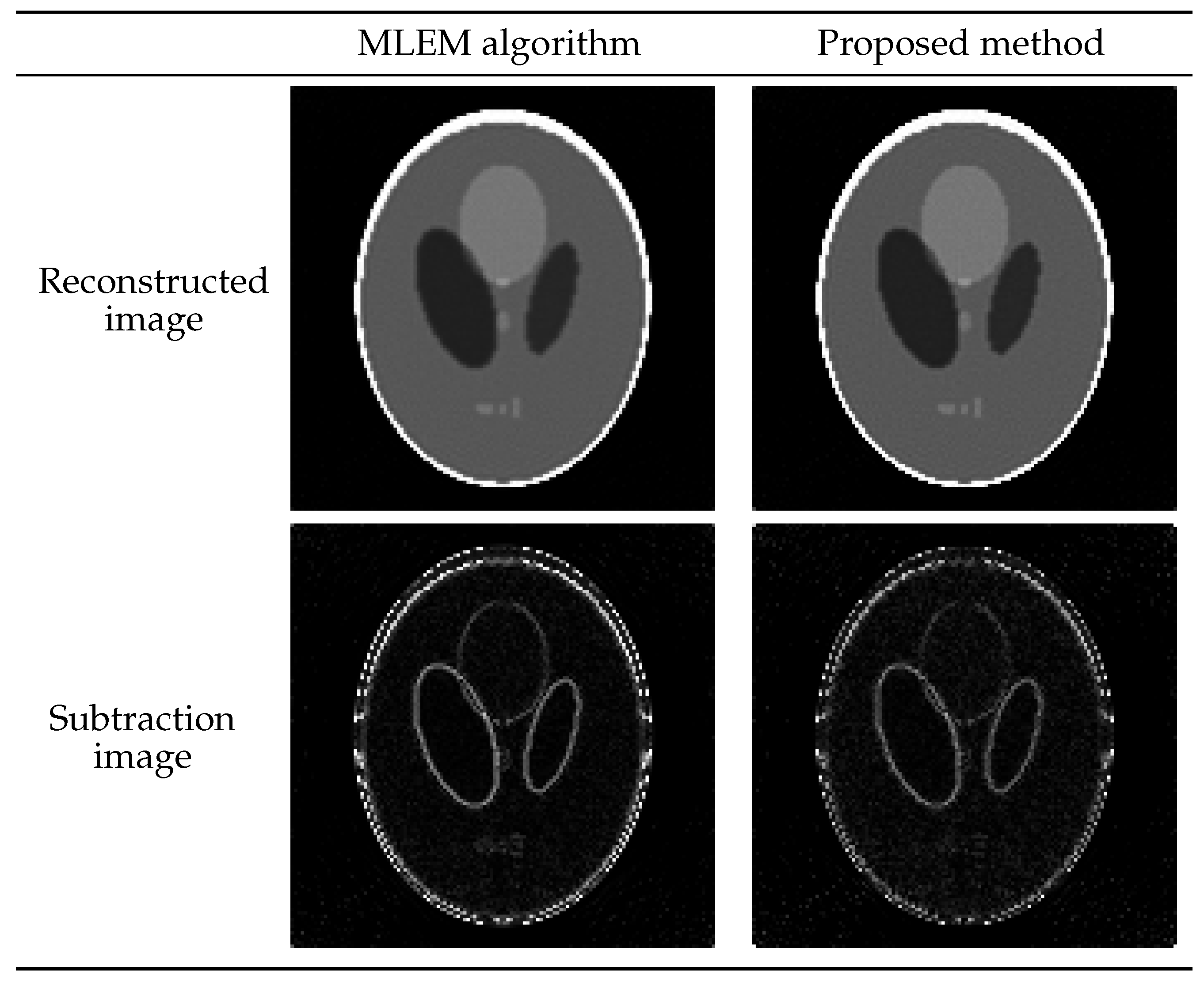
4.2. Application of Estimated Parameters to Reconstruction of Larger Images

Considering larger images and sinograms in practical CT applications, the significant increase in network size and training cost leads to problems of increased computer memory and computation time. To avoid these problems, we propose the following solution. First, a small reconstructed image and the corresponding projection are prepared as training data. These small-sized data are used to construct the optimizer Λ in a training manner. When estimating parameters from the original projection numbers, the projection is reduced to the same size as the training data and input to the optimizer. Then, the estimated parameters are used to reconstruct the image from the original projection. In this subsection, we verify the feasibility of this procedure by showing that the estimated parameters can be used to reconstruct a larger projection than that used for training.
We generated projections y 6 , y 7 , , y 10 , which were magnified versions of projections y 1 , y 2 , , y 5 . These projections were generated from phantoms e 6 , e 7 , , e 10 shown in Figure 12, which were enlargements of e 1 , e 2 , , e 5 . The projection noise level to be applied was the same as in the previous subsection. The number of projection directions was increased to 180 so that the inverse problem would not be unduly difficult due to the large image size 128 × 128 . In the proposed use case, the parameters are estimated on the basis of a smaller projection reduced from the larger projection, but here the procedure is inverted. That is, the image reconstruction of projection y for any = 6 , 7 , , 10 uses the parameter λ 5 estimated from its smaller version, projection y 5 .
Figure 13 plots the values of the evaluation function during reconstruction. The same trend as in Figure 10 is obtained when the parameters estimated from the reduced projection are diverted. The contour maps of the parameters shown in Figure 14 are also consistent with the trend in Figure 11, suggesting that it is possible to use the parameters estimated from the miniaturized projection. Although developing a method to reduce the size of the large original projection appropriately is required for actual use, the results show the possibility of a practical application.
The reconstructed and subtraction images from the true value on the test data = 6 and = 8 are shown in Figure 15 and Figure 16. The images reconstructed by the MLEM algorithm and their subtraction images are also shown for comparison. Comparing the reconstructed images for = 6 , it can be seen that the images of the proposed method significantly reduce the overall presence of granular artifacts. In the case of = 8 , the reproducibility of the contour area is high, which is why the evaluation function value is smaller than that of the MLEM algorithm. Thus, the proposed method worked exceptionally well.

5. Conclusions

We developed a system for estimating appropriate parameters for the projection to be reconstructed by employing deep learning on the PDEM algorithm, which has two parameters and is a generalization of various iterative image reconstruction methods. As a learning network, we proposed a structure that connects the optimizer, i.e., the estimation model, and the PDEM algorithm. This architecture is less complex than traditional learned optimization architectures employing RNNs and achieves satisfactory estimations of the parameters of the PDEM algorithm. Although, the appropriate parameters depend on the noise level of the projection and the shape of the phantom, the learned estimation system can estimate them for any projection.
Furthermore, we showed that an optimizer trained on small projections can estimate appropriate parameters for image reconstruction of a projection of a practical size, indicating that the proposed algorithm can be applied to practical problems with larger images and sinograms. This fact enables us to avoid a considerable increase in training costs when reconstructing a clinical CT image.

Author Contributions

Conceptualization, T.K. and T.Y.; Data curation, T.K. and T.Y.; Formal analysis, T.K.; Methodology, T.K. and T.Y.; Software, T.K.; Supervision, T.Y.; Validation, T.K. and T.Y.; Writing—original draft, T.K. and T.Y.; Writing—review and editing, T.K. and T.Y.; All authors have read and agreed to the published version of the manuscript.

Funding

This research was partially supported by JSPS KAKENHI, Grant Number 21K04080.

Data Availability Statement

All data used to support the findings of this study are included within the article.

Conflicts of Interest

The authors declare no conflict of interest regarding the publication of this paper.

References

  1. Ramachandran, G.N.; Lakshminarayanan, A.V. Three-dimensional reconstruction from radiographs and electron micrographs: Application of convolutions instead of Fourier transforms. Proc. Natl. Acad. Sci. USA 1971, 68, 2236–2240. [Google Scholar] [CrossRef] [PubMed] [Green Version]
  2. Shepp, L.A.; Vardi, Y. Maximum Likelihood Reconstruction for Emission Tomography. IEEE Trans. Med. Imaging 1982, 1, 113–122. [Google Scholar] [CrossRef] [PubMed]
  3. Lewitt, R.M. Reconstruction algorithms: Transform methods. Proc. IEEE 1983, 71, 390–408. [Google Scholar] [CrossRef]
  4. Natterer, F. Computerized tomography. In The Mathematics of Computerized Tomography; Springer: Berlin/Heidelberg, Germany, 1986; pp. 1–8. [Google Scholar]
  5. Stark, H. Image Recovery: Theory and Application; Academic Press: Washington, DC, USA, 1987. [Google Scholar]
  6. Hudson, H.M.; Larkin, R.S. Accelerated image reconstruction using ordered subsets of projection data. IEEE Trans. Med. Imaging 1994, 13, 601–609. [Google Scholar] [CrossRef] [Green Version]
  7. Kak, A.C.; Slaney, M. Principles of Computerized Tomographic Imaging; Society for Industrial and Applied Mathematics: Philadelphia, PA, USA, 2001. [Google Scholar]
  8. Gordon, R.; Bender, R.; Herman, G.T. Algebraic reconstruction techniques (ART) for three-dimensional electron microscopy and X-ray photography. J. Theor. Biol. 1970, 29, 471–481. [Google Scholar] [CrossRef] [PubMed]
  9. Badea, C.; Gordon, R. Experiments with the nonlinear and chaotic behaviour of the multiplicative algebraic reconstruction technique (MART) algorithm for computed tomography. Phys. Med. Biol. 2004, 49, 1455. [Google Scholar] [CrossRef] [Green Version]
  10. Kullback, S.; Leibler, R.A. On information and sufficiency. Ann. Math. Stat. 1951, 22, 79–86. [Google Scholar] [CrossRef]
  11. Liese, F.; Vajda, I. On divergences and informations in statistics and information theory. IEEE Trans. Inf. Theory 2006, 52, 4394–4412. [Google Scholar] [CrossRef]
  12. Read, T.R.; Cressie, N.A. Goodness-of-Fit Statistics for Discrete Multivariate Data; Springer Science & Business Media: Berlin/Heidelberg, Germany, 2012. [Google Scholar]
  13. Pardo, L. Statistical Inference Based on Divergence Measures; Chapman and Hall/CRC: New York, NY, USA, 2018. [Google Scholar]
  14. Pardo, L. New Developments in Statistical Information Theory Based on Entropy and Divergence Measures. Entropy 2019, 21, 391. [Google Scholar] [CrossRef] [Green Version]
  15. Kasai, R.; Yamaguchi, Y.; Kojima, T.; Abou Al-Ola, O.M.; Yoshinaga, T. Noise-Robust Image Reconstruction Based on Minimizing Extended Class of Power-Divergence Measures. Entropy 2021, 23, 1005. [Google Scholar] [CrossRef]
  16. Schropp, J. Using dynamical systems methods to solve minimization problems. Appl. Numer. Math. 1995, 18, 321–335. [Google Scholar] [CrossRef]
  17. Airapetyan, R.G.; Ramm, A.G.; Smirnova, A.B. Continuous analog of gauss-newton method. Math. Model. Methods Appl. Sci. 1999, 9, 463–474. [Google Scholar] [CrossRef] [Green Version]
  18. Airapetyan, R.G.; Ramm, A.G. Dynamical systems and discrete methods for solving nonlinear ill-posed problems. In Applied Mathematics Reviews; Ga, A., Ed.; World Scientific Publishing Company: Singapore, 2000; Volume 1, pp. 491–536. [Google Scholar]
  19. Airapetyan, R.G.; Ramm, A.G.; Smirnova, A.B. Continuous methods for solving nonlinear ill-posed problems. In Operator Theory and its Applications; Ag, R., Pn, S., Av, S., Eds.; American Mathematical Society: Providence, RI, USA, 2000; Volume 25, pp. 111–136. [Google Scholar]
  20. Ramm, A.G. Dynamical systems method for solving operator equations. Commun. Nonlinear Sci. Numer. Simul. 2004, 9, 383–402. [Google Scholar] [CrossRef] [Green Version]
  21. Li, L.; Han, B. A dynamical system method for solving nonlinear ill-posed problems. Appl. Math. Comput. 2008, 197, 399–406. [Google Scholar] [CrossRef]
  22. Fujimoto, K.; Abou Al-Ola, O.M.; Yoshinaga, T. Continuous-time image reconstruction using differential equations for computed tomography. Commun. Nonlinear Sci. Numer. Simul. 2010, 15, 1648–1654. [Google Scholar] [CrossRef]
  23. Abou Al-Ola, O.M.; Fujimoto, K.; Yoshinaga, T. Common Lyapunov function based on Kullback–Leibler divergence for a switched nonlinear system. Math. Probl. Eng. 2011, 2011, 723509. [Google Scholar] [CrossRef] [Green Version]
  24. Yamaguchi, Y.; Fujimoto, K.; Abou Al-Ola, O.M.; Yoshinaga, T. Continuous-time image reconstruction for binary tomography. Commun. Nonlinear Sci. Numer. Simul. 2013, 18, 2081–2087. [Google Scholar] [CrossRef]
  25. Tateishi, K.; Yamaguchi, Y.; Abou Al-Ola, O.M.; Yoshinaga, T. Continuous Analog of Accelerated OS-EM Algorithm for Computed Tomography. Math. Probl. Eng. 2017, 2017, 1564123. [Google Scholar] [CrossRef] [Green Version]
  26. Kasai, R.; Yamaguchi, Y.; Kojima, T.; Yoshinaga, T. Tomographic Image Reconstruction Based on Minimization of Symmetrized Kullback-Leibler Divergence. Math. Probl. Eng. 2018, 2018, 8973131. [Google Scholar] [CrossRef] [Green Version]
  27. Abou Al-Ola, O.M.; Kasai, R.; Yamaguchi, Y.; Kojima, T.; Yoshinaga, T. Image Reconstruction Algorithm Using Weighted Mean of Ordered-Subsets EM and MART for Computed Tomography. Mathematics 2022, 10, 4277. [Google Scholar] [CrossRef]
  28. Lyapunov, A.M. The general problem of the stability of motion. Int. J. Control. 1992, 55, 531–534. [Google Scholar] [CrossRef]
  29. Gregor, K.; LeCun, Y. Learning fast approximations of sparse coding. In Proceedings of the 27th International Conference on International Conference on Machine Learning, Haifa, Israel, 21–24 June 2010; pp. 399–406. [Google Scholar]
  30. Sprechmann, P.; Bronstein, A.M.; Sapiro, G. Learning efficient sparse and low rank models. IEEE Trans. Pattern Anal. Mach. Intell. 2015, 37, 1821–1833. [Google Scholar] [CrossRef] [PubMed]
  31. Xin, B.; Wang, Y.; Gao, W.; Wipf, D.; Wang, B. Maximal sparsity with deep networks? Adv. Neural Inf. Process. Syst. 2016, 29, 4347–4355. [Google Scholar]
  32. Sun, J.; Li, H.; Xu, Z.; Yang, Y. Deep ADMM-Net for compressive sensing MRI. Adv. Neural Inf. Process. Syst. 2016, 29, 10–18. [Google Scholar]
  33. Borgerding, M.; Schniter, P.; Rangan, S. AMP-inspired deep networks for sparse linear inverse problems. IEEE Trans. Signal Process. 2017, 65, 4293–4308. [Google Scholar] [CrossRef]
  34. Zhang, J.; Ghanem, B. ISTA-Net: Interpretable optimization-inspired deep network for image compressive sensing. In Proceedings of the IEEE Conference on Computer Vision and Pattern Recognition, Salt Lake City, UT, USA, 18–23 June 2018; pp. 1828–1837. [Google Scholar]
  35. Monga, V.; Li, Y.; Eldar, Y.C. Algorithm Unrolling: Interpretable, Efficient Deep Learning for Signal and Image Processing. IEEE Signal Process. Mag. 2021, 38, 18–44. [Google Scholar] [CrossRef]
  36. Eckstein, J.; Bertsekas, D.P. On the Douglas—Rachford splitting method and the proximal point algorithm for maximal monotone operators. Math. Program. 1992, 55, 293–318. [Google Scholar] [CrossRef] [Green Version]
  37. Beck, A.; Teboulle, M. A Fast Iterative Shrinkage-Thresholding Algorithm for Linear Inverse Problems. SIAM J. Imaging Sci. 2009, 2, 183–202. [Google Scholar] [CrossRef] [Green Version]
  38. Hochreiter, S.; Bengio, Y.; Frasconi, P.; Schmidhuber, J.; Schmidhuber, J. Gradient Flow in Recurrent Nets: The Difficulty of Learning Long-Term Dependencies; IEEE Press: New York, NY, USA, 2001; pp. 237–243. [Google Scholar]
  39. He, K.; Zhang, X.; Ren, S.; Sun, J. Deep residual learning for image recognition. In Proceedings of the IEEE Conference on Computer Vision and Pattern Recognition, Las Vegas, NV, USA, 27–30 June 2016; pp. 770–778. [Google Scholar]
  40. Andrychowicz, M.; Denil, M.; Gomez, S.; Hoffman, M.W.; Pfau, D.; Schaul, T.; Shillingford, B.; de Freitas, N. Learning to Learn by Gradient Descent by Gradient Descent. arXiv 2016, arXiv:1606.04474. [Google Scholar] [CrossRef]
  41. Li, K.; Malik, J. Learning to Optimize. arXiv 2016, arXiv:1606.01885. [Google Scholar] [CrossRef]
  42. Wichrowska, O.; Maheswaranathan, N.; Hoffman, M.W.; Colmenarejo, S.G.; Denil, M.; de Freitas, N.; Sohl-Dickstein, J. Learned Optimizers that Scale and Generalize. arXiv 2017, arXiv:1703.04813. [Google Scholar] [CrossRef]
  43. Lv, K.; Jiang, S.; Li, J. Learning Gradient Descent: Better Generalization and Longer Horizons. arXiv 2017, arXiv:1703.03633. [Google Scholar] [CrossRef]
  44. Bello, I.; Zoph, B.; Vasudevan, V.; Le, Q.V. Neural Optimizer Search with Reinforcement Learning. arXiv 2017, arXiv:1709.07417. [Google Scholar] [CrossRef]
  45. Metz, L.; Maheswaranathan, N.; Nixon, J.; Freeman, C.D.; Sohl-Dickstein, J. Understanding and correcting pathologies in the training of learned optimizers. arXiv 2018, arXiv:1810.10180. [Google Scholar] [CrossRef]
  46. Metz, L.; Maheswaranathan, N.; Freeman, C.D.; Poole, B.; Sohl-Dickstein, J. Tasks, stability, architecture, and compute: Training more effective learned optimizers, and using them to train themselves. arXiv 2020, arXiv:2009.11243. [Google Scholar] [CrossRef]
  47. Maheswaranathan, N.; Sussillo, D.; Metz, L.; Sun, R.; Sohl-Dickstein, J. Reverse engineering learned optimizers reveals known and novel mechanisms. arXiv 2020, arXiv:2011.02159. [Google Scholar] [CrossRef]
  48. Candès, E.J.; Romberg, J.; Tao, T. Robust uncertainty principles: Exact signal reconstruction from highly incomplete frequency information. IEEE Trans. Inf. Theory 2006, 52, 489–509. [Google Scholar] [CrossRef] [Green Version]
  49. Donoho, D.L. Compressed sensing. IEEE Trans. Inf. Theory 2006, 52, 1289–1306. [Google Scholar] [CrossRef]
  50. Lustig, M.; Donoho, D.; Pauly, J.M. Sparse MRI: The application of compressed sensing for rapid MR imaging. Magn. Reson. Med. Off. J. Int. Soc. Magn. Reson. Med. 2007, 58, 1182–1195. [Google Scholar] [CrossRef]
  51. Zhang, Q.; Ye, X.; Chen, Y. Extra Proximal-Gradient Network with Learned Regularization for Image Compressive Sensing Reconstruction. J. Imaging 2022, 8, 178. [Google Scholar] [CrossRef]
  52. Nesterov, Y. Introductory Lectures on Convex Optimization: A Basic Course; Springer Science & Business Media: Berlin/Heidelberg, Germany, 2003; Volume 87. [Google Scholar]
  53. Rybaczuk, M.; Kȩdzia, A.; Zieliński, W. The concept of physical and fractal dimension II. The differential calculus in dimensional spaces. Chaos Solitons Fractals 2001, 12, 2537–2552. [Google Scholar] [CrossRef]
  54. Shepp, L.A.; Logan, B.F. The Fourier reconstruction of a head section. IEEE Trans. Nucl. Sci. 1974, 21, 21–43. [Google Scholar] [CrossRef]
  55. Create Head Phantom Image—MATLAB phantom—MathWorks. Available online: https://www.mathworks.com/help/images/ref/phantom.html (accessed on 12 December 2022).
  56. Ioffe, S.; Szegedy, C. Batch Normalization: Accelerating Deep Network Training by Reducing Internal Covariate Shift. arXiv 2015, arXiv:1502.03167. [Google Scholar] [CrossRef]
  57. Srivastava, N.; Hinton, G.; Krizhevsky, A.; Sutskever, I.; Salakhutdinov, R. Dropout: A simple way to prevent neural networks from overfitting. J. Mach. Learn. Res. 2014, 15, 1929–1958. [Google Scholar]
  58. Kingma, D.P.; Ba, J. Adam: A Method for Stochastic Optimization. arXiv 2014, arXiv:1412.6980. [Google Scholar] [CrossRef]
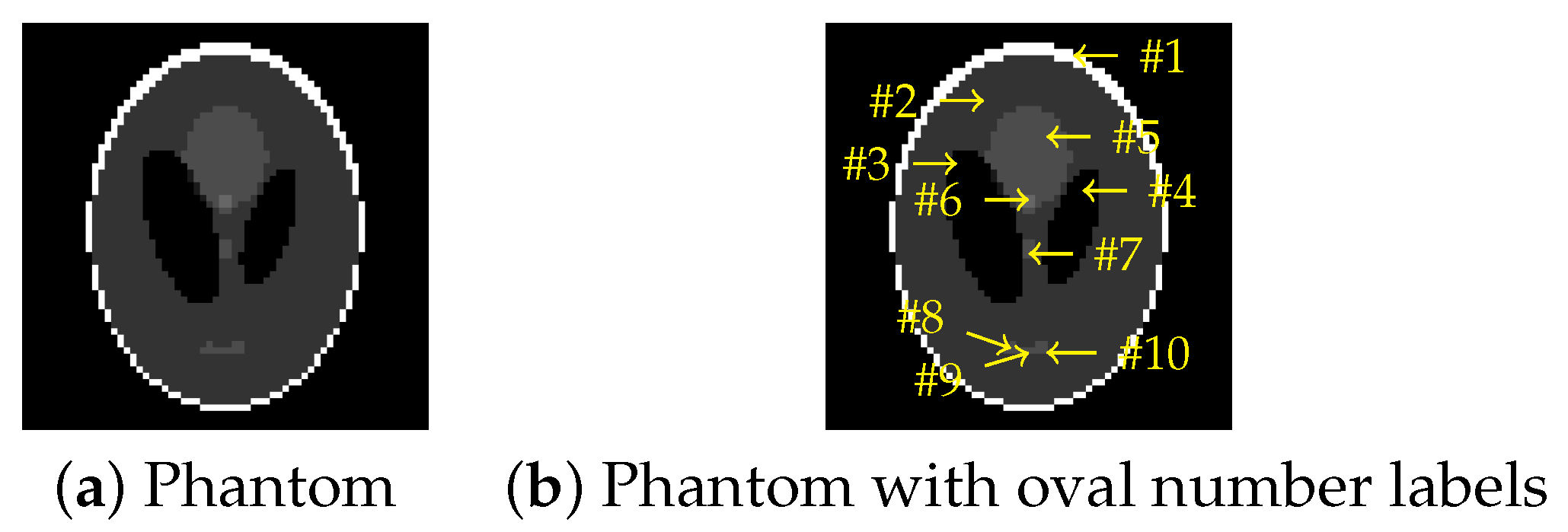
Figure 1. Structure of the whole network Θ .
Algorithms 16 00060 g001
Figure 2. Structure of the optimizee Ω .
Algorithms 16 00060 g002
Figure 3. Structure of block p.
Algorithms 16 00060 g003
Figure 4. Base phantom.
Algorithms 16 00060 g004
Figure 5. Histogram of projection SNRs in input data set.
Algorithms 16 00060 g005
Figure 6. Samples of learning data.
Algorithms 16 00060 g006
Figure 7. Structure of optimizer Λ . Dense ( n , f ) indicates a dense layer with n nodes and activation function f : R n R n . DropOut ( r ) indicates the dropout layer with dropout rate r. ReLU is short for rectified linear unit function.
Algorithms 16 00060 g007
Figure 8. Learning curve. Blue and red points are results for training data and validation data, respectively.
Algorithms 16 00060 g008
Figure 9. Dataset for testing.
Algorithms 16 00060 g009
Figure 10. Evaluation function values of z ( k ) with projection y for any k. Blue and red points are for parameters λ = λ ^ and ( 1 , 1 ) , respectively.
Algorithms 16 00060 g010aAlgorithms 16 00060 g010b
Figure 11. Contour map of evaluation function values D ( , z ( K ) ) with projection y for parameters γ , α . Blue and red points indicate λ ^ and ( 1 , 1 ) corresponding to the MLEM algorithm, respectively.
Algorithms 16 00060 g011
Figure 12. Phantom images of (a) e 6 , e 9 , and e 10 , (b) e 7 , and (c) e 8 for testing.
Algorithms 16 00060 g012
Figure 13. Evaluation function values of z ( k ) with projection y for any k. Blue and red points are for parameters λ = λ ^ 5 and ( 1 , 1 ) , respectively.
Algorithms 16 00060 g013
Figure 14. Contour map of evaluation function values D ( , z ( K ) ) with projection y for parameters γ , α . Blue and red points indicate λ ^ 5 and ( 1 , 1 ) corresponding to the MLEM algorithm, respectively.
Algorithms 16 00060 g014
Figure 15. Images reconstructed from projection y 6 by using proposed method with parameter λ ^ 1 and the MLEM algorithm. Subtraction images display in the range from 0 to 0.3.
Algorithms 16 00060 g015
Figure 16. Images reconstructed from projection y 8 by using the proposed method with parameter λ ^ 3 and the MLEM algorithm. Subtraction images display in the range from 0 to 0.15.
Algorithms 16 00060 g016
Table 1. Deformation ratios from base phantom. Symbol * indicates that the deformation ratio for the attribute uses a common value for each oval in the same group. See Figure 4b for “oval numbers”.
GroupOval
Numbers
IntensityMinor Axis LengthMajor Axis LengthHorizontal
Position
Vertical
Position
Angle of Rotation
1#1, #2 ± 10 % ± 20 % * ± 15 % * ± 0 % ± 0 % ± 0 %
2#3, #4, #5 ± 30 % ± 30 % ± 20 % ± 25 % ± 25 % ± 20 %
3#6, #7 ± 30 % ± 50 % ± 50 % ± 50 % ± 50 % ± 50 %
4#8, #9, #10 ± 30 % * ± 25 % * ± 25 % * ± 20 % * ± 20 % * ± 50 %
Disclaimer/Publisher’s Note: The statements, opinions and data contained in all publications are solely those of the individual author(s) and contributor(s) and not of MDPI and/or the editor(s). MDPI and/or the editor(s) disclaim responsibility for any injury to people or property resulting from any ideas, methods, instructions or products referred to in the content.

