Tunnel Traffic Evolution during Capacity Drop Based on High-Resolution Vehicle Trajectory Data

Abstract

Capacity drop is the critical phenomenon that triggers traffic congestion, while traffic evolution is very complex during a capacity drop. This study applied the empirical vehicle trajectory data to explore the traffic characteristics during the capacity drop at the tunnel bottleneck section. We first construct a capacity drop analysis model using image processing technology to extract high-precision vehicle trajectories. We then analyze the characteristics of the evolution process of the capacity drop at the bottleneck area. The results show that the capacity drop is a dynamic evolution process from free flow to congested flow where traffic operation is distinct. The capacity drop shows the difference between congested flow and non-congested flow. The driving characteristics of drivers in the two states are also different. The influence of lane-changing behavior on the capacity drop is estimated. In the free flow state, the disturbance caused by lane-changing can be quickly eliminated. With the increase in vehicle numbers in the area, the frequent lane-changing behavior accumulates disturbance. When the disturbance reaches a certain degree, congestion will occur, and the vehicle’s speed will drop sharply, resulting in a capacity drop.

1. Introduction

With the acceleration of urbanization and the improvement of motorization level in urban traffic, urban tunnel bears increasing traffic pressure, which is the most common bottleneck type of urban traffic [1,2,3]. Unlike open ground traffic, urban tunnels have typical characteristics such as limited building space, exceptional driving environment, unique driving rules, and significant internal and external brightness differences. The maximum discharge flow measured downstream decreases immediately when a bottleneck is activated. This phenomenon is called “capacity drop”. Vehicles are more susceptible to interference from various factors and form an agglomeration effect of traffic flow disturbance, causing tunnel congestion and triggering the “capacity drop” phenomenon [4,5,6]. The actual vehicle flow rate of the tunnel is significantly lower than the standard capacity.

Previous research shows that capacity drop has attracted significant attention from researchers. Loop detector data are generally used to estimate the occurrence of the capacity drop to establish the prediction model. Some research used vehicle trajectory data from the simulation model for capacity drop analysis. In our study, the advancement is that we applied the empirical vehicle trajectory data extracted from cameras to explore the characteristics of the traffic during the capacity drop at the tunnel bottleneck section. We also explored the influence of lane-changing behaviors on the capacity drop with empirical vehicle trajectory data to establish the prediction model.

Nanjing Yingtian Street Tunnel, as one of the fast channels connecting Jiangbei New Area and the main urban area, also undertakes the significant demand of commuting across the river. On the monitoring video platform of the whole tunnel, high-precision vehicle trajectory data are obtained, and the characteristics of the data are statistically analyzed.

2. Literature Review

Researchers observed the phenomenon of the capacity drop in early studies. Initially, the concept of the “capacity drop” first appeared in the 1960s when Edie [7] and Greenberg [8] obtained two significantly different areas by drawing the flow–density point diagram of the Lincoln Tunnel in the United States. There are free flow and congested flow. It has a significant flow difference at the regional junction of two areas, the “capacity drop” phenomenon. Koshi draws the “reverse-λ” shape of the flow–density point diagram and the discontinuity of the change from free flow to congested flow to explain the capacity drop [9]. He believed that the driver in congested traffic flow is more inclined to have a more considerable car-following distance, but this comment lacks corresponding data support. The range of 5%-30% drop in the maximum discharge flow at the bottleneck has been widely observed, bringing excessive travel delays and safety concerns [10,11,12].

Previous research has investigated the cause of capacity drop using aggregated traffic data from loop detectors. Kerner proposed the “three-phase traffic” theory and the concept of “phase transition” [13,14,15] and believed that the “phase transition” process of traffic flow caused the “breakdown phenomenon” of a sudden decrease in vehicle speed, resulting in capacity drop. Studies have observed capacity drop in areas where lane changing often occurs, near weaving segments [16,17], merging [18,19,20], diverging [21], and lane-drop [22] bottlenecks. Some researchers found that the magnitude of the capacity drop is associated with the density [23,24], the demand of ramp flows [25], the speed at the bottleneck [26], and the number of lanes [27].

Recent studies explored the capacity drop from the human behavior perspective. Based on Newell’s hyperbolic theory [28], Yeo conducted statistical analysis by intercepting part of the vehicle trajectory data in Next Generation Simulation (NGSIM) [29]. He elaborated and explained the asymmetric driving behavior theory [30] and effectively connected the capacity drop phenomenon with this theory. It is believed that after experiencing congestion, drivers tend to adopt a more considerable headway distance during acceleration. The shock wave formed by the disturbance during the driving process has a more noticeable impact on capacity drop [31,32]. The macroscopic node model and kinematic wave theory are proposed to predict the causes of the capacity drop [33,34].

Some researchers believe that car-following behaviors are the cause of the capacity drop. For example, Jin established a behavior model of first-order capacity drop at the continuous bottleneck based on the Lighthill–Whitham–Richards (LWR) model [35,36], taking the limited acceleration of the vehicle as an additional constraint of the optimal model of traffic flow at the bottleneck. More recently, Chen et al. revealed that combining different acceleration rates and desired driving behavior speeds induced voids and reduced capacity [37]. Through research and analysis of NGSIM data, Simon Oh quantified the traffic flow generated by stop-and-go waves and lane changing downstream of the bottleneck [38]. On the other hand, Zhang et al. considered the lane changer’s insertion speed as a factor in AIMSUM, a traffic simulation software. They found that lane-changing vehicles with a high insertion speed could offset the capacity drop [39].

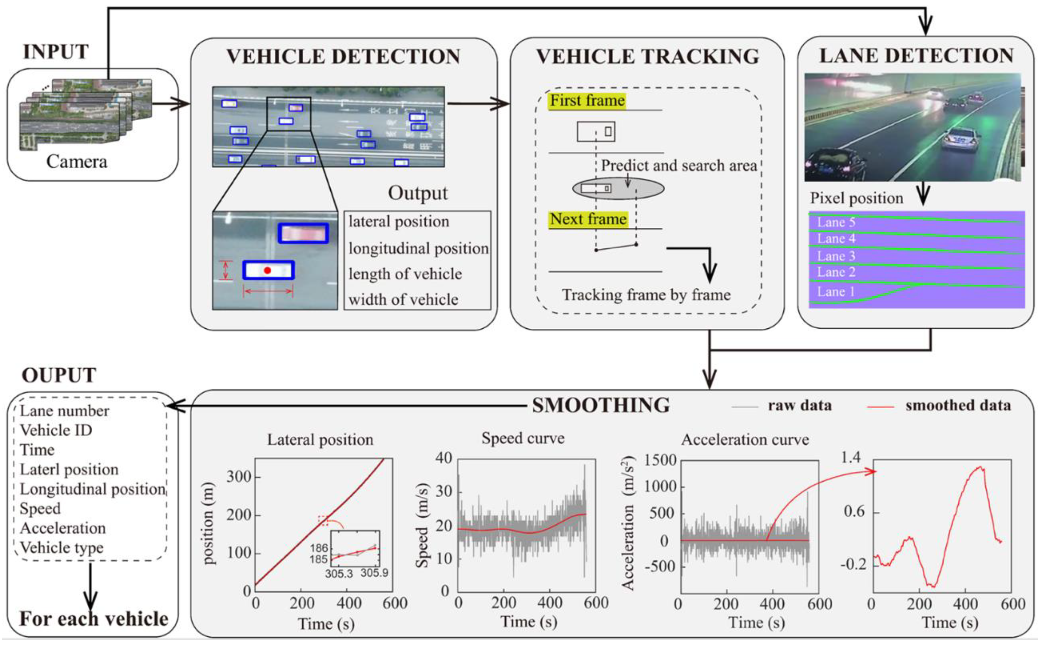
3. Tunnel Vehicle Trajectory Data Extraction

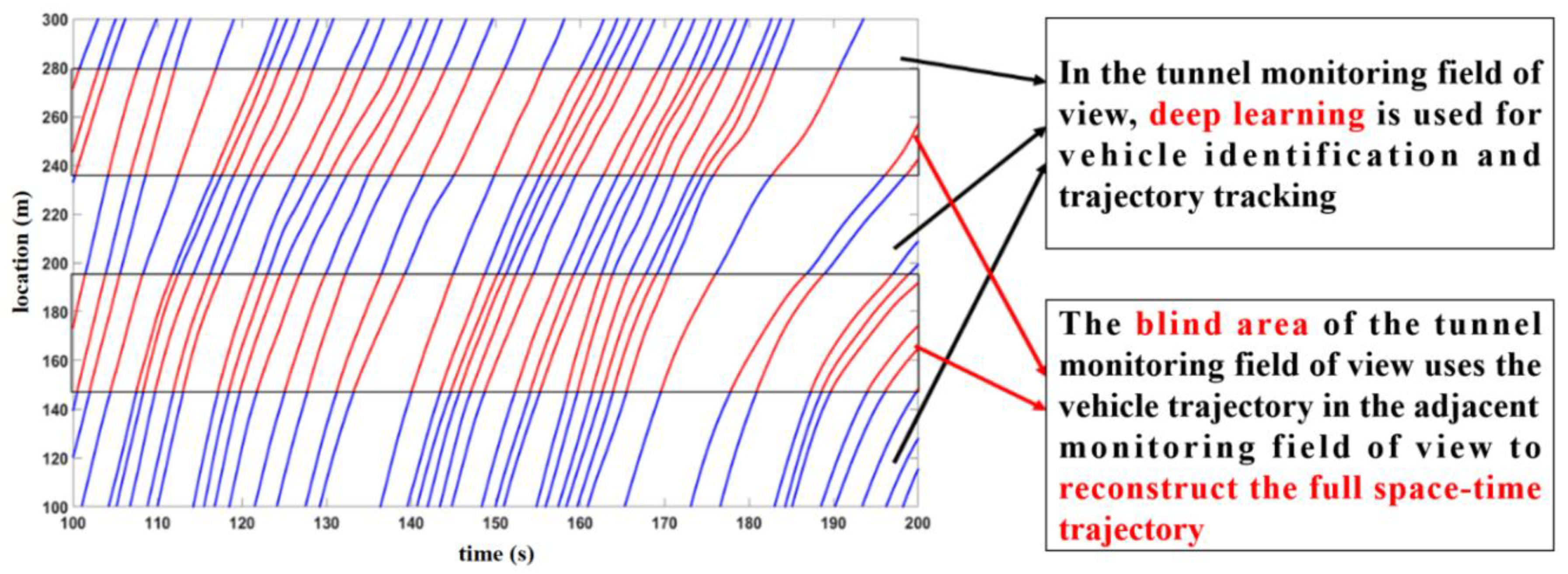
3.1. Extraction of Fixed-Point Vehicle Trajectory in the Tunnel

To obtain each vehicle’s spatial and temporal coordinate data in the tunnel monitoring field of view, it is necessary to identify and track each vehicle in the video. Firstly, each image frame is binarized, and the threshold value of vehicle identification size is set to realize each vehicle’s rough detection and identification. To further improve the accuracy and speed of detection, this paper adopts the emerging deep learning algorithm You Only Look Once (YOLO) v5 to recognize and detect moving targets in monitoring [40,41]. Then, the intermittent trajectory matching and missing trajectory completion are performed based on the speed limit judgment data association algorithm for the primary construction of vehicle trajectories. Then, the coordinate conversion method is applied to map the image coordinates to the Frenet coordinates along the lane and perpendicular to the direction of the lane. Finally, the overall algorithm of empirical mode decomposition (EMD) noise reduction is used to reduce the trajectory error and improve the trajectory accuracy at the fixed point of the tunnel [42].

3.2. Reconstruction of Vehicle Track in Entire Space–Time of Tunnel

There is a blind area of track detection of 40 to 70 m between the adjacent video surveillance of the tunnel. To obtain the space–time continuous track of vehicles in tunnels and ensure the track’s authenticity, the curves represent the track of the vehicle movement, which is improved based on the cubic Hermite interpolation method. The cubic polynomial function is introduced into the Hermite interpolation algorithm to solve the slope. This method does not need other vehicle motion information, the algorithm complexity is low, and the interpolation accuracy is higher than linear interpolation, cubic spline interpolation, and cubic Hermite interpolation. The overall schematic diagram is shown in Figure 1.

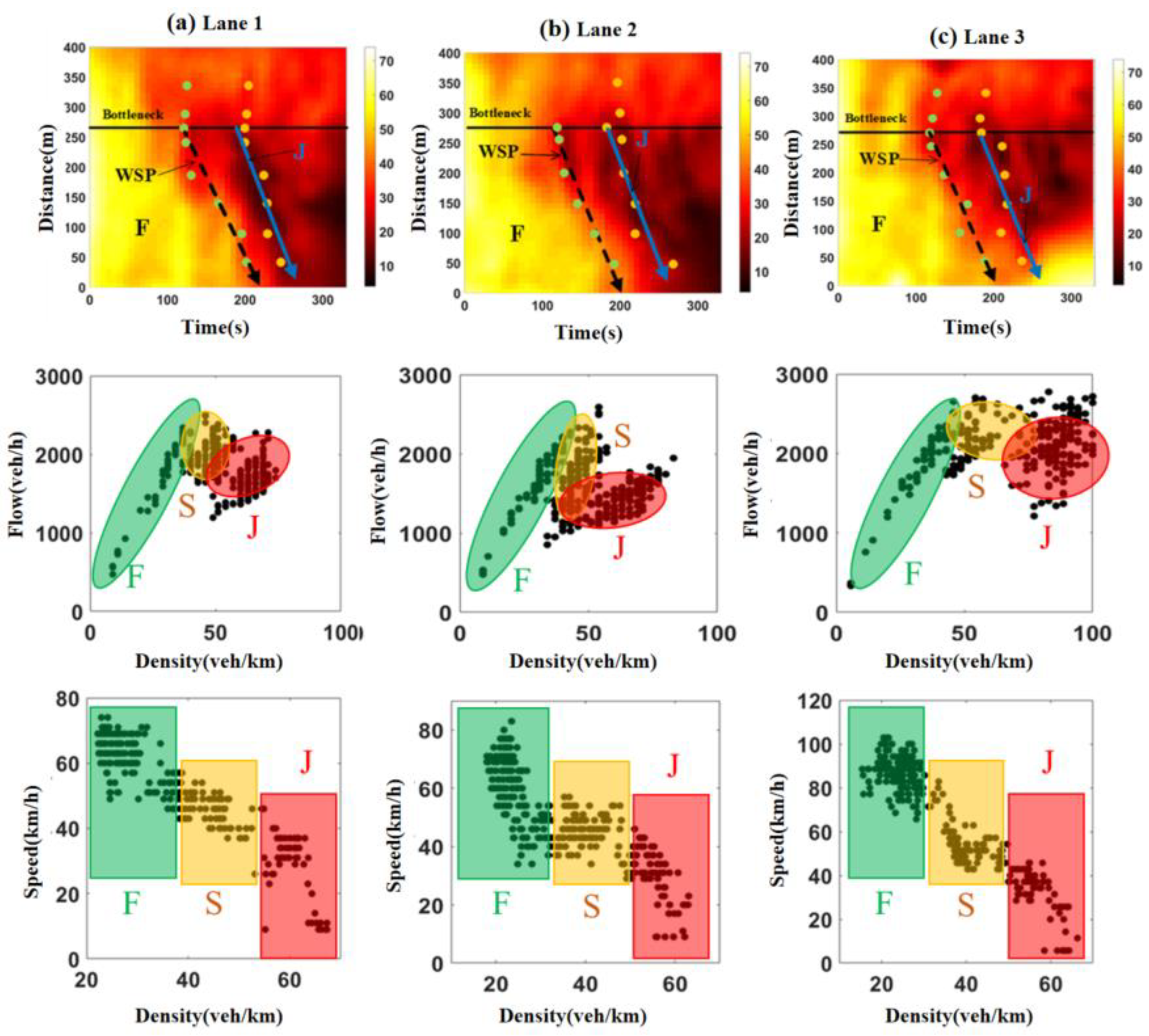
4. Analysis of Capacity Drop Based on Phase Transition-Theory

The capacity drop indicates the difference in capacity between the crowded and non-crowded flow. Many studies have taken the occurrence of congestion, queuing, and other phenomena as the prerequisites for the capacity drop. In this section, the inclined cumulative curve is used to identify the moment of traffic capacity drop at each section of the tunnel. Combined with Kerner’s three-phase traffic flow theory, the temporal and spatial characteristics of vehicle speed are used as indicators to draw the temporal and spatial characteristics of the vehicle track in each lane. The phase change points in vehicle track data are extracted in combination with various phase characteristics to study the correlation of traffic capacity drop.

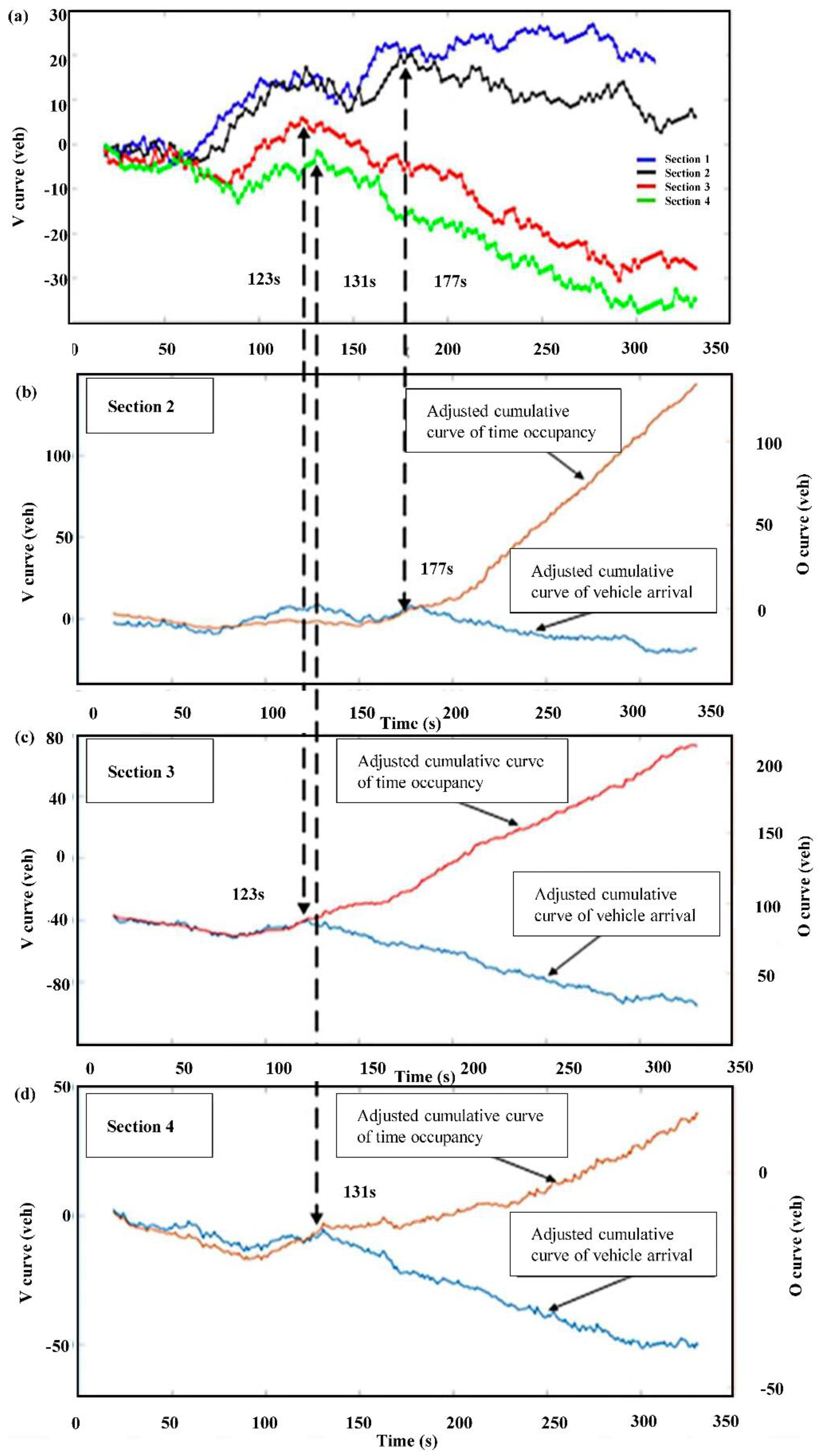
4.1. Identification of Tunnel Capacity Drop

The advantage of the vehicle oblique accumulation curve is that it can highlight the phase characteristics of the flow change at the section to identify the flow change point. However, the abrupt flow is not always the phenomenon of capacity drop. It is not enough to identify the moment of the capacity drop with the inclined cumulative curve of vehicles. By combining the inclined cumulative curve of time occupancy and recognizing the changing trend of a vehicle passing time at the section, the moment of the capacity drop can be more accurately determined. We draw the cumulative vehicle curve and the cumulative curve of time occupancy in the oblique coordinate system by combining the bottleneck characteristics and state parameters. Then, we enlarge the traffic change characteristics at the section to determine the moment of traffic capacity drop. The basic principle of the oblique accumulation curve is as follows:

Based on the original cumulative curve of the section, a background value is subtracted. The change characteristics of the curve are visually enlarged, and the change points of vehicle arrival intensity and vehicle delay at the section are identified. The curve formula is as follows:

$$\begin{array}{c}V\left(x,t\right)=N\left(x,t\right)-q_o\left(x\right)·t\\ O\left(x,t\right)=T\left(x,t\right)-t_o\left(x\right)·t\end{array}$$

where:

V$\left(x,t\right)$—the cumulative number of arrivals of vehicles passing through section x within t after adjustment;

$O\left(x,t\right)$—the cumulative curve of the time occupancy rate of vehicles passing through section x within t after adjustment;

$N\left(x,t\right)$—the cumulative number of arrivals of vehicles passing through section x within t;

$T\left(x,t\right)$—the cumulative curve of the time occupancy rate of vehicles passing through section x within t;

$q_o\left(x\right)$—background flow at section x, usually the maximum capacity at this section;

$t_o\left(x\right)$—undetermined parameter at section x, unit s/h.

Based on the construction method of the oblique cumulative curve of the appealing vehicle and combined with the research division of this area in this paper, the oblique cumulative curve of the critical sections (tunnel entrance and exit, slope change points, etc.), in the whole region of the tunnel is constructed. The oblique cumulative curves display “virtual departures,” such that the vertical displacements between any two are the excess vehicle accumulations (queueing) on the intervening tunnel segment. With the oblique coordinate system, each curve displays the quantity, the virtual vehicle counts to time, minus a background reduction. We conducted the adjustment tests for the background parameters of each section. The original parameter value is the average flow multiplied by the interval extending from the curves’ start time to the current time. Then, we tested the parameters varying from −10% to 10% of the original value for final use. After several adjustment tests, the background parameters of each section are determined to significantly enhance the visual effect of the flow rate change of sections.

In Figure 2, the oblique accumulation curves of vehicles at the four adjacent sections are all piecewise approximately linear, showing a stepped characteristic. As shown in the figure below, at 123 s, the traffic capacity first drops in the bottleneck section. Secondly, the traffic flow leaving the area downstream of the bottleneck is limited to the merge bottleneck and lags the merge bottleneck. At 131 s, the flow suddenly changes. At the same time, the congestion at the merge bottleneck gradually spreads to the segment at the upstream section. Further, at 177 s, the traffic capacity drops. By calculating the flow rate at the bottleneck section, the capacity before congestion formation is estimated to be 6700 veh/h, while the discharge flow after congestion formation is estimated to be 5850 veh/h. The magnitude of capacity drop at the merge bottleneck is 12.7%.

4.2. Analysis of Capacity Drop Based on Traffic Flow

This section uses vehicle speed’s temporal and spatial characteristics as reference indicators, and the three main lanes’ temporal and spatial trajectory diagrams are homogeneously abstracted. We then draw the three-phase traffic flow temporal and spatial characteristics of the main lanes (see Figure 3). Kerner’s empirical research shows that there are usually two main blocking patterns at a single bottleneck: the synchronized flow pattern (phase S) and the wide moving jam pattern (phase J). In Kerner’s theory, the phases J and S in congested traffic are observed outcomes in universal spatial–temporal features of real traffic data. Asynchronous flow appears at the bottleneck at the beginning of the congestion and propagates upstream of the bottleneck. The downstream front of the synchronized flow is often fixed at a bottleneck. In contrast, a wide-moving jam could occur spontaneously in this synchronous flow. A wide moving jam is meant to reflect the characteristic feature of the jam to propagate through any other state of traffic flow and any bottleneck while maintaining the velocity of the downstream jam front. The speed within the wide moving jam could be very low, and thus this pattern is also called stop-and-go traffic.

There is a connection between the capacity characteristic point and the phase change boundary of the three-phase traffic flow.

(1)

F->S: Free flow changes to synchronous flow. Traffic crash occurs with the spontaneous start and propagation of the synchronous flow (the upstream boundary of the synchronous flow propagates upstream, while the downstream boundary is fixed at the bottleneck). According to the black dotted arrow in the distance–time diagrams in the first row of subfigures in Figure 3, the vehicle begins to slow down when approaching the upstream interface, and the bottleneck capacity does not change significantly at this time.

(2)

S->J: Synchronous flow changes to jam flow. Some narrow moving jams (narrow moving jams) appeared in this state, and then they evolved into wide moving jams (J appeared). At this time, the capacity has been significantly reduced.

Combined with the characteristic points of capacity drop in the temporal and spatial diagram of the vehicle trajectory in the figure, it is found that the vehicle speed decreases significantly when the traffic flow is approaching the interface. It causes drivers to take a more considerable distance between vehicles, leading to the phenomenon of “traffic capacity drop” at the macro level. From the flow–density diagrams in the subfigures of Figure 3, it can be found that the traffic capacity drop points are all near the synchronous flow, and vehicles exhibit a significant speed reduction. The capacity decreased rapidly when the synchronous flow transitioned to the wide moving jam flow. In the synchronous flow state, the vehicle speed decreases while the density increases, and the traffic capacity does not change significantly. The synchronous flow is more like the accumulation process of disturbance. When the disturbance is sufficient, the jam flow occurs.

5. Analysis of Tunnel Driving Behavior

The capacity drop means that the traffic flow follows different operating rules in the two states of free flow and congested flow. The microscopic level is manifested as the characteristic difference of vehicle trajectory. When a certain percentage of drivers in the transportation system are affected by nearby driving vehicles, the traffic flow will lose stability, manifesting as congestion, traffic capacity drop, and other phenomena summarized as the “disturbance”. The significant source of disturbance in this study is the deceleration behavior of vehicles passing through the tunnel.

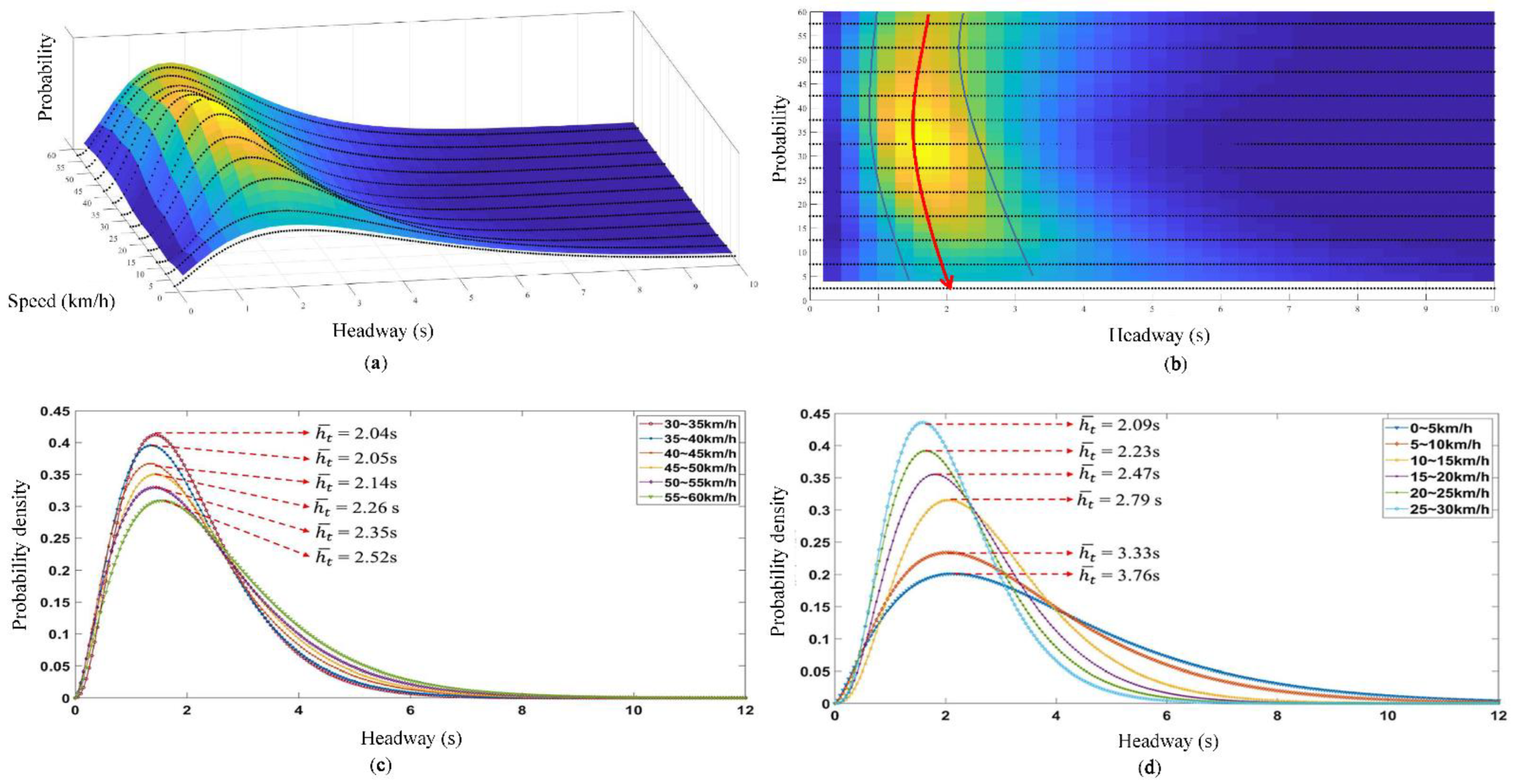
5.1. Analysis of Headway Distribution

The headway indicates the time difference between the two vehicles passing through the same position on the road and represents the maximum reaction time of the driver behind the vehicle when the current vehicle brakes suddenly. The headway distance is closely related to the traffic flow composition and driving behavior and is an essential indicator of road capacity, service level, and driving safety. The probability distribution of headway is shown in Figure 4.

The time headway for different driving speeds ranges from 2.04 s to 2.52 s in synchronous flow and from 2.09 s to 3.76 in the wide moving jam. The time headway distribution for the two traffic phases shows a clear difference. In synchronous flow, the disturbance caused by the lane-changing behavior forces the following vehicle to speed adaptation, varying from high speed to low speed. The traffic inflow at the bottleneck is similar to the extrusion process, and the headway distance is gradually compressed. Finally, the headway decreases slightly, explaining that the road system still maintains a high flow input in the synchronous flow state.

The traffic flow at the bottleneck has been compressed in the wide moving jam flow. The driver tends to drive at a higher distance for safety considerations in this state. In addition, the driver will have a certain psychological threshold of safe distance, even in a completely stationary state. There will still be a particular gap between vehicles, so it can be explained that in the state of wide moving jam flow, the distance between the fronts has been compressed because of the significantly reduced speed. The probability distribution of headway shows that the lower the speed, the larger the value.

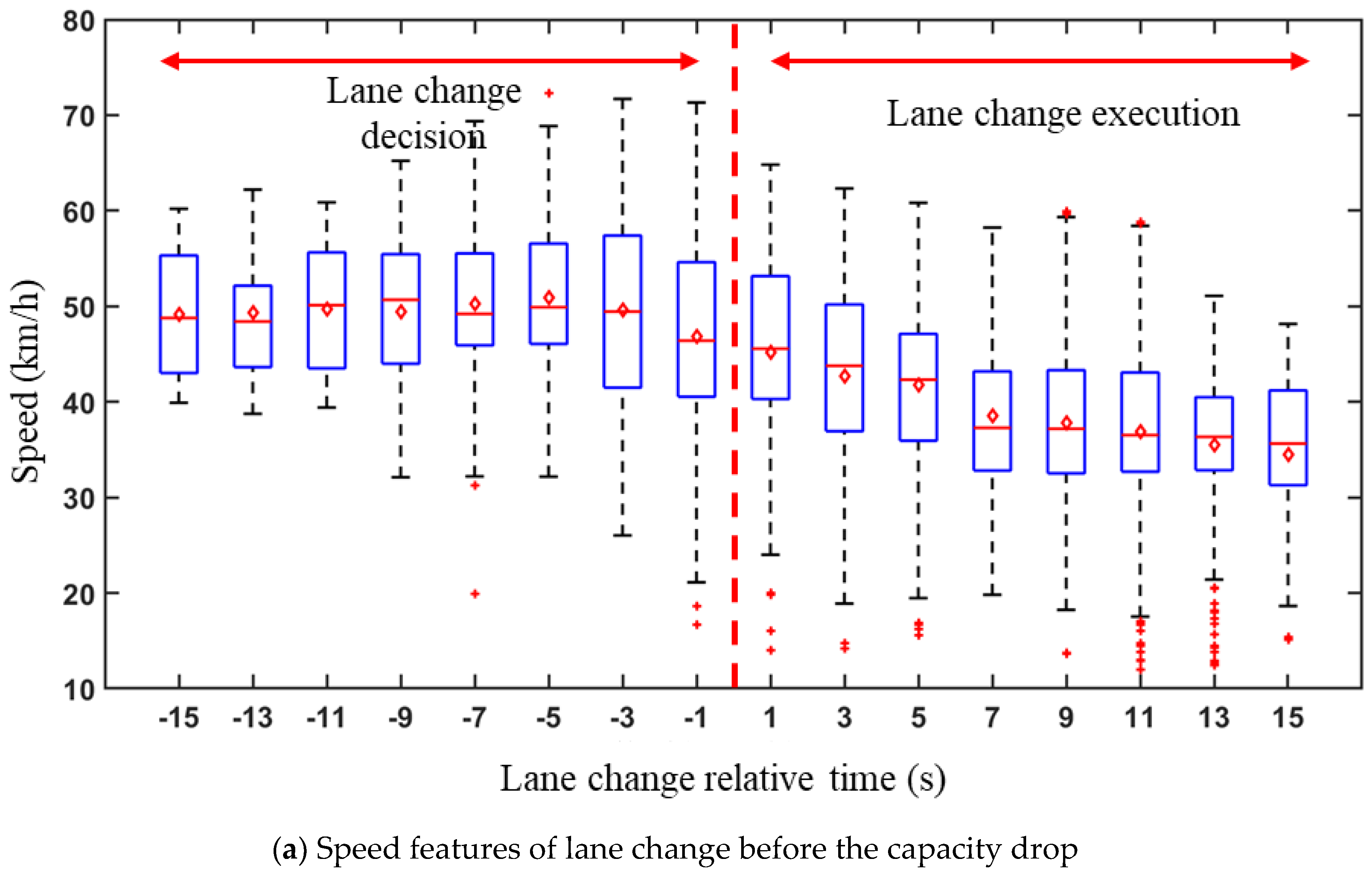
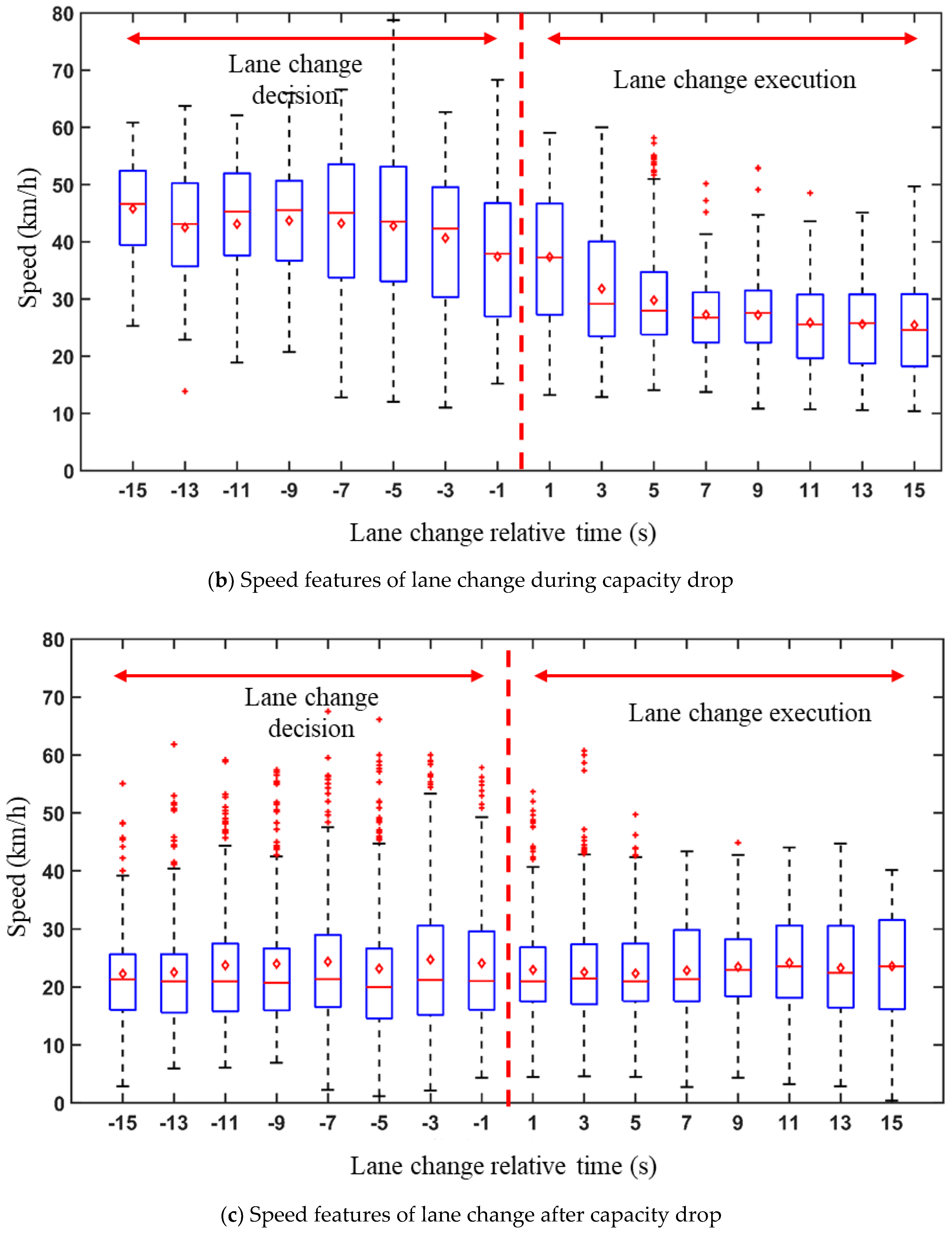
5.2. Analysis of Lane-Change Speed

The salient feature of a vehicle changing lanes is vehicle speed change. When the driver has an intention to change lanes, he usually takes a deceleration action, waits for the opportunity to enter the target lane, and adjusts his speed in the target lane to enter the stable following state of the target lane as soon as possible. Speed features of lane change vehicles are shown in Figure 5.

When the capacity decreases, the confluence bottleneck area is in a smooth state. When the driver intends to change lanes, he can quickly adjust his speed and complete the lane-changing behavior faster. At the same time, according to the trajectory characteristics of the previous chapter, the area runs at a higher speed and a more considerable distance. The lane-changing driver has complete space for speed adaptation in a short time and then changes lanes. As the upstream flow increases, the state of this area enters the synchronous flow phase. The deceleration behavior of the lane-changing driver in the original lane decision phase and the speed adjustment behavior in the execution phase cause the following vehicle to adapt to the speed. The disturbance to the following vehicle accumulates over time and ultimately causes the traffic capacity to decrease.

When the free flow of the study area changes to a congested flow, the lane-changing vehicles in the process of reduced capacity show a similar trend as before the reduced capacity. During this time, the speed exhibits large fluctuations and the fluctuating speed of the vehicle during the lane change. The following vehicles cause more significant disturbances, causing the drivers of the following vehicles to vacate a more substantial gap for safety reasons, thus causing a decrease in traffic capacity.

After the traffic capacity declines, the road shows more severe congestion, and lane-changing vehicles show a low-speed and stable trend. There are significant outliers in the speed box diagram at the lane-changing decision-making stage in this state. After inspection, these outliers are in the upstream input area or ramp, and the congestion state has not spread to this area.

We further calculate the speed change of vehicles on the target lane and original lane. The speed change rate a_i is the change of vehicle i’s speed after and before the lane change divided by the original speed. A positive rate indicates that the speed increases after the lane change and vice versa. The results on different lanes are summarized in

Table 1. Speed change of vehicles on different travel lanes.

	Lane 1		Lane 2		Lane 3		Lane 4
	Sample Size	Mean (S.D.)	Sample Size	Mean (S.D.)	Sample Size	Mean (S.D.)	Sample Size	Mean (S.D.)
aLC	34	0.042 (11.2)	100	−0.103 (0.400)	125	−0.098 (0.501)	259	−0.083 (0.451)
aFO	11	0.101 (0.221)	42	−0.014 (0.241)	50	0.153 (0.371)	103	0.079 (0.267)
aFT	17	−0.002 (0.283)	49	−0.057 (0.332)	69	−0.060 (0.328)	135	−0.052 (0.294)

a_LC is the speed change rate of the lane change vehicle, a_FO is the speed change rate of the following vehicle on the original lane, and a_FT is the speed change rate of the following vehicle on the target lane.

. For lane-changing vehicles and following vehicles on the target lane, the speed of most vehicles is reduced during the lane-changing process. The lane-changing vehicle in the outer lane has a more serious speed reduction. When the vehicle changes lanes to the inner lane, its speed increases. The main reason is that the inner lane runs relatively smoothly with less disturbance. The driver of a lane-changing vehicle can better adjust its driving state after entering the inner lane because the speed has increased. For the following vehicle on the original lane, the standard deviation of the parameter is relatively small during the lane change, which means that the original lane is less disturbed, and the speed fluctuation reflected is less.

6. Conclusions and Discussion

This paper constructs the capacity drop analysis using video image processing technology to extract high-precision vehicle trajectory data. The article analyzes the characteristics of the evolution process of traffic congestion at the bottleneck in a tunnel section. The capacity drop is captured by plotting the cumulative vehicle count curves. The capacity at the merge bottleneck is found to be 6700 veh/h, while the magnitude of the capacity drop is estimated to be 12.7%. We also explored the driving characteristics related to the occurrence of the capacity drop. The results show that the time headway for different driving speeds ranges from 2.04 s to 2.52 s in synchronous flow and from 2.09 s to 3.76 in the wide moving jam, which indicates a clear difference between the two traffic phases.

Based on the analysis, the main findings are summarized as follows: (1) we captured the dynamic process of tunnel traffic capacity drop involving free flow and congested flow; (2) the capacity drop in the diagrams shows the difference between congested flow and non-congested flow, and deep analysis shows the different driving characteristics of drivers in the two states; (3) the influence of lane-changing behavior on the capacity drop is captured by analyzing the driving behaviors. In the free flow state, the disturbance caused by lane-changing can be quickly eliminated. With the increase in vehicle count, frequent lane-changing behavior will accumulate disturbance. When the disturbance reaches a certain degree, congestion will occur, and the speed of vehicles will drop sharply, resulting in a capacity drop. The study’s findings can provide evidence of explanations of causes of capacity in tunnel bottlenecks in urban areas, supporting real-time traffic control strategies to preserve tunnel capacity.

The algorithm proposed in the study has the potential for applications in engineering. For example, the traffic control center can use the algorithm to accurately monitor and predict traffic conditions. Once the capacity drop is captured or predicted, we can quickly inform the drivers about the upcoming congestions within the tunnel via roadside variable message signs or vehicle onboard displays to take some precautions. In addition, we can apply active traffic management (variable speed limit, ramp metering, lane control, etc.), techniques to prevent the drop in tunnel capacity further and maintain a high flow rate [43]. Finally, as we explored the vehicle driving behaviors that trigger the capacity drop, we can apply some vehicle behavior control measures (such as lane change regulations) to prevent the disturbance that causes capacity drop. Those are some efforts that can be conducted for engineering applications based on the algorithms in our research.

In our research, we investigated the vehicle driving behaviors that cause the capacity drop in tunnel traffic. The vehicle movements can be coordinated via the cooperative connected and automated mobility (CCAM) technique to prevent the occurrence of capacity drop and congestion. Cooperative connected and automated mobility (CCAM) aims to achieve a safer, more efficient, and more comfortable mobility mode by coordinating vehicle motion states with sharing information [44]. CCAM mainly includes the technology of vehicular communications, automated driving, and cooperating transportation systems. Recently, numerical research proposed a series of innovative technology for CCAM, such as 5G-SDN-MPTCP-based communication systems [45], multi-tier orchestration platform architectures [46], safety-related assessment platforms [47], and a significant number of cooperative adaptive cruising control algorithms [48,49]. There are also some evaluation and incentive systems related to the social and economic benefits of CCAM.

State-of-the-art CCAM has been applied in practices in Europe, America, and Asia. For example, Europe conducted a project named H2020 5GCroCo to define a successful path toward providing CCAM services along with cross-border scenarios and reduce the uncertainties of an actual 5G cross-border deployment [50]. A Plan for Europe is conducted to achieve 5G deployment along the main transport corridors for autonomous vehicles in European Union [51]. America has carried out a series of travel services by connected and automated vehicles, such as MILO in Texas, ARIBO in North Carolina, AAA, and Nevada [52].

Our research found that the disturbance caused by lane changes, especially when the disturbance reaches a certain degree, significantly impacts traffic stability and capacity drop. Thus, we can coordinate and control the vehicle lane change moment via the CCAM, to control the cumulative disturbance under the critical threshold. The proposed algorithm can help identify this threshold by analyzing the traffic flow and vehicle trajectory samples. Additionally, the algorithm should be slightly updated to identify more driving parameters for the CCAM system, such as headway, the gap for a lane change, acceleration/deceleration rate, etc.

References

1. Jin, W.-L. Kinematic wave models of sag and tunnel bottlenecks. Transp. Res. Part B Methodol. 2018, 107, 41–56. [Google Scholar] [CrossRef]
2. Sun, J.; Li, T.; Yu, M.; Zhang, H.M. Exploring the Congestion Pattern at Long-Queued Tunnel Sag and Increasing the Efficiency by Control. IEEE Trans. Intell. Transp. Syst. 2018, 19, 3765–3774. [Google Scholar] [CrossRef]
3. Anderson, M.L.; Davis, L.W. An empirical test of hypercongestion in highway bottlenecks. J. Public Econ. 2020, 187, 104197. [Google Scholar] [CrossRef]
4. Wada, K.; Martinez, I.; Jin, W.-L. Continuum car-following model of capacity drop at sag and tunnel bottlenecks. Transp. Res. Part C Emerg. Technol. 2020, 113, 260–276. [Google Scholar] [CrossRef]
5. Martínez, I.; Jin, W.-L. Impact of VSL Location on Capacity Drop: A Case of Sag and Tunnel Bottlenecks. Transp. Res. Procedia 2018, 34, 12–19. [Google Scholar] [CrossRef]
6. Wang, Y.; Yu, X.; Zhang, S.; Zheng, P.; Guo, J.; Zhang, L.; Hu, S.; Cheng, S.; Wei, H. Freeway traffic control in presence of capacity drop. IEEE Trans. Intell. Transp. Syst. 2020, 22, 1497–1516. [Google Scholar] [CrossRef]
7. Edie, L.C. Car-Following and Steady-State Theory for Noncongested Traffic. Oper. Res. 1961, 9, 66–76. [Google Scholar] [CrossRef]
8. Greenberg, H. An Analysis of Traffic Flow. Oper. Res. 1959, 7, 79–85. [Google Scholar] [CrossRef]
9. Koshi, M. Some findings and an overview on vehicular flow characteristics. In Proceedings of the 8th International Symposium on Transportation and Traffic Theory, Toronto, ON, Canada, 1 January 1983. [Google Scholar]
10. Banks, J.H. The two-capacity phenomenon: Some theoretical issues. Transp. Res. Rec. 1991, 1320, 234–241. [Google Scholar]
11. Kim, K.; Cassidy, M.J. A capacity-increasing mechanism in freeway traffic. Transp. Res. Part B Methodol. 2012, 46, 1260–1272. [Google Scholar] [CrossRef]
12. Cassidy, M.J. An Empirical and Theoretical Study of Freeway Weave Bottlenecks. 2009. Available online: https://escholarship.org/uc/item/2970816w (accessed on 10 September 2021).
13. Kerner, B.S. Experimental Features of Self-Organization in Traffic Flow. Phys. Rev. Lett. 1998, 81, 3797–3800. [Google Scholar] [CrossRef]
14. Kerner, B.S.; Rehborn, H. Experimental properties of complexity in traffic flow. Phys. Rev. E 1996, 53, R4275–R4278. [Google Scholar] [CrossRef]
15. Kerner, B.S. Three-phase traffic theory and highway capacity. Phys. A Stat. Mech. Its Appl. 2002, 333, 379–440. [Google Scholar] [CrossRef] [Green Version]
16. Instability in Dense Highway Traffic: A Review. In Proceedings of the Second International Symposium on the Theory of Traffic Flow, London, UK; Organisation for Economic Co-Operation and Development: Paris, France, 1963; pp. 73–83.
17. Marczak, F.; Daamen, W.; Buisson, C. Empirical Analysis of Lane Changing Behavior at a Freeway Weaving Section. In Proceedings of the 93th Annual Meeting of the TRB, Washington, DC, USA, 12–16 January 2014. [Google Scholar]
18. Liu, W.; Chen, K.Q.; Tian, Z.Z.; Yang, G.C. Capacity of Urban Arterial Weaving Sections under Lane Signal Control Strategy. Transp. Res. Rec. J. Transp. Res. Board 2019, 2673, 69–77. [Google Scholar] [CrossRef]
19. Cassidy, M.J.; Ahn, S. Driver turn-taking behavior in congested freeway merges. Transp. Res. Rec. 2005, 1934, 140–147. [Google Scholar] [CrossRef]
20. Cassidy, M.J.; Rudjanakanoknad, J. Increasing the capacity of an isolated merge by metering its on-ramp. Transp. Res. Part B Methodol. 2005, 39, 896–913. [Google Scholar] [CrossRef] [Green Version]
21. Chen, D.; Ahn, S. Capacity-drop at extended bottlenecks: Merge, diverge, and weave. Transp. Res. Part B Methodol. 2018, 108, 1–20. [Google Scholar] [CrossRef]
22. Zhou, Y.; Chung, E.; Cholette, M.E.; Bhaskar, A. Real-Time Joint Estimation of Traffic States and Parameters Using Cell Transmission Model and Considering Capacity Drop. In Proceedings of the 21st IEEE Conference on Intelligent Transportation Systems, Maui, HI, USA, 4–7 November 2018; pp. 2797–2804. [Google Scholar] [CrossRef]
23. Chung, K.; Rudjanakanoknad, J.; Cassidy, M.J. Relation between traffic density and capacity drop at three freeway bottlenecks. Transp. Res. Part B Methodol. 2007, 41, 82–95. [Google Scholar] [CrossRef]
24. Lu, Y.; Wong, S.; Zhang, M.; Shu, C.-W.; Chen, W. Explicit construction of entropy solutions for the Lighthill–Whitham–Richards traffic flow model with a piecewise quadratic flow–density relationship. Transp. Res. Part B Methodol. 2008, 42, 355–372. [Google Scholar] [CrossRef]
25. Srivastava, A.; Geroliminis, N. Empirical observations of capacity drop in freeway merges with ramp control and integration in a first-order model. Transp. Res. Part C Emerg. Technol. 2013, 30, 161–177. [Google Scholar] [CrossRef] [Green Version]
26. Parzani, C.; Buisson, C. Second-Order Model and Capacity Drop at Merge. Transp. Res. Rec. J. Transp. Res. Board 2012, 2315, 25–34. [Google Scholar] [CrossRef]
27. Oh, S.; Yeo, H. Estimation of Capacity Drop in Highway Merging Sections. Transp. Res. Rec. J. Transp. Res. Board 2012, 2286, 111–121. [Google Scholar] [CrossRef]
28. Bick, J.H.; Newell, G.F. A continuum model for two-directional traffic flow. Q. Appl. Math. 1960, 18, 191–204. [Google Scholar] [CrossRef] [Green Version]
29. Yeo, H. A proposed asymmetric microscopic traffic flow theory. In Proceedings of the 88th Transportation Research Board Annual Meeting, Washington, DC, USA, 15 November 2009. [Google Scholar]
30. Yeo, H.; Skabardonis, A.; Halkias, J.; Colyar, J.; Alexiadis, V. Oversaturated freeway flow algorithm for use in next generation simulation. Transp. Res. Rec. 2008, 2088, 68–79. [Google Scholar] [CrossRef]
31. Calvert, S.C.; van Wageningen-Kessels, F.L.M.; Hoogendoorn, S.P. Capacity drop through reaction times in heterogeneous traffic. J. Traffic Transp. Eng. 2018, 5, 96–104. [Google Scholar] [CrossRef]
32. Yuan, K.; Knoop, V.L.; Leclercq, L.; Hoogendoorn, S.P. Capacity drop: A comparison between stop-and-go wave and standing queue at lane-drop bottleneck. Transp. B Transp. Dyn. 2017, 5, 145–158. [Google Scholar] [CrossRef] [Green Version]
33. Jin, W.-L.; Gan, Q.-J.; Lebacque, J.-P. A kinematic wave theory of capacity drop. Transp. Res. Part B Methodol. 2015, 81, 316–329. [Google Scholar] [CrossRef] [Green Version]
34. Monamy, T.; Haj-Salem, S.; Lebacque, J.-P. A macroscopic node model related to capacity drop. Procedia Soc. Behav. Sci. 2012, 54, 1388–1396. [Google Scholar] [CrossRef] [Green Version]
35. Jin, W.-L. A first-order behavioral model of capacity drop. Transp. Res. Part B Methodol. 2017, 105, 438–457. [Google Scholar] [CrossRef]
36. Leclercq, L.; Laval, L.A.; Chiabaut, N. Capacity drops at merges: An endogenous model. Transp. Res. Part B Methodol. 2011, 45, 1302–1313. [Google Scholar] [CrossRef]
37. Chen, D.J.; Sivastava, A.; Ahn, S.; Li, T. Traffic dynamics under speed disturbance in mixed traffic with automated and non-automated vehicles. Transp. Res. Part C 2019, 38, 709–729. [Google Scholar] [CrossRef]
38. Oh, S.; Yeo, H. Impact of stop-and-go waves and lane changes on discharge rate in recovery flow. Transp. Res. Part B Methodol. 2015, 77, 88–102. [Google Scholar] [CrossRef]
39. Zhang, C.; Sabar, N.; Chung, E.; Bhaskar, A.; Guo, X. Optimisation of lane-changing advisory at the motorway lane drop bottleneck. Transp. Res. Part C Emerg. Technol. 2019, 106, 303–316. [Google Scholar] [CrossRef]
40. Rahman, R.; Bin Azad, Z.; Hasan, B. Densely-Populated Traffic Detection Using YOLOv5 and Non-maximum Suppression Ensembling. In Proceedings of the International Conference on Big Data, IoT, and Machine Learning 2022, Sydney, Australia, 22–23 October 2022; Springer: Singapore, 2022; pp. 567–578. [Google Scholar] [CrossRef]
41. Ke, R.; Li, Z.; Tang, J.; Pan, Z.; Wang, Y. Real-Time Traffic Flow Parameter Estimation From UAV Video Based on Ensemble Classifier and Optical Flow. IEEE Trans. Intell. Transp. Syst. 2018, 20, 54–64. [Google Scholar] [CrossRef]
42. Chen, X.; Li, Z.; Yang, Y.; Qi, L.; Ke, R. High-Resolution Vehicle Trajectory Extraction and Denoising From Aerial Videos. IEEE Trans. Intell. Transp. Syst. 2020, 22, 3190–3202. [Google Scholar] [CrossRef]
43. Fuhs, C.; Parsons, B. Synthesis of Active Traffic Management Experiences in Europe and the United States; No. FHWA-HOP-10-031; Federal Highway Administration: Washington, DC, USA, 2010.
44. Ferreira, J. Cooperative, Connected and Automated Mobility (CCAM): Technologies and Applications. Electronics 2019, 8, 1549. [Google Scholar] [CrossRef] [Green Version]
45. Slamnik-Krijestorac, N.; Yilma, G.M.; Liebsch, M.; Yousaf, F.Z.; Marquez-Barja, J. Collaborative orchestration of multi-domain edges from a Connected, Cooperative and Automated Mobility (CCAM) perspective. IEEE Trans. Mob. Comput. 2021, 1. [Google Scholar] [CrossRef]
46. Centenaro, M.; Berlato, S.; Carbone, R.; Burzio, G.; Cordella, G.F.; Riggio, R.; Ranise, S. Safety-Related Cooperative, Connected, and Automated Mobility Services: Interplay Between Functional and Security Requirements. IEEE Veh. Technol. Mag. 2021, 16, 78–88. [Google Scholar] [CrossRef]
47. Sawant, J.; Chaskar, U.; Ginoya, D. Robust Control of Cooperative Adaptive Cruise Control in the Absence of Information About Preceding Vehicle Acceleration. IEEE Trans. Intell. Transp. Syst. 2021, 99, 5589–5598. [Google Scholar] [CrossRef]
48. Cui, L.; Chen, Z.; Wang, A.; Hu, J.; Park, B.B. Development of a Robust Cooperative Adaptive Cruise Control With Dynamic Topology. IEEE Trans. Intell. Transp. Syst. 2022, 23, 4279–4290. [Google Scholar] [CrossRef]
49. Alonso Raposo, M.; Grosso, M.; Després, J.; Fernández Macías, E.; Galassi, C.; Krasenbrink, A.; Krause, J.; Levati, L.; Mourtzouchou, A.; Saveyn, B.; et al. An Analysis of Possible Socio-Economic Effects of a Cooperative, Connected and Automated Mobility (CCAM) in Europe; Technical Report; Publications Office of the European Union: Luxembourg, 2018; pp. 1–212. Available online: https://core.ac.uk/download/pdf/157830385.pdf (accessed on 15 January 2022).
50. Munoz, R.; Vazquez-Gallego, F.; Casellas, R.; Vilalta, R.; Sedar, R.; Alemany, P.; Martinez, R.; Alonso-Zarate, J.; Papageorgiou, A.; Catalan-Cid, M.; et al. 5GCroCo Barcelona Trial Site for Cross-border Anticipated Cooperative Collision Avoidance. In Proceedings of the 2020 European Conference on Networks and Communications (EuCNC), Dubrovnik, Croatia, 15–18 June 2020. [Google Scholar]
51. Lemstra, W. Leadership with 5G in Europe: Two contrasting images of the future, with policy and regulatory implications. Telecommun. Policy 2018, 42, 587–611. [Google Scholar] [CrossRef]
52. Qu, G.; Qiu, B.; Zhang, Y.; Wang, H. The Industry Situation and Inspiration of Intelligent Connected Vehicles in Europe, America and Japan. Cyber Secur. Intell. Anal. 2021, 1342, 259–265. [Google Scholar] [CrossRef]
Figure 1. Schematic diagram of extraction steps of space–time trajectory.
Algorithms 15 00240 g001aAlgorithms 15 00240 g001b
Figure 2. Confirmation of traffic capacity drop time of each tunnel section.
Algorithms 15 00240 g002
Figure 3. Analysis of tunnel capacity drop based on three-phase traffic flow.
Algorithms 15 00240 g003
Figure 4. Probability distribution of headway. (a) Probability fitting diagram of speed-headway distribution in 3D, (b) Probability fitting diagram of speed-headway distribution in 2D, (c) Schematic diagram of the headway probability distribution fitting in the synchronous flow state, (d) Schematic diagram of the headway probability distribution fitting in the blocked flow state.
Algorithms 15 00240 g004
Figure 5. Speed features of lane change vehicles.
Algorithms 15 00240 g005aAlgorithms 15 00240 g005b