Domain Generalization Model of Deep Convolutional Networks Based on SAND-Mask

Abstract

In the actual operation of the machine, due to a large number of operating conditions and a wide range of operating conditions, the data under many operating conditions cannot be obtained. However, the different data distributions between different operating conditions will reduce the performance of fault diagnosis. Currently, most studies remain on the level of generalization caused by a change of working conditions under a single condition. In the scenario where various conditions such as speed, load and temperature lead to changes in working conditions, there are problems such as the explosion of working conditions and complex data distribution. Compared with previous research work, this is more difficult to generalize. To cope with this problem, this paper improves generalization method SAND-Mask (Smoothed-AND (SAND)-masking) by using the total gradient variance of samples in a batch instead of the gradient variance of each sample to calculate parameter σ. The SAND-Mask method is extended to the fault diagnosis domain, and the DCNG model (Deep Convolutional Network Generalization) is proposed. Finally, multi-angle experiments were conducted on three publicly available bearing datasets, and diagnostic performances of more than 90%, 99%, and 70% were achieved on all transfer tasks. The results show that the DCNG model has better stability as well as diagnostic performance compared to other generalization methods.

1. Introduction

In the industrial production of the actual scene, the machine ran 24 h a day, usually for the real-time monitoring of running status of the machine, and it is very important to guarantee that the normal operation of machine fault diagnosis is able to build machine operation data and the relationships between the running state for real-time monitoring of the running status of the machine, as these have important research value. Generally, training data and test data are assumed to have the same distribution in fault diagnosis. However, due to the unavailability of some working condition data and the different distributions of data in different working conditions, fault diagnosis in an unknown working condition with data that pose a challenge to existing fault diagnosis methods.

Guo [1] proposed an RNN-based health indicator HI (health indicator) by extracting features and then transferring them to RNN networks and calculating the health indicator HI to predict bearing RUL (Remaining Useful Life), and the effectiveness of this method was demonstrated by bearing experimental data. Pan [2] proposed a 1D-CNN combined with LSTM networks for a bearing diagnosis model, which was had the best classification accuracy that reached 99.6% without any preprocessing of the data. Jiang [3] proposed a deep recurrent neural network (DRNN) model, which consists of a stack of hidden units and a deep recurrent neural network. The model consists of stacked hidden units and LSTM units, and experiments show that classification accuracy can reach 94.75%. Zhang [4] constructed a fault diagnosis model by combining a ResNet model, which directly analyzes and diagnoses raw unprocessed data, and experiments show that, compared with CNN, Zhao [5] used wavelet coefficients to improve diagnosis accuracy in order to improve the performance of the ResNet-based diagnostic model by weighing the wavelet coefficients on a planetary gearbox containing severe noise; this had higher accuracy compared to other deep learning algorithms.

The data-driven deep learning fault diagnosis approach based on data makes the assumption that training data are equally distributed with test data, which is usually not valid in practical scenarios. The domain adaptive DA (Domain Adaptation) technique and domain generalization DG (Domain Generalization) technique in migration learning are the two most important methods for solving the domain offset problem, which has been used by research scholars in the field of fault diagnosis to solve the domain offset problem caused by a change in working conditions in recent years. Domain offset fault diagnosis in migration learning is roughly divided into three broad scenarios: similar working conditions across machines, different working conditions across machines, and different working conditions of the same machine, and the first two cases are not discussed here. For the different working conditions of the same machine, Li [6] proposed a generalization model by using domain extension and distance measurement methods, which can learn generalized features from antagonistic heterogeneous domains, and verified the validity of the method on two rotating machinery datasets. Liao [7] proposed a deep semi-supervised domain comprehensive network for fault diagnosis of variable-speed rotating machinery, which can effectively extend the model to fault diagnosis tasks under invisible speed. Both of these studies are limited to the case of domain generalization caused by a single condition such as rotation speed, but in the actual scene, multiple conditions can cause changes in the same machine condition. At present, most research studies are conducted in a scenario using a single condition, leading to the change of working conditions, and the scenario of multiple conditions, leading to a change of working conditions that needs to be further explored:

• Its operating modes are numerous, and the characteristics of the working condition of the similarities and differences between the data are examined. The total gradient variance of all samples in the batch is used to replace the gradient variance of each sample to calculate parameter σ, which improves the generalization method of SAND-Mask [8] to calculate the gradient variance of network parameters, and extends SAND-Mask to the fault diagnosis scenario where multiple conditions lead to the change of working conditions.
• This paper proposes a new fault diagnosis DCNG generalization model. This model is suitable for the target domain data and it will not be able to access and change a variety of conditions, such as speed and load point, for more complex and difficult cases in order to generalize conditions resulting from a variety of conditions. In the open CWRU (Case Western Reserve University) data set and KAT (Konstruktions-und Antriebstechnik (KAT)) data set, a single condition led to a change of working conditions in MFPT—(Society for) Machinery Failure Prevention Technology). In an experimental comparison between the generalized model DCNG and the ungeneralized model, the experimental comparison between the generalized model DCNG and the model using other generalization measures in the image field, and the influence of different parameters on the generalized model DCNG in this paper show that the performance and stability of the generalized model in this paper are better than other models.

In the second section, this paper briefly describes previous studies on fault diagnosis to solve the domain offset problem and describes the network structure of the proposed DCNG model and the improvement of gradient variance in SAND-Mask calculation. Then, in the third section, the experiments of the DCNG model on three public data sets are analyzed. Finally, the DCNG model is discussed and the work of this paper is summarized in the fourth and fifth sections, respectively.

2. Materials and Methods

2.1. Related Work

In a real-world scenario, it would be impractical to gather sufficient tagging data and complete information about the condition of the machine due to the complexity of the machine and the impact of the production environment. In addition, the data distribution between different operating conditions of the machine is different, which leads to the problem of domain shifts and seriously reduces the performance of fault diagnosis. Currently, scholars and engineers try to use transfer learning to solve the above problems, which can be roughly divided into two categories: knowledge transfer between different machines and knowledge transfer from the same machine. Many meaningful research studies have been conducted on transferring the diagnostic knowledge of laboratory machine to actual machines, transferring diagnostic knowledge of one machine to a machine of the same type or different size and transferring diagnostic knowledge between different working conditions of the same machine, such as load and speed change.

Yang [9] proposed a features-based transfer neural network model for bearing fault diagnosis. By learning diagnosis knowledge from laboratory bearing data, a domain adaptive method was used to correct the differences between features so as to transfer diagnosis knowledge to actual scene bearings. Chen [10] proposed a cross-domain feature extraction method for bearing fault diagnosis by using the theory of transfer component analysis, and experiments verified the effectiveness of the method. Xie [11] applied the theory of transfer component analysis to conduct cross-domain feature fusion of gearbox data in time and frequency domains, and they compared the effects of Gaussian and linear kernels on this method by conducting experiments, proving the effectiveness of this method and further concluding that Gaussian kernel has the best performance. Tong [12] proposed a fault diagnosis model based on feature transfer learning, which can effectively reduce data distributions between training data and test data under variable working conditions and realize the transferable feature representation between training data and test data. A large number of experiments have proved that the performance of the model is better than other methods. On this basis, a dome-based adaptive feature transfer model was further studied and proposed [13]. In the feature space, the MMD method [14] (maximum mean discrepancy) was used to reduce the marginal distribution and conditional distribution between domains, and the robustness of the transferability between training and test data was obtained. The validity of the model is verified by experiments.

Zhang [15] established a diagnosis model of CNN to cope with different running conditions and noise environment of bearings, and experiments showed the effectiveness of the model. Lu [16] proposed a deep neural network model based on the domain adaptive theory, which could obtain good classification accuracy on target domain data while fully learning representative information from source domain data, and it verified the validity and reliability of the model on several real data sets. Wen [17] reasoned that since the encoder is proposed based on the stack depth transfer diagnosis model, by using the encoder features extracted from the original data and using the maximum average difference to minimize the difference between the source domain and target domain data, experiment shows that when the belief network model has its depth compared, such as artificial neural network methods, classification accuracy is higher. Zheng [18] proposed a multi-source domain intelligent diagnosis method. By using linear discriminant analysis of fault diagnosis methods and calculating the average subspace of the source domain, a diagnosis model of the target domain was constructed, and the validity of the method was verified in bearing experiments. Zhang [19] and Hasan [20] proposed a bearing fault model. The model finetuned the pre-training model by using target domain samples; thus, it was applied to different operating conditions of bearings. Compared with the diagnosis model trained by using only a small number of target domain samples, the finetuned diagnosis model has a faster convergence rate and higher classification accuracy.

Han [21] proposed an intelligent diagnosis framework, which firstly extended edge distribution adaptation to joint distribution adaptation, so as to realize diagnosis knowledge adaptation from source domain data and the distribution of target domain data. Experiments showed that the most advanced transfer effect was achieved in three aspects of different working conditions, fault severity, and fault type. Xu [22] proposed a digital dual-assisted diagnosis method based on deep transfer learning. This method first fully trains the diagnosis model based on deep neural network in virtual space and then transfers the trained model to physical space for real-time monitoring and predictive maintenance of the machine. The superiority and feasibility of this method are proved by experiments on a practical automobile production line. Shao [23] has developed a fault diagnosis framework based on deep learning, which accelerates the training speed of neural network by using transfer learning and proves the effectiveness of the method by performing experiments. Li [24] proposed the transfer of a kind of new fault diagnosis method of study, learning from the many sets of rotating machinery data diagnosis knowledge, transferring to the target machine, and then using full-contact practice in multiple datasets on the experimental results, which showed the effectiveness of the method; this was found by exploring multiple datasets in order to improve the performance of the target fault diagnosis. In the field of a generalized scenario, Zheng [25] proposed a bearing diagnostic model and the model combined with prior knowledge and the depth of the generalized network, with a training stage using only the source domain data and data from the source domain in the study field of invariant features, eliminating the potential differences between the source domain feature. This involved a diagnosis on unknown target domain data making experimental comparisons with other methods. The validity of the model is verified. Li [6] proposed a generalization model through domain expansion and distance measurement, and Liao [7] proposed a generalization diagnosis model for variable-speed rotating machinery through deep semi-supervised network. Both of them were studied in scenarios where single conditions (such as speed, load, etc.) caused changes in working conditions.

2.2. DCNG Network

An end-to-end fault classification model was constructed based on deep convolutional neural networks, and the relationship between vibration signal data and fault types was directly established, as shown in Figure 1.

The feature extractor of DCNG model is composed of 1D-CNN convolutional neural network and ReLU activation function, and the classifier is composed of a full connection layer. The DCNG workflow of the model, the vibration signals of the first input data through the convolution of the 1D-CNN layer, the ReLU activation function of five units for operation, the features of $f$ and the features of the classifier all obtain the probability of each category forecast and maximize the probability of the corresponding categories as a fault category. Finally, the weight of the network is updated by the improved SAND-Mask backpropagation.

Different from other fault classification generalization models, we only used improved SAND-Mask domain generalization [26] to update the network’s weight, and we did not establish the generalization model by using domain adversarial network and distance measure learning as in other research works.

In theory, according to ILC [27] (Invariant Learning Consistency), this can be achieved by backpropagating a gradient of a batch of data that always points in a certain direction, which can effectively reduce data requirements between different fields. Therefore, we adopted the SAND-Mask domain generalization measure based on ILC theory to establish the generalization model, which can effectively reduce the demand for fault data in the actual scene, and to achieve the goal of cross-domain fault diagnosis by using the consistency of data gradients in different working conditions. Based on this, we improved the SAND-Mask [8] method, established a generalization model, and directly applied it to the unknown target domain data.

2.3. Improved SAND_Mask

As shown in Figure 2, when SAND-Mask is used to calculate σ in a batch, the variance of each sample gradient needs to be calculated first, and then σ is calculated according to Formula (2). This method of calculating σ has achieved good results in the field of computer vision. The main reason lies in the field of image given the fact that the differences in data distributions between samples from different source domains can be very big. To ensure the generalization ability of the model, the model needs to be considered in calculating gradient sizes separately for each sample and then computing σ, ultimately guaranteeing consistent gradient magnitude and direction within a batch of data.

For the field of fault diagnosis, the difference in data distribution between different working conditions is caused by operating conditions. For example, in the CWRU dataset, the motor load changes from 0 HP to 3 HP, and there are four working conditions in the CWRU data set. However, the variation range of machine operating conditions is very wide. For example, assuming that the speed of bearing is 1000–2000 rpm, there are 1001 working conditions. In the case that multiple conditions cause a change in working conditions, the number of working conditions will increase with the speed of the product of the variation range of various conditions. Therefore, the total gradient variance of all samples in a batch is used to replace the gradient variance of each sample to calculate parameter σ. By improving the method of calculating gradient variance of SAND-Mask, the problem of doubling the number of working conditions is solved and the training time of the model is accelerated.

At present, some research studies are trying to solve this cross-domain consistency problem, which mainly includes two aspects: feature level and gradient level. The goal of the feature level is to generate potential variables that represent all domains and minimize risks between domains, while the goal of the gradient level is to promote a consistency of gradients across domains.

In the problem of fault classification, most research studies use adversarial network, distance metric learning, and other methods to try to map data from different domains to a new feature space, reduce the differences between domains, and generalize the established model to an unknown target domain. At present, not much progress has been made for solving the cross-domain problem of fault classification by gradient levels. Compared with other generalization research studies, the generalization model based on the improved SAND-Mask method reduces the complexity of the network and speeds up the training speed of the network.

We assume that the ${ℊ}_s^e={\left\{x_{s,i}^e,y_{s,i}^e \right\}}_{eϵ\epsilon }$ represents the source domain data and e represents the machine’s running condition, with $s,i_e=1,\dots ,n^e$, $\left|\epsilon \right|=N_s$ being the number of working conditions of the source domain. We need to establish a generalization model y = f_θ (x), where $f$ represents the mapping function and $\theta$ represents the parameters of the deep learning network in the DCNG model, where $\theta \in \theta \subseteq {ℝ}^n$. SAND-Mask [8] adopts the geometric average of Hessian matrix.

It is necessary to ensure that the gradient directions of all elements are consistent. The matrix $m_{\tau }\left({\theta }^k\right)$ is established by SAND-Mask to apply the SAND-Mask method to every parameter in the network.

$$m_{\tau }=\max \left(0,\tanh \left(\frac{1}{\sigma }\left(\left|\frac{1}{\left|\epsilon \right|}{{\displaystyle \sum }}_{eϵ\epsilon }sign\left(\nabla {ℒ}_e\right)\right|-\tau \right)\right)\right)$$

(1)

$\tau$ represents the threshold of consistency in the gradient direction of multiple conditions, $\tau \in \left[0, 1\right]$. $\sigma$ represents the dispersion of gradient size, which promotes the consistency of gradient size and direction across multiple working conditions. ${\sigma }_j$ represents the dispersion of gradient size in each part of the network.

$${\sigma }_j=\frac{var\left(\nabla {ℒ}_j\right)}{\rho }.$$

(2)

$\rho$ is the threshold for controlling the gradient between multiple working conditions, and $m_{\tau }$ is applied to Formula (3).

$$m_{\tau }\left({\theta }^k\right){\displaystyle ⨀}\nabla ℒ\left({\theta }^k\right).$$

(3)

In addition, cross entropy loss is used as a loss function for multiple classifications [28]. As shown in Formula (4), 1 represents the indicator function and returns 1 when the requirement is met.

$$Loss=-\frac{1}{N}{\displaystyle \sum }_{j=1}^N\mathbf{1}\left\{y_j^s=i\right\}\log C\left(E\left(x_j^s\right)\right).$$

(4)

Faced with a large number of working conditions, each sample gradient in the batch needs to be solved separately when solving ${\sigma }_j$ in Formula (2), which will increase training times. In order to reduce training time and improve training efficiency, we found a solution based on the characteristics of working condition data. According to the analysis of data in different working conditions, we found that there was relatively little difference in the distribution of data in different working conditions, and the variance between data in different working conditions might be almost the same. Based on this, we modified Formula (2).

$${\sigma }_j=\frac{var\left(\mathrm{batch}(\nabla ℒ\right))}{\rho }$$

(5)

As shown in Figure 3, the improved SAND-Mask method for calculating $\sigma$ under different working conditions is compared with the original method for calculating $\sigma$ as shown in Figure 2. The variance of all sample gradients is used to replace the variance of each sample gradient, which accelerates the calculation time and is more suitable for multi-working-condition fault classification problems. The calculation time of parameter σ is shorter. It is more suitable for the fault diagnosis field where the number of working conditions is huge and multiple conditions lead to a change of working conditions.

3. Results

The DCNG model has many parameters, as shown in

Table 1. DCNG parameter settings.

Parameter	Value
batch_size	[2, 16]
lr	5 × 10–5
weight_decay	5 × 10–4
betas	(0.9, 0.999)
τ	[0, 1]
ρ	[1 × 10–3, 1 × 10–5]

.

3.1. Datasets

• CWRU dataset

CWRU is a data set about bearing vibration. In this section, motor drive end data were adopted, and the collection frequency is 12K. The motor load range of 0 HP to 3 HP, according to the change of the motor load data set, can be divided into four kinds of conditions, labeled A, B, C, and D; each kind of condition contains four kinds of label information data: normal state, the failure of inner ring, rolling body, and center position at 6 o’clock direction of the outer ring fault. Each kind of fault includes three different size: 0.007, 0.014, and 0.021; that is, each working condition contains ten categories. The sliding window is used to increase the number of samples, and the size of the sliding window is 4096. For specific data set information, please refer to reference [29].

2.

MFPT dataset

For the MFPT working condition of the dataset to load, we chose a range of load from 50 pounds to 300 pounds, an interval of 50 pounds, and a total of six operating modes, with labels with I, J, K, L, M, and N. Each kind of condition including two fault categories, fault types for the inner ring and outer ring fault, to increase the number of samples by means of using a sliding window. The number of samples is increased by the sliding window, the size of which is 4096. For specific information about the data set, please refer to reference [30].

3.

KAT dataset

KAT is a bearing vibration data set produced by the Paderborn University and the collection frequency of the data set is 64 K. The data set is divided into four working conditions according to the motor speed, motor load, and radial force—E: 900 rpm, 0.7 nm, and 1000 N; F: 1500 rpm, 0.1 nm, and 1000 N; G: 1500 rpm, 0.7 nm, and 400 N; H: 1500 rpm, 0.7 nm, and 1000 N. Each working condition of the data set contains three kinds of label information data: normal data, inner ring fault data, and outer ring fault data. In other words, each working condition contains three categories. The sliding window is adopted to increase the number of samples, and the size of the sliding window is 5120. For specific data set information, please refer to reference [31].

3.2. Experiment and Analysis

3.2.1. Experimental Comparison with Other Generalization Methods in Recent Years

In recent years, there have been a number of approaches for domain generalization, including IB_IRM [32] (Information bottleneck—invariant risk minimization) and IB_ERM [32] (information bottleneck—empirical risk minimization), IRM [33] (invariant risk minimization), Fishr [34] (a new regularization named Fishr), and RSC [35] (representation). By comparing the DCNG model proposed in this paper with other generalization methods, the effectiveness of DCNG model compared with other generalization methods in the field of fault diagnosis is illustrated.

• Compared with other generalization methods on the CWRU data set

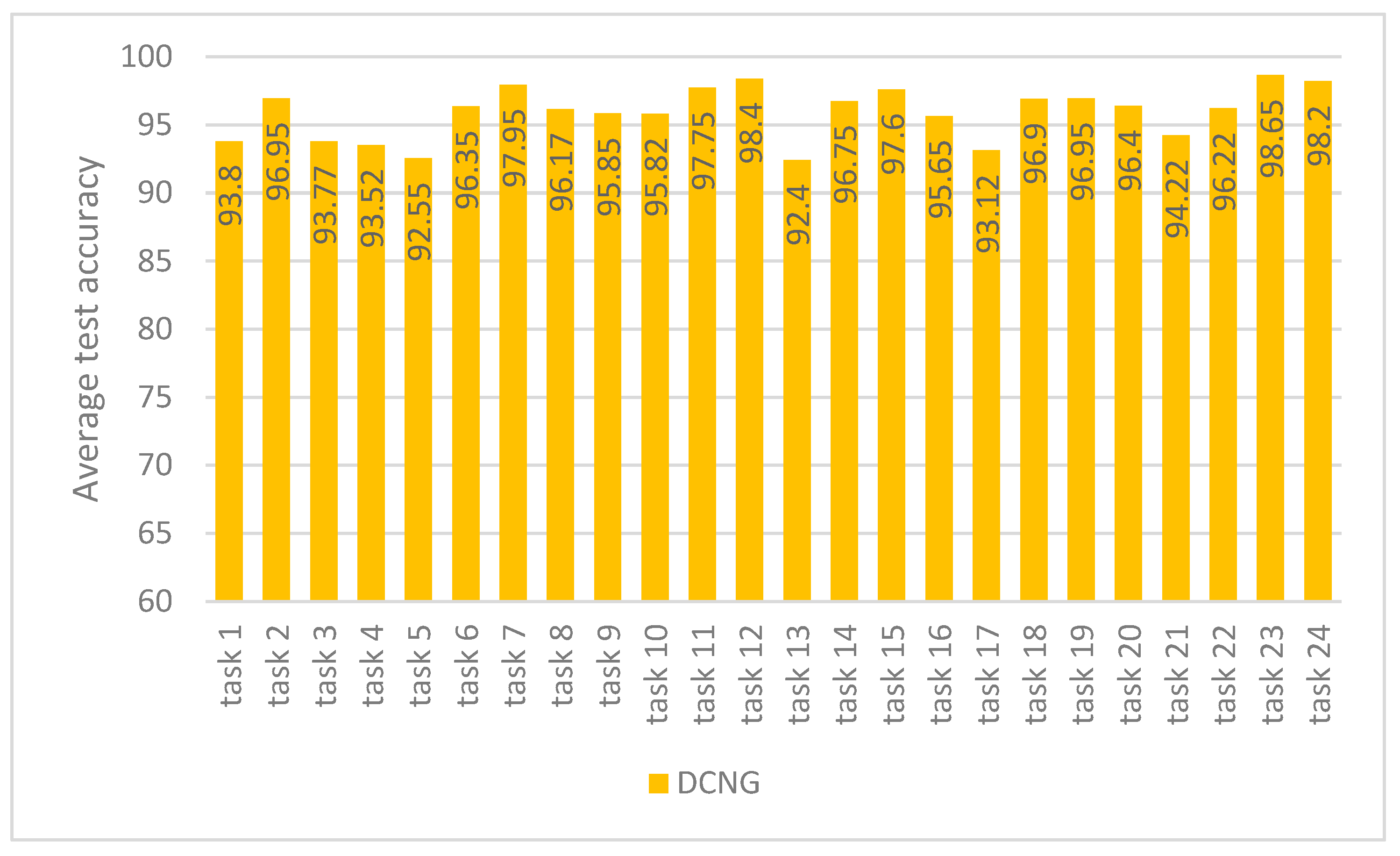
Figure 4 shows the results of DCNG on 24 transfer tasks in the CWRU dataset. It can be seen from the figure that the highest classification result is 98.65% on task 23 and the lowest classification result is 92.4% on task 13, with a 6.25% difference between them. NCNG performed above 92% on all transfer tasks.

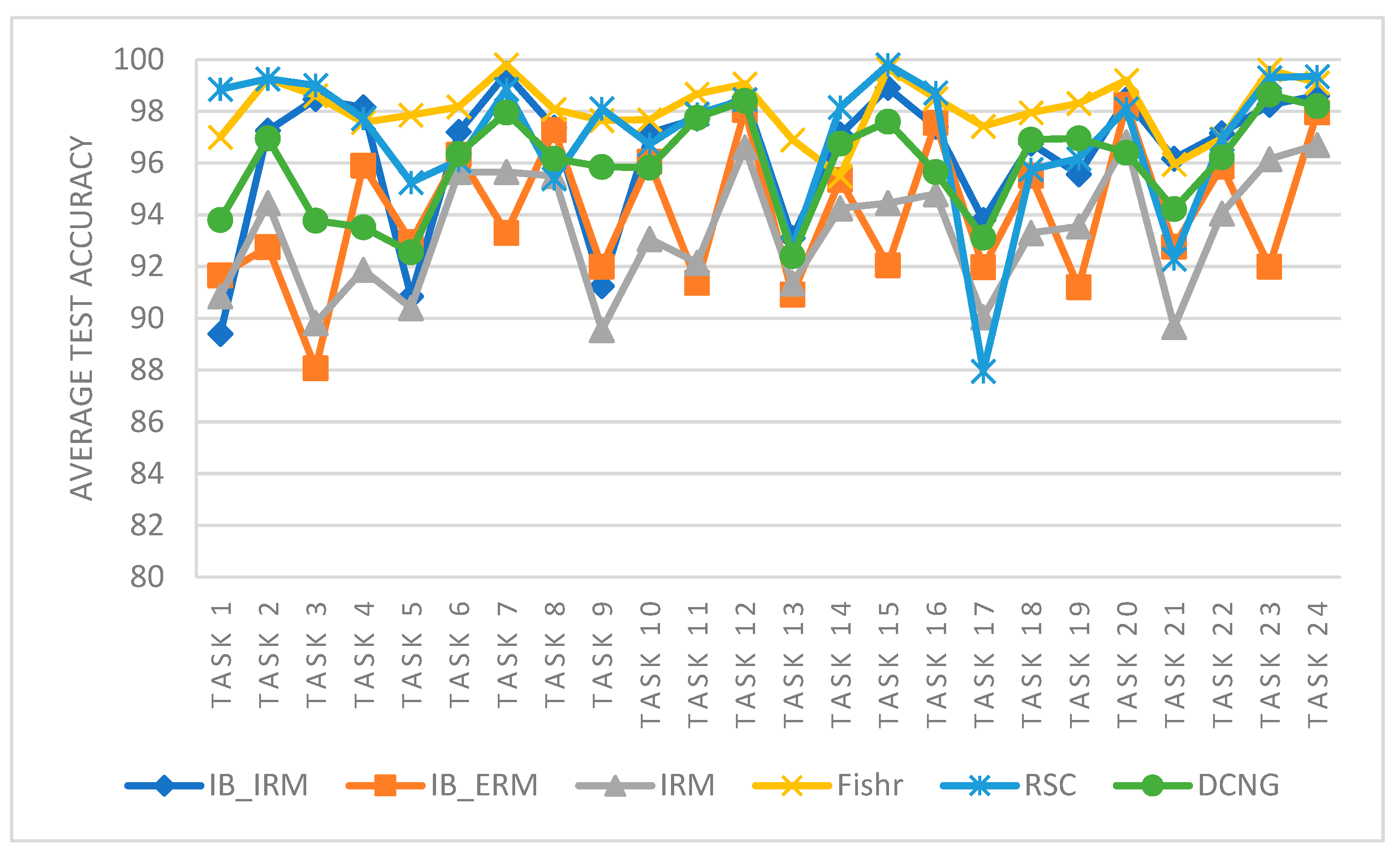
The performance of different generalization methods is analyzed from the perspective of a single task. As shown in Figure 5, the transfer performance of IB_IRM, IB_ERM, and IRM methods is lower than that of Fishr, RSC, and DCNG methods on a single task. For RSC and DCNG methods, the overall transfer result of RSC is higher than that of DCNG. However, in some transfer tasks, such as task 17, the performance of Fishr is lower than that of theDCNG method, and in the overall transfer tasks, the performance of Fishr is better than that of the DCNG model. The specific significance of the tasks is shown in

Table 2. DCNG transfer tasks on CWRU data sets.

Transfer Task	Source Domain	Target Domain
task 1	A, B	A
task 2	A, B	B
task 3	A, B	C
task 4	A, B	D
task 5	A, C	A
task 6	A, C	B
task 7	A, C	C
task 8	A, C	D
task 9	A, D	A
task 10	A, D	B
task 11	A, D	C
task 12	A, D	D
task 13	B, C	A
task 14	B, C	B
task 15	B, C	C
task 16	B, C	D
task 17	B, D	A
task 18	B, D	B
task 19	B, D	C
task 20	B, D	D
task 21	C, D	A
task 22	C, D	B
task 23	C, D	C
task 24	C, D	D

.

The performance of different generalization methods was analyzed from the perspective of the entire task. IB_IRM, IB_ERM, and IRM methods fluctuated greatly in each transfer task, especially in the odd transfer task. The Fishr method was the most stable and superior for the DCNG model. Although RSC performs better than the DCNG model on some transfer tasks, the results varied greatly between tasks and are not as stable as the DCNG model.

2.

Compared with other generalization methods on the MFPT data set

Compared with the CWRU data set, there were 90 transfer tasks on the MFPT data set, and the MFPT data set had larger variations in working conditions, which was conducive for exploring the influence of a single condition on the generalization method in the scenario of changing working conditions.

Table 3. Generalization performance of DCNG on MFPT dataset.

	Target	I	J	K	L	M	N
Source
I, J		100.00	100.00	100.00	99.75	100.00	97.25
I, K		100.00	100.00	100.00	99.37	100.00	94.00
I, L		100.00	100.00	100.00	100.00	100.00	100.00
I, M		100.00	100.00	100.00	100.00	100.00	99.00
I, N		100.00	100.00	100.00	100.00	100.00	100.00
J, K		100.00	100.00	100.00	100.00	100.00	100.00
J, L		100.00	100.00	100.00	100.00	100.00	100.00
J, M		100.00	100.00	100.00	100.00	100.00	100.00
J, N		100.00	100.00	100.00	100.00	100.00	100.00
K, L		100.00	100.00	100.00	100.00	100.00	100.00
K, M		100.00	100.00	100.00	100.00	100.00	100.00
K, N		99.87	100.00	100.00	100.00	100.00	100.00
L, M		100.00	100.00	100.00	100.00	100.00	100.00
L, N		100.00	100.00	100.00	100.00	100.00	100.00
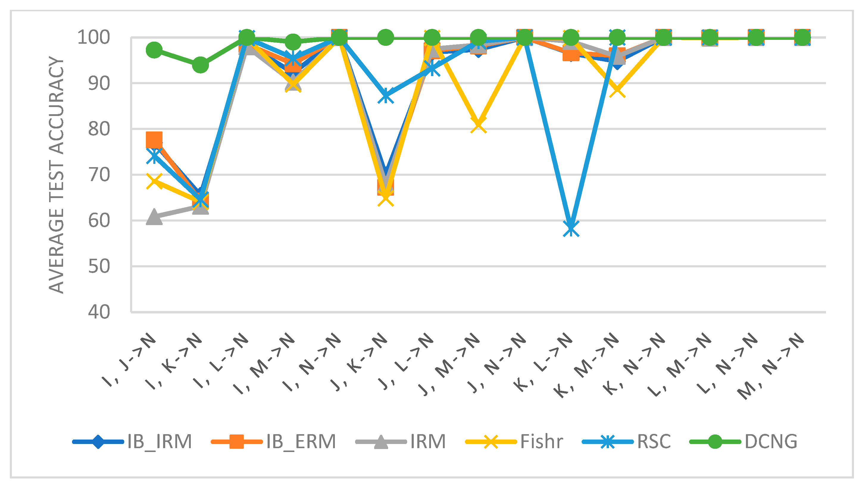
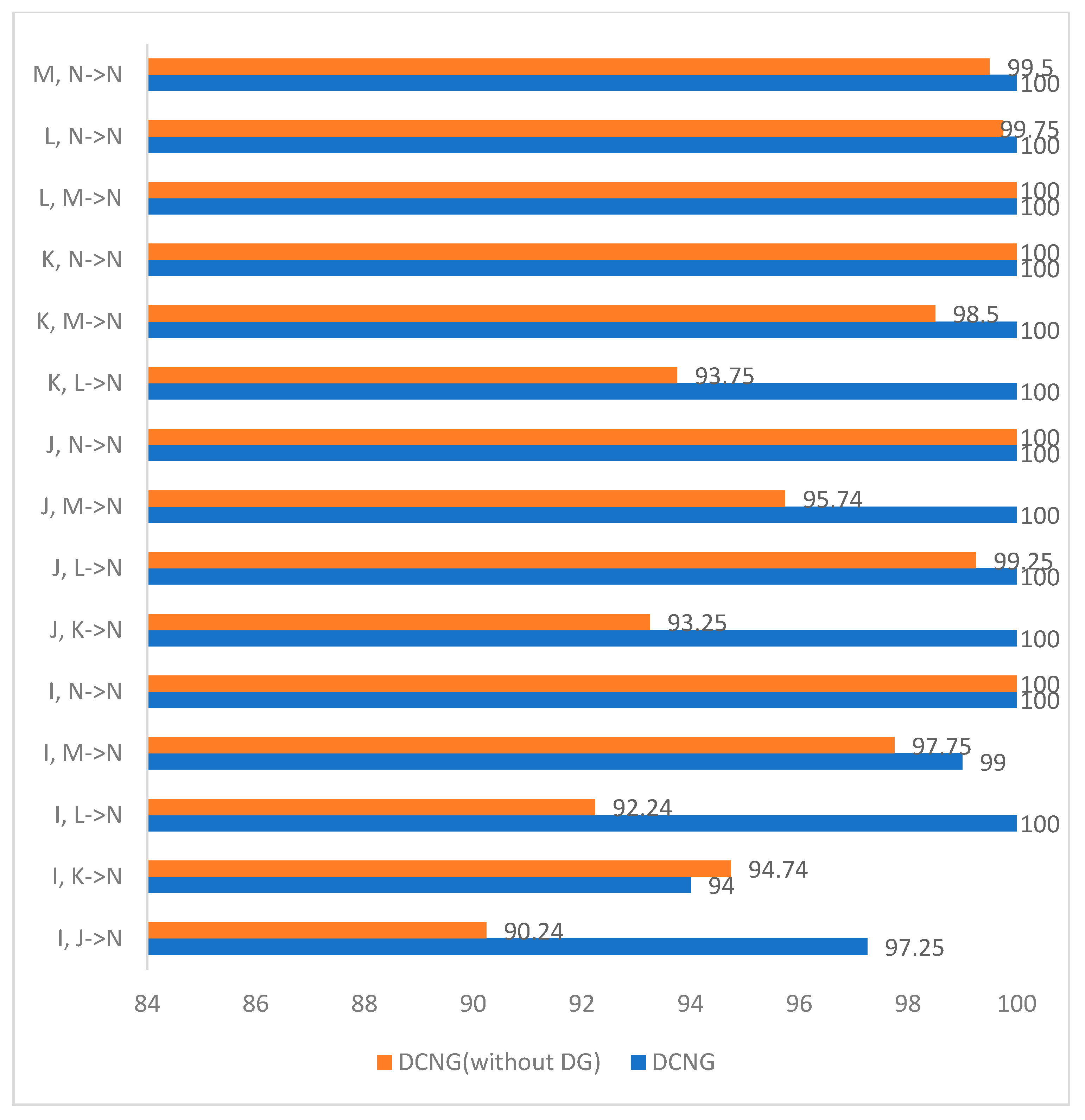
M, N		100.00	100.00	100.00	100.00	100.00	100.00

shows the results of DCNG model on 90 transfer tasks of MFPT data set. The average result of DCNG model on the transfer task of condition with target domain N is 99.35%, and the lowest result is 94% on the transfer task I, K-> N. Although the DCNG model achieved good results on different transfer tasks. However, when the “distance” of working conditions increased, transfer performance fluctuated.

As shown in Figure 6, the results of different generalization methods are almost the same for other tasks outside the target domain N; thus, only results of the condition transfer task with the target domain N are displayed. It can be seen from Figure 6 that the performance of IB_IRM, IB_ERM, IRM, and other methods is higher than that of I, J -> N, I, K -> N, and J, K -> N. In addition, these tasks all belong to tasks that do not contain condition N in the source domain and directly generalize condition N. The transfer results on these tasks indicate that IB_IRM, IB_ERM, and IRM methods have poor generalization performance in conditions with large “distance”.

For the DCNG model, although generalization performance fluctuates in the conditions with large “distance”, it has little impact on the transfer performance of the model on the overall task, so the DCNG model has better generalization performance compared with other generalization methods.

3.

Compared with other generalization methods on the KAT data set

In the KAT data set, there are four working conditions and a total of 24 transfer tasks. The performance of different generalization methods will be tested on 24 transfer tasks, as shown in

Table 4. DCNG transfer tasks on KAT data sets.

Transfer Task	Source Domain	Target Domain
task 1	E, F	E
task 2	E, F	F
task 3	E, F	G
task 4	E, F	H
task 5	E, G	E
task 6	E, G	F
task 7	E, G	G
task 8	E, G	H
task 9	E, H	E
task 10	E, H	F
task 11	E, H	G
task 12	E, H	H
task 13	F, G	E
task 14	F, G	F
task 15	F, G	G
task 16	F, G	H
task 17	F, H	E
task 18	F, H	F
task 19	F, H	G
task 20	F, H	H
task 21	G, H	E
task 22	G, H	F
task 23	G, H	G
task 24	G, H	H

.

Different from CWRU and MFPT datasets, KAT datasets have more operating conditions than the other two datasets, and the changes between working conditions are more complex and difficult to transfer. Transfer performance on KAT datasets can better reflect the size of model generalization abilities.

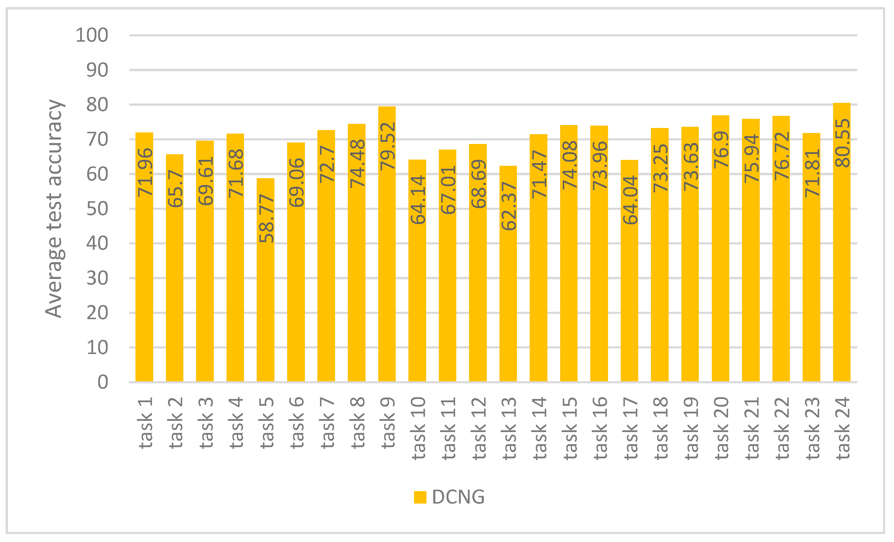
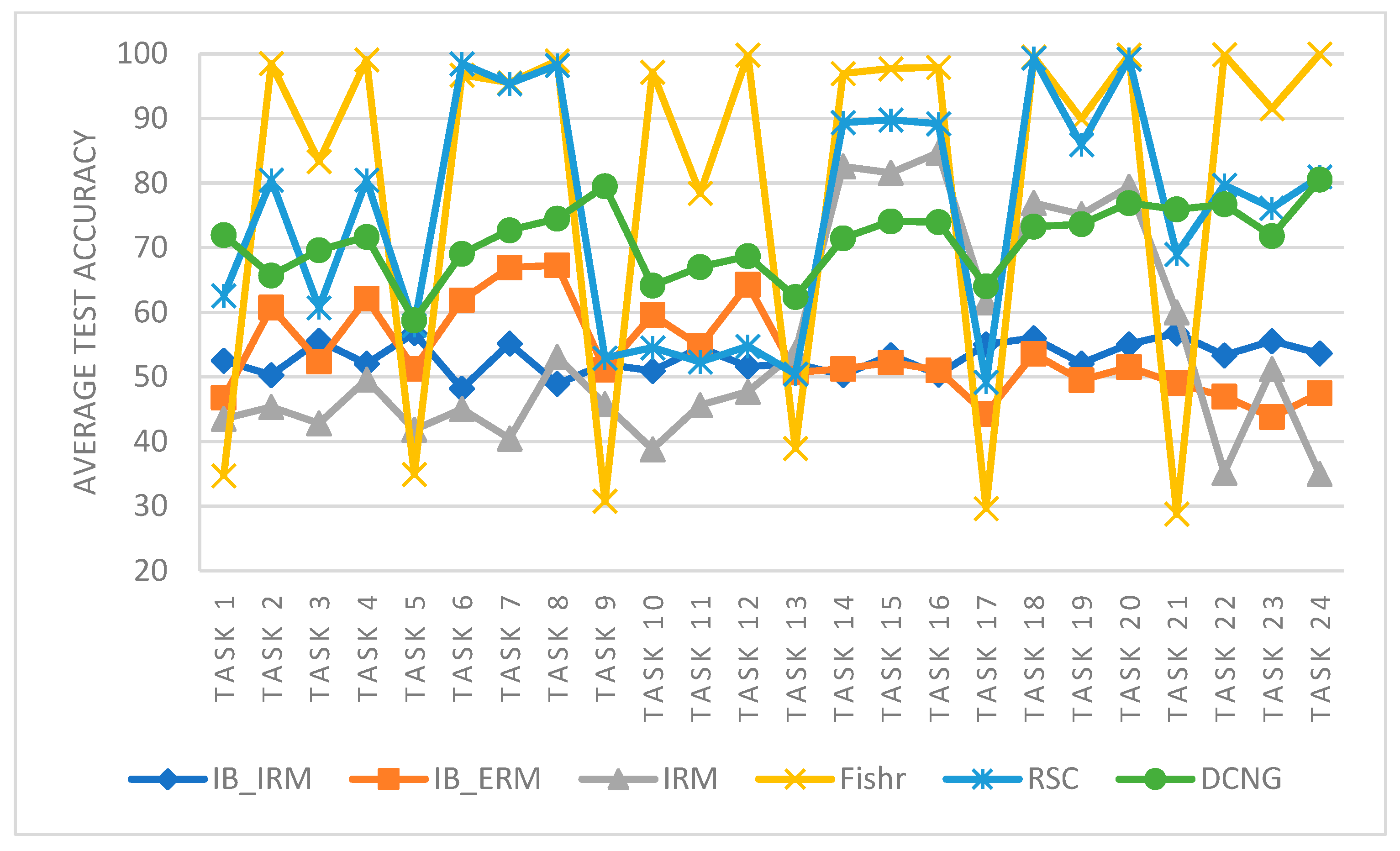
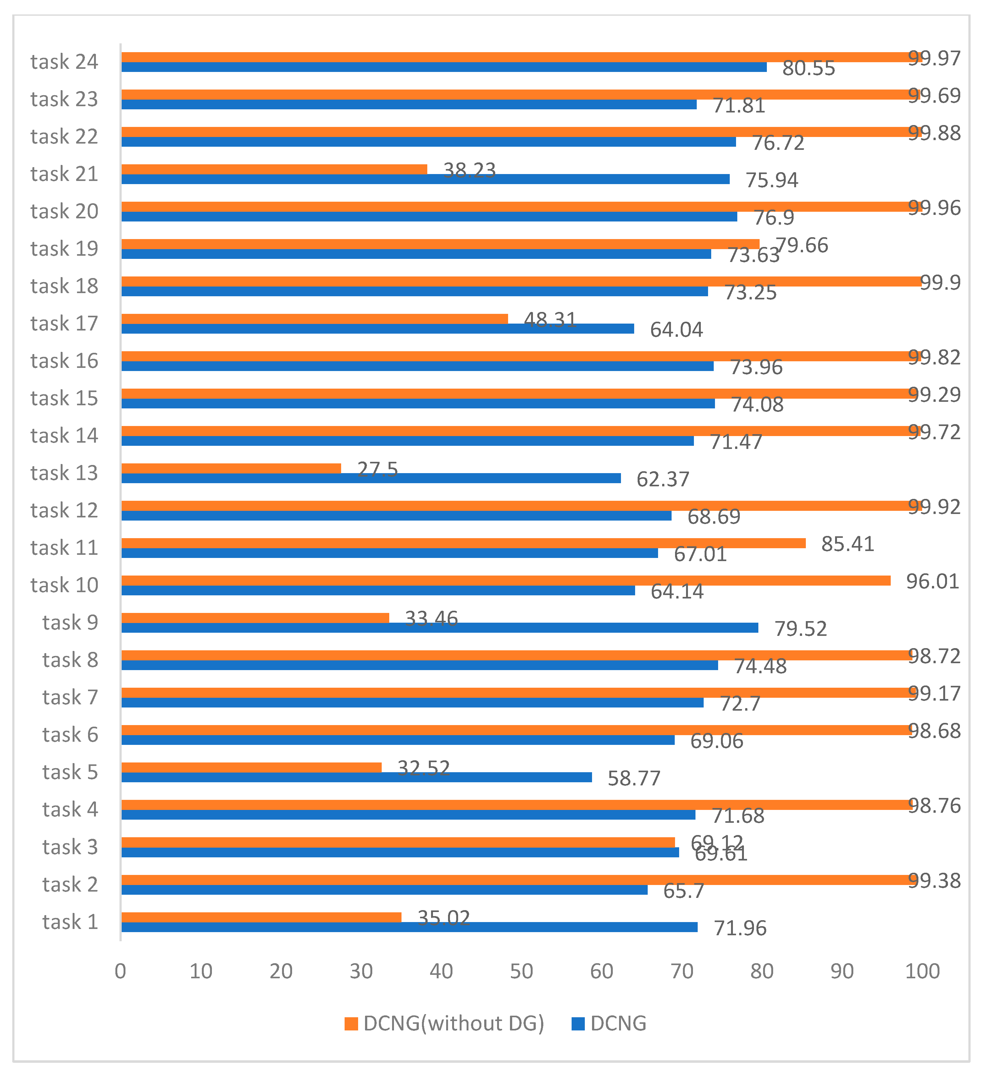
Figure 7 shows that the results of DCNG on 24 transfer tasks of the KAT data set. The highest transfer result is 80.55% on task 24 and the lowest transfer result is 58.77% on task 5, with a difference of 21.78%. The results on other tasks are all above 62%.

The average result of DCNG on the overall transfer task is 71.16%. When the “distance” of working conditions changes, it has little influence on the transfer performance of DCNG model, which is better than other generalization methods.

From the perspective of transfer performance of a single task, the variation range of Fishr, IRM, and RSC methods is larger than the other three methods, and the results of different transfer tasks are not stable, As shown in Figure 8. For IB_ERM and IB_IRM, the fluctuation range is small, but the overall transfer result is too low, and the result is about 50%. The DCNG method overcomes the instability of Fishr, IRM, and RSC methods, and it improves the transfer result of IB_ERM and IB_IRM methods, which has more application advantages in practical scenarios.

3.2.2. Influence of Different Parameter Settings on DCNG Model

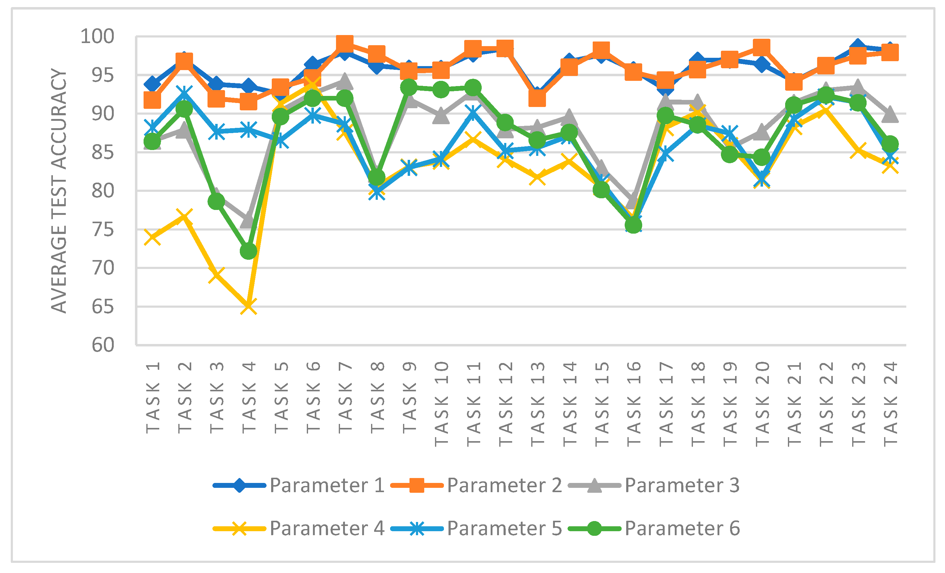
• Influence of different parameters on DCNG model in the CWRU data set

As shown in Figure 9, the performance of DCNG model in the CWRU data set under different parameter settings is shown in

Table 5. Different parameter settings on the CWRU data set.

Parameter Settings	τ	ρ
Parameter 1	0.4	100.0
Parameter 2	0.45	100.0
Parameter 3	0.5	100.0
Parameter 4	0.5	1000.0
Parameter 5	0.6	100.0
Parameter 6	0.65	100.0

. From the perspective of different tasks, even in the same task, different parameter settings will affect the transfer performance of DCNG model. When $\tau$ values of parameters 1, 2, 5, and 6 increase and $\rho$ values remain constant, the DCNG model’s effect on the transfer task decreases and the larger $\tau$ value increases, which is more obvious on task 1 and task 4. The value of $\rho$ increases and the value of $\tau$ remains constant in the settings of parameter 3 and parameter 4 and the performance of transfer decreases gradually, which is more obvious in the first 15 transfer tasks.

From the observation of the entire transfer task, it can be analyzed that with an increase in $\rho$ and $\tau$ values, the transfer results of DCNG model in the entire CWRU data set fluctuated more and more, and the stability of the model became worse. The optimal model parameters are $\rho =100.0 \mathrm{and} \tau =0.4$.

2.

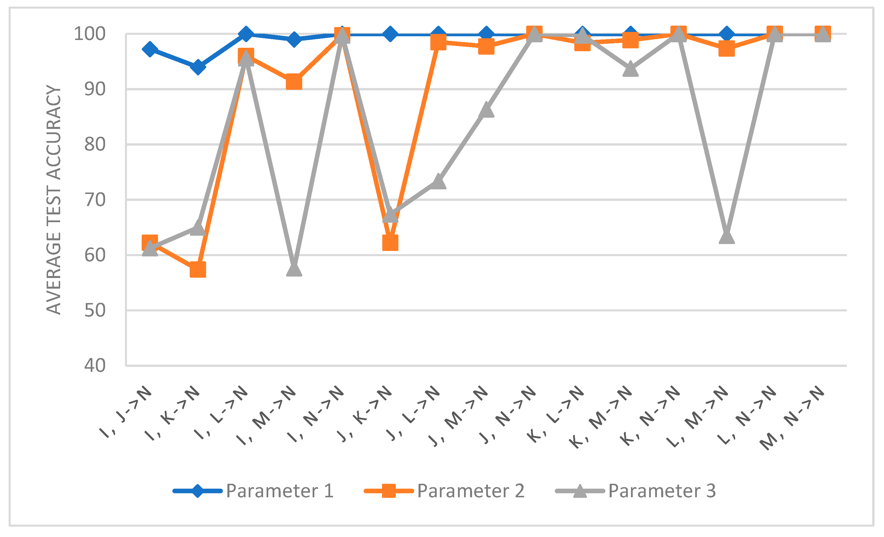
Influence of different parameters on the DCNG model in the MFPT data set

Figure 10 shows the performance of DCNG model under different parameter settings on the MFPT dataset. Since both CWRU and MFPT datasets belong to the scenario where the working condition changes due to a single condition, the influence of parameter ρ is not as great as that of the τ value. Therefore, for the ρ value, we selected the optimal value in the CWRU data set and the specific parameter settings are shown in

Table 6. Different parameter settings on the MFPT data set.

Parameter Settings	τ	ρ
Parameter 1	0.4	100.0
Parameter 2	0.5	100.0
Parameter 3	0.6	100.0

. With the increase in τ, the transfer performance on a single transfer task begins to decrease. From I, J -> N and I, K -> N, the transfer results of N and other tasks can still be analyzed, and it can be concluded that the difficulty of transfers will increase with the increase in the “distance” of working conditions and the performance of the transfer task with the large “distance” of working conditions is an important basis to investigate the model’s generalization ability.

It can be observed from the entire transfer task that the DCNG model “wobbles” in the transfer task with the increase in τ value, and the generalization ability of DCNG model decreases. The optimal parameters are ρ = 100.0 and τ = 0.4.

3.

Influence of different parameters on DCNG model in KAT data set

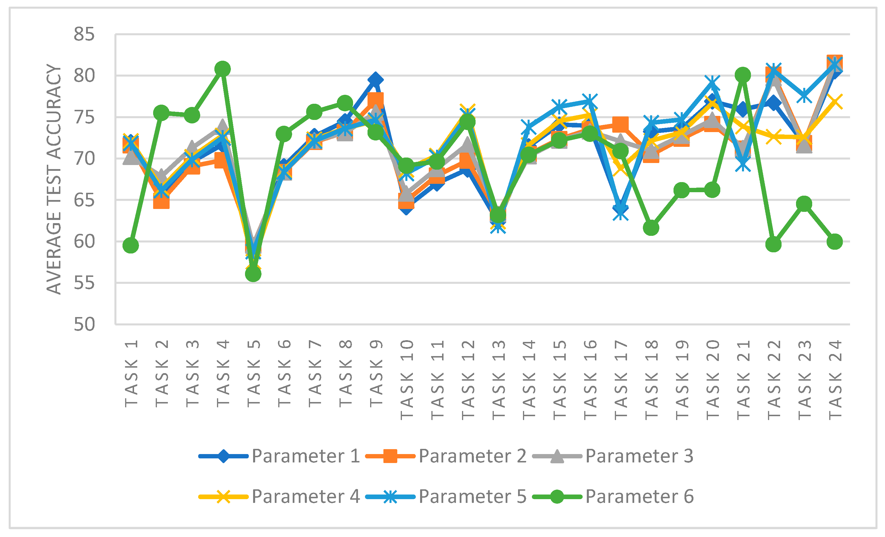
Figure 11 shows the performance of the DCNG model under different parameter settings on the KAT data set, As shown in

Table 7. Different parameter settings on KAT data set.

Parameter Settings	τ	ρ
Parameter 1	0.6	100.0
Parameter 2	0.6	500.0
Parameter 3	0.6	1000.0
Parameter 4	0.65	100.0
Parameter 5	0.7	100.0
Parameter 6	0.8	100.0

. It can be directly observed from the figure that the transfer performance of DCNG model in KAT transfer task is lower than that of the CWRU data set and MFPT data set, and the degree of “jitter” is more severe than that of the two data sets. The results show that the scenarios with multiple conditions leading to the change of working conditions are more complex and more difficult to transfer than those with single conditions. τ values of parameters 1, 4, 5, and 6 increase while ρ values remain constant, and the performance of the model decreases in different degrees for each transfer task. The values of ρ in parameters 1, 2, and 3 increase continuously, while τ remains constant. The performance of the DCNG model on transfer task does not change significantly.

Observed from the entire transfer task, the results of DCNG model varied roughly between 55 and 80%. There was a large performance gap between different transfer tasks, indicating that the change of “distance” between working conditions was more complex and challenging for the generalization ability of the model in the scenario where multiple conditions led to a change in working conditions. The optimal parameters of DCNG model on KAT data set are ρ = 100.0 and τ = 0.6.

3.2.3. Compared with the Model without SAND Mask

• Compare the generalized model DCNG and the ungeneralized model on the CWRU data set

Figure 12 shows the comparison between the generalized model DCNG and the ungeneralized model on the CWRU data set, where the ungeneralized model represents the same network structure as the model DCNG but without generalization measure SAND-Mask. The average transfer result of the ungeneralized model on the entire transfer task is 97.43%, the highest transfer result on task 7 is 99.69%, and the lowest transfer result on task 10 is 93.04%. The average transfer result of the generalized model DCNG on the overall transfer task was 95.91%, the highest transfer result on task 23 was 98.65%, and the lowest transfer result on task 13 was 92.4%.

The average transfer performance of the ungeneralized model is 1.52% higher than that of the DCNG model, indicating that the smaller “distance” between the working conditions is easier to generalize in the scenario where the single condition causes a change in working conditions and the DCNG model has a good generalization effect on the CWRU data set.

2.

Compare the generalized model DCNG and the ungeneralized model on the MFPT data set

The DCNG model without generalization measures was compared with the generalized model, and the results of the DCNG model without generalization measures on the MFPT dataset are shown in

Table 8. Performance of ungeneralized model DCNG on MFPT dataset.

	Target	I	J	K	L	M	N
Source
I, J		100.00	100.00	100.00	100.00	100.00	90.24
I, K		100.00	100.00	100.00	99.75	100.00	94.74
I, L		100.00	100.00	100.00	100.00	100.00	92.24
I, M		100.00	100.00	100.00	99.75	100.00	97.75
I, N		100.00	100.00	100.00	100.00	100.00	100.00
J, K		100.00	100.00	100.00	99.75	100.00	93.25
J, L		99.50	100.00	100.00	100.00	100.00	99.25
J, M		88.24	97.24	97.24	100.00	100.00	95.74
J, N		100.00	100.00	100.00	99.75	100.00	100.00
K, L		100.00	100.00	100.00	100.00	100.00	93.75
K, M		100.00	100.00	100.00	100.00	100.00	98.50
K, N		99.50	100.00	100.00	100.00	100.00	100.00
L, M		98.50	100.00	99.75	100.00	100.00	100.00
L, N		97.49	99.75	99.75	100.00	100.00	99.75
M, N		100.00	100.00	100.00	100.00	100.00	99.50

.

Figure 13 shows the comparison between the results of the generalized model DCNG and the ungeneralized model on 15 transfer tasks with N working conditions as the target domain in the MFPT dataset. The results of the ungeneralized model on the transfer task with N working conditions as the target domain are quite different from those of the DCNG model, so we only compare the results on the migration task with N working conditions as the target domain. The average result of the ungeneralized model on 15 transfer tasks is 96.98%, while the average result of the generalized model on 15 transfer tasks is 99.35%.

There is a 2.37% difference between the average transfer results of the generalized model and the ungeneralized model. Relatively speaking, the performance of the ungeneralized model fluctuates greatly in the transfer task with N conditions as the target domain, and the model is greatly affected by the “distance” of conditions.

The stability of the model on MFPT data set is lower than that on the CWRU data set, indicating that the “distance” of operating conditions increases when operating conditions change, and the direct generalization of operating conditions in the target domain cannot meet actual requirements.

3.

Compare the generalized model DCNG and the ungeneralized model on the KAT data set

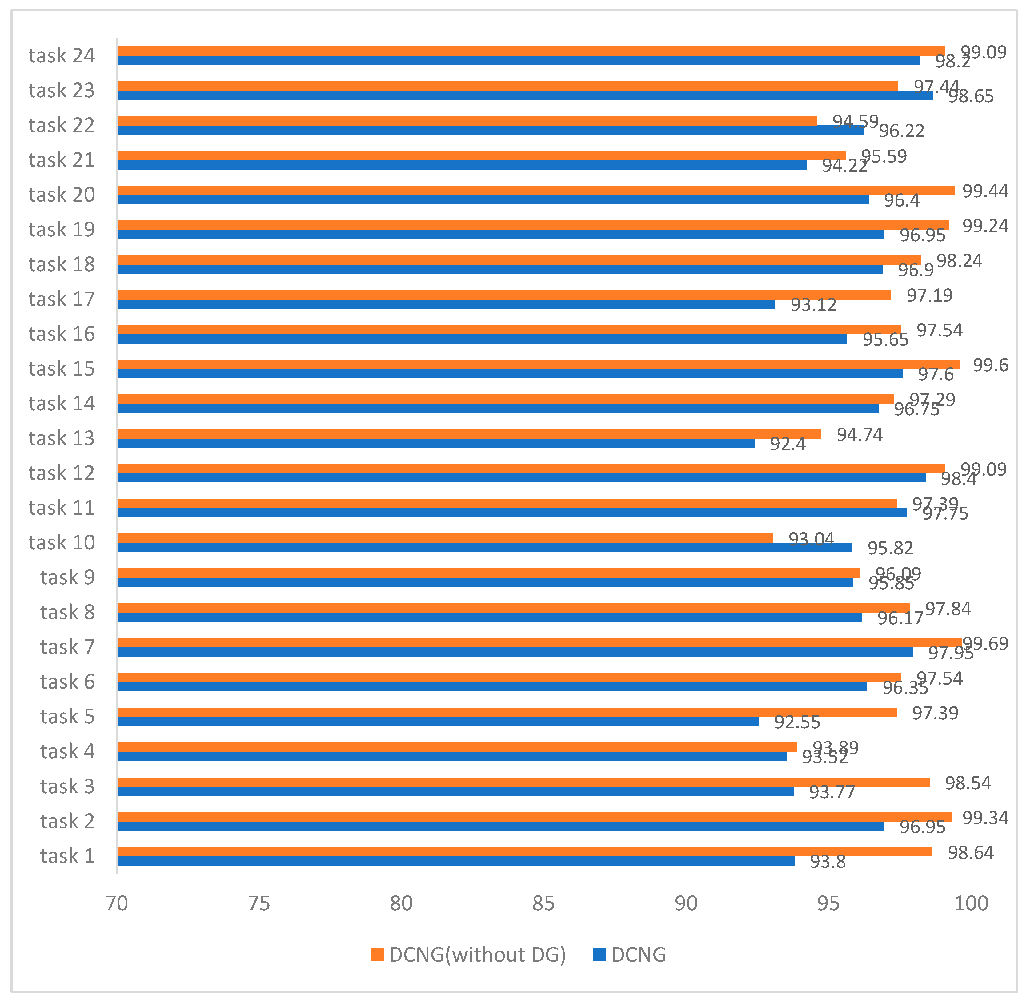
Figure 14 shows the comparison between the results of the generalized model DCNG and the ungeneralized model in 24 transfer tasks of KAT data set. The average result of the ungeneralized model on the overall transfer task was 80.75%, among which the transfer result on task 24 was 99.97%, and the transfer result on task 13 was 27.5%, with a difference of 72.47%. The average transfer result of the generalized model DCNG on the overall transfer task was 71.16%, the highest transfer result on task 24 was 80.55%, and the lowest transfer result on task 5 was 58.77%, with a 21.78% difference between them. Although the effect of the ungeneralized model on some transfer tasks is higher than that of the generalized model DCNG, the effect of the ungeneralized model on different transfer tasks is not balanced, and the maximum gap can reach 72.47%. In a sense, the ungeneralized model is invalid in some transfer tasks.

According to the performance of the generalization model on each transfer task in Figure 14, it can be found that the transfer effect on task 1, task 3, task 5, task 9, task 13, task 17, and task 21 is worse than other tasks. From Table 4, we found that the task’s working condition of the target domain of migration is E; from a physical sense, E’s speed change is larger than that of the other conditions and the ungeneralized model is almost ineffectual for these tasks. Although the transfer effect of the generalized model DCNG on the KAT data set does not reach more than 80%, the DCNG model has good stability and is less affected by the change of working conditions; thus, it has a very promising prospect for engineering applications in practical scenarios.

4. Discussion

Based on the experimental comparison between DCNG model and different generalization methods, the influence of different parameters on DCNG model, and the experimental comparison between the generalized model DCNG and the ungeneralized model, we can conclude that the DCNG model is more stable and better than other methods, and it is less affected by the variation of working conditions, and it has better generalization performance. In addition, the increase in the “distance” of working conditions in both scenarios will have an impact on the generalization performance of the model for scenarios where single conditions cause working conditions to change and scenarios where multiple conditions cause working conditions to change. However, in the scenario where multiple conditions lead to changes in operating conditions, the influences of different operating conditions on diagnosis results and of “distance” between operating conditions on diagnosis results are not clear. We will conduct further research on this in the future.

5. Conclusions

In this paper, the problem of domain shift in fault diagnosis and previous work on domain shift solutions are described, and a similarity in the variance between the data of different working conditions was found. The DCNG model and the generalization method SAND-Mask used are proposed. Combined with the characteristics of fault diagnosis domain data, the method of calculating gradient variance of SAND-Mask method was improved, and the domain generalization method was used to solve the fault diagnosis problem in scenarios where working condition data could not be obtained. Relevant experiments were carried out on CWRU data sets, MFPT data sets, and KAT data sets with different characteristics. The validity of the proposed generalization model DCNG is proved.

References

1. Guo, L.; Li, N.; Jia, F.; Lei, Y.; Lin, J. A recurrent neural network based health indicator for remaining useful life prediction of bearings. Neurocomputing 2017, 240, 98–109. [Google Scholar] [CrossRef]
2. Pan, H.; He, X.; Tang, S.; Meng, F. An Improved Bearing Fault Diagnosis Method using One-Dimensional CNN and LSTM. Stroj. Vestn. J. Mech. Eng. 2018, 64, 443–452. [Google Scholar]
3. Jiang, H.; Li, X.; Shao, H.; Zhao, K. Intelligent fault diagnosis of rolling bearings using an improved deep recurrent neural network. Meas. Sci. Technol. 2018, 29, 065107. [Google Scholar] [CrossRef]
4. Zhang, W.; Li, X.; Ding, Q. Deep residual learning-based fault diagnosis method for rotating machinery. ISA Trans. 2019, 95, 295–305. [Google Scholar] [CrossRef]
5. Zhao, M.; Kang, M.; Tang, B.; Pecht, M. Deep residual networks with dynamically weighted wavelet coefficients for fault diagnosis of planetary gearboxes. IEEE Trans. Ind. Electron. 2017, 65, 4290–4300. [Google Scholar] [CrossRef]
6. Li, X.; Zhang, W.; Ma, H.; Zhong, L.; Xu, L. Domain generalization in rotating machinery fault diagnostics using deep neural networks. Neurocomputing 2020, 403, 409–420. [Google Scholar] [CrossRef]
7. Liao, Y.; Huang, R.; Li, J.; Chen, Z.; Li, W. Deep semisupervised domain generalization network for rotary machinery fault diagnosis under variable speed. IEEE Trans. Instrum. Meas. 2020, 69, 8064–8075. [Google Scholar]
8. Shahtalebi, S.; Gagnon-Audet, J.C.; Laleh, T.; Faramarzi, M.; Ahuja, K.; Rish, I. Sand-mask: An enhanced gradient masking strategy for the discovery of invariances in domain generalization. arXiv 2021, arXiv:2106.02266. [Google Scholar]
9. Yang, B.; Lei, Y.; Jia, F.; Xing, S. An intelligent fault diagnosis approach based on transfer learning from laboratory bearings to locomotive bearings. Mech. Syst. Signal Process. 2019, 122, 692–706. [Google Scholar] [CrossRef]
10. Chen, C.; Li, Z.; Yang, J.; Liang, B. A cross domain feature extraction method based on transfer component analysis for rolling bearing fault diagnosis. In Proceedings of the 2017 29th Chinese Control and Decision Conference (CCDC), Chongqing, China, 28–30 May 2017; pp. 5622–5626. [Google Scholar]
11. Xie, J.; Zhang, L.; Duan, L.; Wang, J. On cross-domain feature fusion in gearbox fault diagnosis under various operating conditions based on transfer component analysis. In Proceedings of the 2016 IEEE International Conference on Prognostics and Health Management (ICPHM), Ottawa, ON, Canada, 20–22 June 2016; pp. 1–6. [Google Scholar]
12. Tong, Z.; Li, W.; Zhang, B.; Jiang, F.; Zhou, G. Bearing fault diagnosis under variable working conditions based on domain adaptation using feature transfer learning. IEEE Access 2018, 6, 76187–76197. [Google Scholar] [CrossRef]
13. Tong, Z.; Li, W.; Zhang, B.; Zhang, M. Bearing fault diagnosis based on domain adaptation using transferable features under different working conditions. Shock. Vib. 2018, 2018 Pt 6, 6714520.1–6714520.12. [Google Scholar] [CrossRef]
14. Gretton, A.; Borgwardt, K.M.; Rasch, M.J.; Schölkopf, B.; Smola, A. A kernel two-sample test. J. Mach. Learn. Res. 2012, 13, 723–773. [Google Scholar]
15. Zhang, W.; Li, C.; Peng, G.; Chen, Y.; Zhang, Z. A deep convolutional neural network with new training methods for bearing fault diagnosis under noisy environment and different working load. Mech. Syst. Signal Process. 2018, 100, 439–453. [Google Scholar] [CrossRef]
16. Lu, W.; Liang, B.; Cheng, Y.; Meng, D.; Yang, J.; Zhang, T. Deep model based domain adaptation for fault diagnosis. IEEE Trans. Ind. Electron. 2016, 64, 2296–2305. [Google Scholar] [CrossRef]
17. Wen, L.; Gao, L.; Li, X. A new deep transfer learning based on sparse auto-encoder for fault diagnosis. IEEE Trans. Syst. Man Cybern. Syst. 2017, 49, 136–144. [Google Scholar] [CrossRef]
18. Zheng, H.; Wang, R.; Yang, Y.; Li, Y.; Xu, M. Intelligent fault identification based on multisource domain generalization towards actual diagnosis scenario. IEEE Trans. Ind. Electron. 2019, 67, 1293–1304. [Google Scholar] [CrossRef]
19. Zhang, R.; Tao, H.; Wu, L.; Guan, Y. Transfer learning with neural networks for bearing fault diagnosis in changing working conditions. IEEE Access 2017, 5, 14347–14357. [Google Scholar] [CrossRef]
20. Hasan, M.J.; Kim, J.M. Bearing fault diagnosis under variable rotational speeds using stockwell transform-based vibration imaging and transfer learning. Appl. Sci. 2018, 8, 2357. [Google Scholar] [CrossRef] [Green Version]
21. Han, T.; Liu, C.; Yang, W.; Jiang, D. Deep transfer network with joint distribution adaptation: A new intelligent fault diagnosis framework for industry application. ISA Trans. 2020, 97, 269–281. [Google Scholar] [CrossRef] [Green Version]
22. Xu, Y.; Sun, Y.; Liu, X.; Zheng, Y. A digital-twin-assisted fault diagnosis using deep transfer learning. IEEE Access 2019, 7, 19990–19999. [Google Scholar] [CrossRef]
23. Shao, S.; McAleer, S.; Yan, R.; Baldi, P. Highly accurate machine fault diagnosis using deep transfer learning. IEEE Trans. Ind. Inform. 2018, 15, 2446–2455. [Google Scholar] [CrossRef]
24. Li, X.; Zhang, W.; Ding, Q.; Li, X. Diagnosing rotating machines with weakly supervised data using deep transfer learning. IEEE Trans. Ind. Inform. 2019, 16, 1688–1697. [Google Scholar] [CrossRef]
25. Zheng, H.; Yang, Y.; Yin, J.; Li, Y.; Wang, R.; Xu, M. Deep domain generalization combining a priori diagnosis knowledge toward cross-domain fault diagnosis of rolling bearing. IEEE Trans. Instrum. Meas. 2020, 70, 1–11. [Google Scholar] [CrossRef]
26. Wang, J.; Lan, C.; Liu, C.; Ouyang, Y.; Qin, T.; Lu, W.; Chen, Y.; Zeng, W.; Yu, P. Generalizing to unseen domains: A survey on domain generalization. arXiv 2021, arXiv:2103.03097. [Google Scholar]
27. Parascandolo, G.; Neitz, A.; Orvieto, A.; Gresele, L.; Schölkopf, B. Learning explanations that are hard to vary. arXiv 2020, arXiv:2009.00329. [Google Scholar]
28. Ragab, M.; Chen, Z.; Wu, M.; Li, H.; Kwoh, C.K.; Yan, R.; Li, X. Adversarial multiple-target domain adaptation for fault classification. IEEE Trans. Instrum. Meas. 2020, 70, 1–11. [Google Scholar] [CrossRef]
29. The Case Western Reserve University Bearing Data Center Website. Bearing Data Center Test Seeded Fault Test Data. Available online: http://csegroups.case.edu/bearingdatacenter/pages/download-data-file (accessed on 1 February 2021).
30. Society for Machinery Failure Prevention Technology. MFPT Dataset. Available online: https://mfpt.org/fault-datasets/ (accessed on 12 February 2021).
31. Paderborn University. Bearing Data Center. Available online: https://mb.uni-paderborn.de/kat/forschung/datacenter/bearing-datacenter/ (accessed on 1 February 2021).
32. Ahuja, K.; Caballero, E.; Zhang, D.; Gagnon-Audet, J.C.; Bengio, Y.; Mitliagkas, I.; Rish, I. Invariance principle meets information bottleneck for out-of-distribution generalization. Adv. Neural Inf. Processing Syst. 2021, 34, 3438–3450. [Google Scholar]
33. Arjovsky, M.; Bottou, L.; Gulrajani, I.; Lopez-Paz, D. Invariant risk minimization. arXiv 2019, arXiv:1907.02893. [Google Scholar]
34. Rame, A.; Dancette, C.; Cord, M. Fishr: Invariant gradient variances for out-of-distribution generalization. arXiv 2021, arXiv:2109.02934. [Google Scholar]
35. Huang, Z.; Wang, H.; Xing, E.P.; Huang, D. Self-challenging improves cross-domain generalization. In Proceedings of the European Conference on Computer Vision, Cham, Switzerland, 23 August 2020; pp. 124–140. [Google Scholar]
Figure 1. DCNG network.
Algorithms 15 00215 g001
Figure 2. SAND-Mask Calculates σ in a batch.
Algorithms 15 00215 g002
Figure 3. The gradient variance of all samples in the batch replaces the gradient variance of each sample.
Algorithms 15 00215 g003
Figure 4. Generalization performance of DCNG on CWRU data sets.
Algorithms 15 00215 g004
Figure 5. Performance comparison of different generalization methods on CWRU data sets.
Algorithms 15 00215 g005
Figure 6. Performance comparison of different generalization methods on MFPT data sets.
Algorithms 15 00215 g006
Figure 7. Generalization performance of DCNG on KAT data sets.
Algorithms 15 00215 g007
Figure 8. Performance comparison of different generalization methods on KAT data sets.
Algorithms 15 00215 g008
Figure 9. The influence of different parameter settings on the DCNG model in the CWRU data set.
Algorithms 15 00215 g009
Figure 10. The influence of different parameter Settings on DCNG model in MFPT data set.
Algorithms 15 00215 g010
Figure 11. The influence of different parameter settings on DCNG model in KAT data set.
Algorithms 15 00215 g011
Figure 12. DCNG and ungeneralized model performance on 24 tasks in the CWRU dataset.
Algorithms 15 00215 g012
Figure 13. DCNG and ungeneralized model performance on 15 tasks in the MFPT dataset.
Algorithms 15 00215 g013
Figure 14. DCNG and ungeneralized model performance on 24 tasks in the KAT dataset.
Algorithms 15 00215 g014