Article

Study of Motion Control and a Virtual Reality System for Autonomous Underwater Vehicles

Faculty of Computer, Guangdong University of Technology, Guangzhou 510006, China
*
Author to whom correspondence should be addressed.
Algorithms 2021, 14(3), 93; https://doi.org/10.3390/a14030093
Submission received: 10 February 2021 / Revised: 14 March 2021 / Accepted: 14 March 2021 / Published: 18 March 2021

Abstract

:
This paper studies a novel intelligent motion control algorithm for Autonomous Underwater Vehicles (AUV) and develops a virtual reality system for a new interactive experimental platform. The paper designs a robust neuro-fuzzy controller to tackle system uncertainties and external disturbances. Fuzzy control can solve the uncertainty problem of control systems. The neural network model self-tunes the controller parameters to improve the anti-interference ability. The designed control algorithm is verified using a MATLAB implementation and a virtual reality system. The virtual reality system developed in this paper can be used to debug the control algorithm, simulate the marine environment, and establish an ocean current interference model. The paper uses the MATLAB engine to realize the data communication between the MATLAB and the AUV virtual reality system. This allows the output order of the controller in MATLAB to drive the AUV in a virtual simulation system to simulate the 3D space motion.

1. Introduction

AUV is a tightly coupled system which has to cope with high nonlinearity, uncertain motion, and severe disturbances. These requirements of the system lead to great challenges for motion control in AUVs. AUVs are used to perform a variety of tasks such as the detection of submarine oil pipeline and cables, the exploration of landform and landscape, the marine observation and analysis of sea level, as well as military application. In all these tasks, an AUV must track specific curves efficiently and accurately. Therefore, motion control is an important technology requirement for AUV research. Presently, researchers worldwide are actively developing AUV control algorithms. Frequently-used AUV control methods are: PID control, sliding mode control, adaptive control, back-stepping method, neural network control, and fuzzy control, and among others. For AUV navigation in a complex marine environment, interference factors such as ocean currents and sea waves vary at different working sea areas and depths. Apart from the maneuverability of the robotic motion, AUV navigation needs to also consider factors such as anti-swinging, stability, and sea-keeping analysis. However, in the complex environment of an ocean, directly using an AUV for experiments not only has high economic costs, but also presents a high risk. Various uncertain factors may easily result in the exposure of experimental devices to perilous environments. This can affect the security of the device and even lead to possible damages to the AUV during experiments. To tackle these challenges, the virtual AUV motion control platform has become a key topic in AUV research.
The path and trajectory tracking control of AUV are generally divided into two levels: kinematics and dynamics. Based on the line of sight method (LOS) and vector field method (VF) guiding law, a path tracking controller for underactuated vehicle is designed in literature [1,2]. A nonlinear backstepping technique based on virtual control variables is employed to design the kinematics and dynamics controllers for the three-dimensional trajectory tracking control of an underactuated autonomous underwater vehicle with unknown current disturbances [3]. However, when there are disturbances such as ocean current, path tracking based on traditional LOS and VF guiding laws will produce steady-state errors. In order to solve this problem, a guiding law of integrated line of sight method (ILOS) was proposed in the literature [4], which has been widely used. There has also been a lot of research on the design of path-following dynamic controllers for underactuated AUVs. Literature [5] applied the ILOS guidance law and PID controller to realize the horizontal path tracking control of underactuated AUV under ocean current disturbance. Literature [6] designed an adaptive controller and a sliding mode controller for the horizontal plane and vertical plane path tracking, respectively. The above literatures only consider the path tracking problem of AUV in the horizontal plane or vertical plane. Literature [7] applied linear stability theory and backstepping method to design a three-dimensional trajectory tracking controller for underactuated AUV. However, the influence of ocean current is not considered in the above 3D path tracking controllers.
Since AUV itself has characteristics of uncertainty and non-linearity, coupled with the interference of ocean current, it becomes very difficult to design such a controller. The purpose of path tracking is to reduce the state error of a robot. There are several problems that must be solved; among them, the most difficult and challenging are the highly nonlinear dynamics of the AUV and the uncertainty of the underwater dynamic parameters. The traditional control hardly avoids the problems, such as difficult adjustment of controller parameters, and the robustness.
To address the above problems, the intelligent control technologies such as fuzzy control, neural network have been gradually used in AUV tracking control, since the intelligent control technology requires no mathematical model and the system has good robustness. Fuzzy control is an effective approach to resolve the control problem of the uncertainty system. The neural network is very strong in self-learning.
A kind of neuro-fuzzy controller for AUV tracking proposed in this paper is a fuzzy system based on a neural network, which applies the learning function of a neural network to a fuzzy system so that the fuzzy system can automatically adjust and obtain fuzzy rules and membership parameters from the learning. The neuro-fuzzy model can constantly modify the membership function of the fuzzy subset and update it automatically, so it is a fuzzy system with strong self-adaptability.
In recent years, virtual reality (VR) technology has played a vital role in scientific research and production in many fields such as aerospace, travel, urban construction, traffic management, defense and military [8,9,10,11,12]. Industry 4.0 is heading into a fusion of real world and the virtual world. Virtual reality technology provides many advantages such as operational safety, ease of use, high interactivity, and hence provides a new interactive experimental platform for modern scientific research.
The virtual reality system for AUV motion control developed in this paper is programmed using Visual C++ to design the user interface and the AUV motion display interface. MilkShape 3D and OpenGL are adopted to model the AUV and the marine environment. The MATLAB engine is used to realize the data communication between MATLAB and the virtual reality system. During simulation, the AUV model and submarine model are designed, the marine scene is constructed, and the parameters are adjusted. MATLAB provides many control toolboxes, such as the fuzzy toolbox, the neural network toolbox, and so on, which can be used to design the AUV tracking motion control algorithm. The simulation system also implements several marine conditions, such as different ocean current interferences to run the AUV motion control simulations.
Our research focuses on the following two aspects:
(1)
We proposed a kind of neuro-fuzzy controller design for path tracking, which can be adapted to any AUV without establishing a dynamic model of the AUV. An improved learning algorithm proposed can reduce the amount of calculation in the process of finding the error function gradient and improve the learning efficiency of the network. The effectiveness of the algorithm and the accuracy of its theoretical analysis are verified by numerical experiments.
(2)
The proposed algorithm is simulated and experimented taking several aspects into consideration. Tracking control effects of the algorithm proposed in the paper are preliminarily tested in the MATLAB simulation environment. A visual simulation platform has been developed to test the proposed algorithm, which can not only observe the movement of the AUV but also observe the output value of control quantity in real-time. The data visualization of process control can thus be realized.

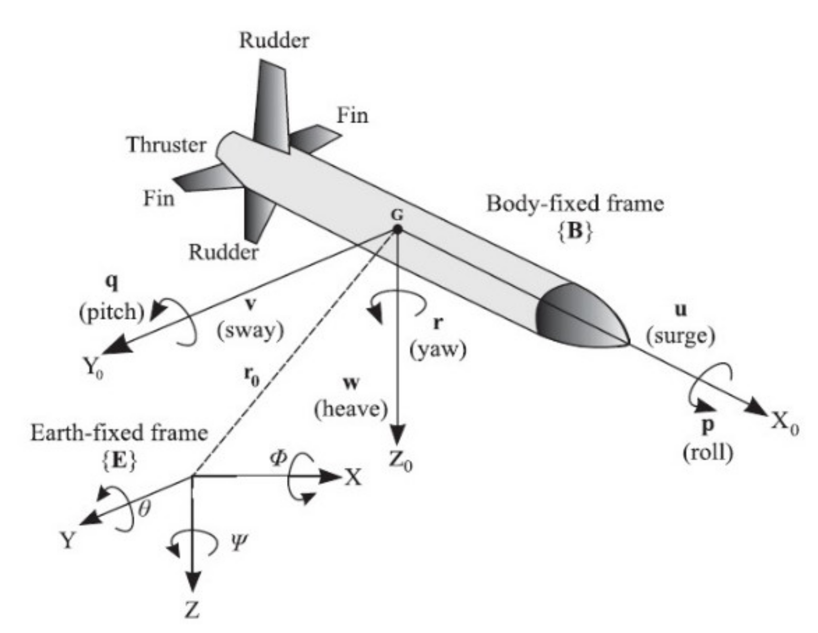
2. Dynamic System of AUV

Although the algorithm we studied is not based on the AUV dynamic model, the AUV dynamic model will be used in the following simulation and comparison with the traditional control method. The AUV dynamic model has been studied extensively [12]. The body-fixed coordinates depict AUV motion in 6-DOF, i.e., surge, sway, heave, roll, pitch, and yaw (heading) as shown in Figure 1. The mathematical models for the motion of underwater vehicles are expressed by the triple translation Equations (1)–(3) and the triple rotation Equations (4)–(6). Notations adopted are summarized in Table 1 and Table 2.
m [ u ˙ υ r + q w x g ( q 2 + r 2 ) + y g ( p q r ˙ ) + [ z g ( p r + q ˙ ) ] = X ext
m [ υ ˙ w p + u r y g ( p 2 + r 2 ) + x g ( p q + r ˙ ) + [ z g ( q r p ˙ ) ] = Y ext
m [ w ˙ u q + υ p z g ( p 2 + q 2 ) + x g ( r p q ˙ ) + y g [ z g ( r q + p ˙ ) ] = Z ext
I x x p ˙ ( I z z I y y ) q r I x x ( r ˙ + p q ) + I x y ( p r q ˙ ) + I y z ( r 2 q 2 ) + m y g y c ( w ˙ + υ p u q ) m z g ( υ ˙ + u r w p ) = K ext
I y y q ˙ ( I z z I x x ) p r I y z ( r ˙ p q ) I x y ( p ˙ + q r ) + I x z ( p 2 r 2 ) m x g ( w ˙ + υ p u q ) + m z g ( u ˙ υ r + w q ) = M ext
I z z r ˙ + ( I y y I x x ) p q I x z ( p ˙ q r ) I y z ( q ˙ + p r ) I x y ( p 2 q 2 ) + m x G ( υ ˙ + u r + w p ) m y g ( u ˙ υ r + w q ) = N ext
The kinematic model of AUV can be expressed in terms of the relative surge and sway velocities by considering the influences of the ocean currents as follows:
ψ ˙ = r x ˙ = u r c o s   ψ v r s i n   ψ + V x y ˙ = u r s i n   ψ + v r c o s   ψ + V y
where Vx and Vy are the velocity components of the time-varying ocean currents in the x and y directions of the inertial reference frame and ur, vr, and r are the relative surge, sway, and yaw velocities, respectively.
In this study, the design of the horizontal plane path tracking control of the AUV is taken as an example. The dynamic model of AUV in the horizontal plane can be simplified as shown in Equation (8) below:
u ˙ r = f u u r , v r , r + g u X T + d u v ˙ r = f v u r , v r , r + d v r ˙ = f r u r , v r , r + g r δ + d r
where du, dv, and dr denote the compound uncertainties with unknown upper bounds, XT is the propeller thrust force along the surge motion of the vehicle, is the angle of the yaw rudder δ, fu (ur, vr, r), fv (ur, vr, r), fr (ur, vr, r), gu, and gr are known nonlinear functions, as shown in Equations (9)–(13).
f u u r , v r , r = m v r r + m x g r 2 + m y g r ˙ + X u u u r u r + X u u ˙ r + X v r v r r + X r r r 2 ) / m X u
g u = 1 / m X u
f v u r , v r , r = ( m u r r + m y g r 2 m x g r ˙ + Y v v v r v r + Y r r r r + Y v v ˙ r + Y r r ˙ + Y u r u r r + Y u v u r v r ) / m Y v ˙
f r u r , v r , r = ( m x g v ˙ r + u r r + m y g u ˙ r v r r + N v v v r v r + N r r r r + N v v ˙ r + N r r ˙ + N u r u r r + N u v u r v r ) / I z z N r ˙
g r = N u u δ r u 2 / I z z N r
The 3D path tracking control mainly decouples the control into horizontal (horizontal) and vertical (vertical) ones. We design the AUV horizontal path tracking motion as an example. The path tracking control system for AUV in the horizontal plane is shown in Figure 2. The definitions of the main parameters of the AUV model are given in Table 2.

3. Design of AUV Motion Control Algorithm

The AUV motion control algorithm is used to autonomously maintain the course of the underwater vehicle. It has periods of course changing and course keeping. During the period of course changing, the motion controller rapidly narrows the course error according to the given course; while during the period of course keeping, the controller must overcome the influences of marine conditions and keep the vehicle steady and sail on a predefined course.
Some algorithms for AUV motion control have been studied. PID control strategy [13] is the widely used approach for AUV motion control. However, PID autopilot lacked the adaptability to the change of the working state and environment, so it is hard to achieve optimal control since the parameters have to be set manually. Sliding mode control strategy [14] has been proved to be able to tackle system uncertainties and external disturbances with good robustness. Thus, it is usually used for dynamic tracking control of AUV. However, one major disadvantage is the high frequency of chattering. This high-frequency chattering can cause high heat losses in the system and premature wear in thruster. Self-adaptive control [15] has certain adaptability to the change of the working state and environment of the AUV, and can automatically adjust the control parameters. However, self-adaptive control algorithm is based on the accurate mathematical model, while the actual motion process changes with the working situations and navigational environments. Thus, this is a process of time varying, nonlinearity, and large interference for a model. The control therefore cannot avoid problems, such as difficult adjustment of controller parameters, and robustness. Backstepping control [16] has been used in mobile robot tracking control and is also adapted to AUV. The idea of a backstepping algorithm is to define velocity controller that stabilizes the closed-loop system. It can deal with large initial state errors. However, sharp speed jump occurs with sudden tracking errors.
The design of an AUV motion control system implemented from classical and modern control theories usually need to know the linear and nonlinear mathematical models of the controlled object. However, AUV has high nonlinearity and uncertainty, and therefore it may be hard to describe using accurate mathematical models. Thus, the system faces a great difficulty in adopting either the classical or the modern control theory to design an ideal controller. An intelligent control system does not rely on the mathematical model of the controlled object, and has a certain adaptive capacity to the nonlinearity and time variability of the controlled object. Therefore, such an adaptive system can be applied to the nonlinear, time-varying, hysteretic, and uncertain autonomous underwater robotic motion control environment. The latest studies on developing intelligent control systems have improved the development of AUV intellectualization. The fuzzy control approach is employed for controlling uncertain or strongly nonlinear systems without knowing the precise system model. It does not need the computation procedure to be relatively simple. The underwater robots “Ocean Voyager” and “APPA”, developed by the Florida Atlantic University, both adopt fuzzy systems for depth control. For the fuzzy control adopted by the “Ocean Voyager”, the heading, trim, and depth are well controlled. Each subsystem has three controllers which are respectively designed for dealing with different velocity ranges. Additionally, the control variable of the rudder angle is a function of the input error and the velocity of error, which have good control effect. The fuzzy control system is easy to design, has good stability, and is also applicable to a nonlinear system for which constructing an accurate mathematical model can be difficult. Therefore, fuzzy control systems are useful for the development of AUV control systems [17,18,19,20]. The neural networks control method is also used widely in controlling dynamic systems. No exact vehicle model is required and AUV’s nonlinearities can also be well implemented. Some literature works [21,22,23,24,25,26,27,28] propose to apply neural network controllers to the control of underwater robots. Neural network-based control is a type of control method that conducts simulation by using features such as distributed storage, parallel processing, and adaptive learning, adapted from a biological neural system. The feature of AUV motion control requires that it has a wide working range (e.g., velocity change range, and working range), which makes neural networks suitable for application in this field.
Fuzzy control is an effective method to solve the uncertainty problem in system control. A fuzzy control system is highly robust against the influence of interference and parameters changes. However, the absence of a learning function is a big disadvantage for a fuzzy control system. Neural networks have strong self-learning and fault-tolerance abilities. By introducing these learning mechanisms of neural networks into the fuzzy control system, and using the fuzzy information to train neural networks, the system can be developed to self-adjust, self-organize, and self-learn.

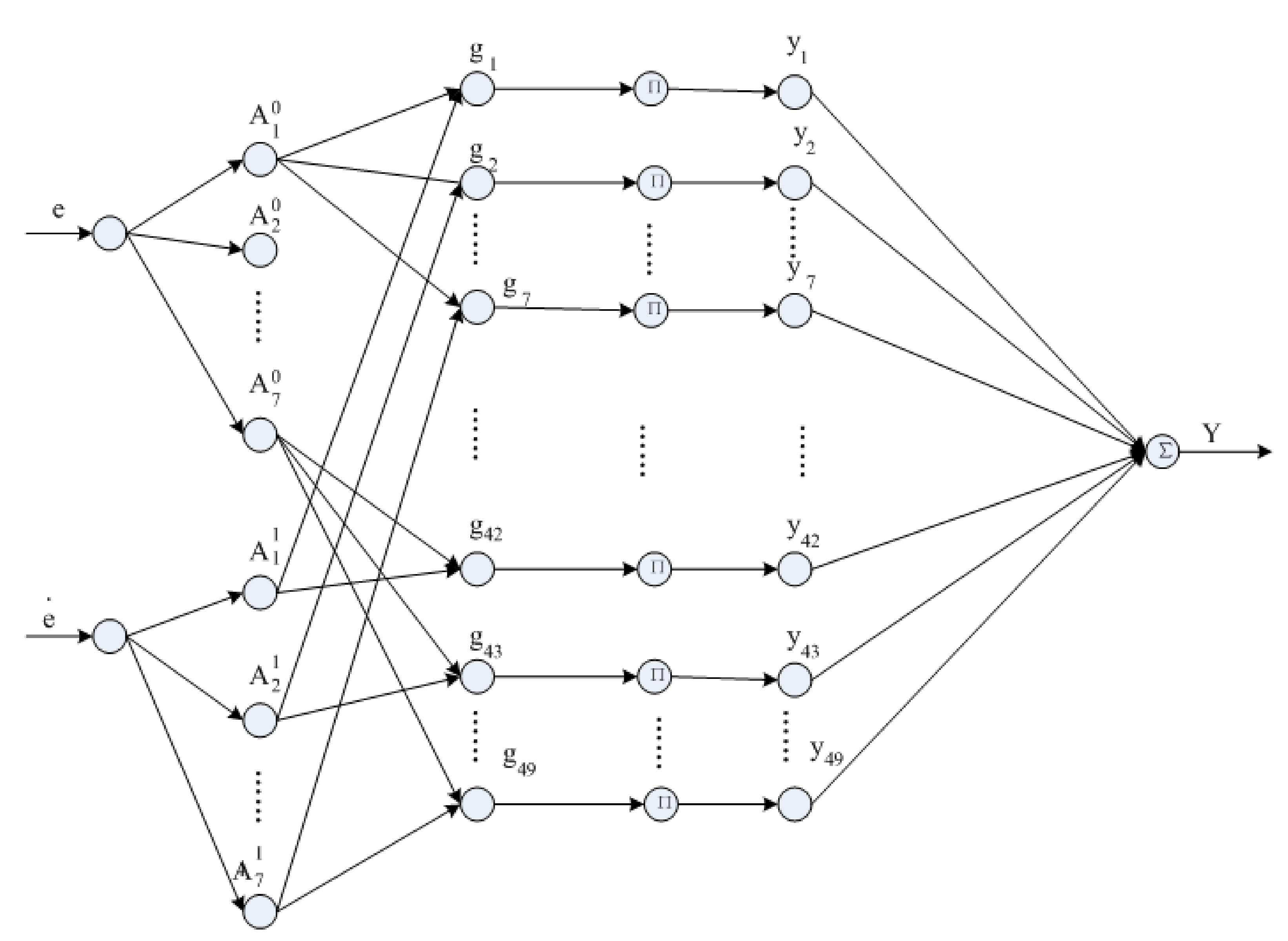
3.1. Design of Neuro-Fuzzy Controller for AUV Path Tracking

In this paper, we combine the fuzzy control system with a neural network to design the T-S fuzzy neural network for AUV tracking control. The “IF” part of the fuzzy rule of T-S model is similar to the “IF” part of Zadeh’s rule, but its “THEN” part is an exact function, usually an input variable polynomial. In the conclusion part of the T-S fuzzy inference model, a linear local equation is used to replace the constant in the general inference process. Therefore, the T-S model can generate complex nonlinear functions with a small number of fuzzy rules, which can effectively reduce the number of fuzzy rules when dealing with multivariable systems, so it offers great advantages. The nonlinear mapping and learning characteristics of a neural network with approximate ability can well solve the difficulty of the uncertainty of the dynamic parameters for an underwater vehicle.
We design the path tracking control algorithm for the AUV path tracking. Now, taking the AUV horizontal path tracking motion, a T-S neuro-fuzzy controller is designed. The neuro-fuzzy controller is made up of an antecedent network and a consequent network. The consequent network dynamically adjusts the rule library. The antecedent network consists of five layers: (a) input layer, (b) fuzzification layer, (c) inference layer, (d) normalization layer, and (e) output node layer. In this network, the excitation function (input membership function) at the fuzzification layer adopts a Gaussian function, and the antecedent network makes online adjustments to the position and width of the input membership function, as shown in Figure 3.
The AUV course tracking controller designed in this paper is double-input and single-output, with two input variables e ,   e ˙ which, respectively, represent the course deviation e , and the change rate of the course deviation e ˙ . The single output variable y represents the rudder order. The control rules can be expressed as the following analysis formula:
y = < α e + 1 α e ˙ >
Generally, there are different requirements for the weighting degrees of error e and of the velocity of error e ˙ . For the two-dimensional fuzzy control system, when the system error is rather large, the main task of the control system is to eliminate this error. At that moment, it needs to give a larger weight to the error control process. The larger the error, the larger the weighting of the process will be. Otherwise, when the error is rather small, the system approaches a steady state, and the principal task of the control system makes the system stable as soon as possible by reducing overshoots. Thus, in this case, the error change should play a larger role in the control system and it conducts a larger weighting towards error change.
According to the rules above, the adjustment factors are changed to be adjustment function   α t , and it is advisable to use the error and absolute value of the error change itself as the weighting of itself. In addition, it should satisfy the condition of the weighted sum of both being equal to be 1. The function of the error and weight function of the error change are shown as below in Equations (15) and (16):
α e t   =   e t / e t + e ˙ t
α e ˙ t   =   e ˙ t / e t + e ˙ t
where, e t and e ˙ t are the normalized deviation and deviation ratio of the AUV at the current time, respectively. The weight function shown above is merely the function of the input variable with the control strategy of the artificial intelligence and is called the weight function of intelligence. The weight function of intelligence is adopted to weight the error and the error change to obtain the following fuzzy control rules:
R s : if e = A i and e ˙ = B j , then
y = e t e t + e ˙ t A i + e ˙ t e t + e ˙ t B j i , j = 1 , 2 , , 7
where, A i and B j are the values of the deviation and the deviation variation rate in the initialization rules library, respectively, and y   is the output value corresponding to the new fuzzy rules.
For the control rules described by the analytical form above, in each control node, the list of fuzzy rules is dynamically generated according to the actual deviation and the deviation change rate. It is not restricted to the quantization level of the output variable. By an online adjustment of the control rules, the system generates excellent performances with a rapid response and a highly stable accuracy.
This network adopts a standardized five-layer network structure and a corresponding set of (7 × 7 = 49) fuzzy rules. These rules have two input variables and one output variable, which are the propeller thrusts (torques) for each degree of freedom. The domain of the input and output is {−6, −5, … −1, 0, 1 …5, 6}, which are the fuzzy membership functions of the system adopting a Gaussian function.
The input and output relationships at each layer are listed as below:
The first layer (the input layer): This layer has two nodes, and is used to input the transformed error e and the error change rate e ˙ into the network. It only transfers the signal and does not process it.
f i ( 1 ) = x i ( 0 ) ; y i 1 = x i 1 i = 1 , 2
The second layer (fuzzification layer): In the node function
f i j 2 = e ( x i 2 c i j ) 2 / σ i j 2 ,
The node accepts the input layer signals and uses a Gaussian function as the membership function to divide the distribution of the input signals. In the formula, c i j and σ i j 2 are respectively the central and width value parameters of the Gaussian function.
x i 2 = y i 1
y i j 2 = e ( x i 2 c i j ) 2 / σ i j 2 i = 1 , 2 ; j = 1 , 2 , , 7
The third layer (inference layer): Each node at this layer represents a single rule, with the 49 nodes in total representing 49 distinct rules. Each inference rule adopts the AND operator. The node function is represented as:
f i j 3 = m i n { x 1 i 3 , x 2 j 3 , 1 }
x i j 3 = y i j 2
y k 3 = m i n { x 1 i 3 , x 2 j 3 , 1 }
k =   i 1   ×   7 + j i = 1 , 2 , , 7 ; j = 1 , 2 , , 7 ; k = 1 , 2 , , 49
The fourth layer (normalization layer): This layer performs the normalization processing on the inference result of each rule. The node function is represented as:
f j 4 = x j 4 / i = 1 m x i 4
x k 4 = y k 3
y k 4 = x k 4 / i = 1 49 x i 4 k = 1 , 2 , , 49
The fifth layer (output node layer): All the nodes in the normalization layer connect with this layer to finish solving the ambiguity. The weight w j of each connection represents the central value of the output membership function for each rule. This layer has only one output, that is, the control force (torque) on the principal axis of the AUV.
x j 5 = y j 4
y 5 = j = 1 49 w j x j 5 j = 1 , 2 , , 49 ;
The weight w j in the Equation (30) is substituted by the output value of the consequent network’s corresponding node. The error function E W for this is represented as:
E W   = 1 2 ( y d y 5 ) 2 = 1 2 ( y d j = 1 49 w j x j 5 ) 2 = 1 2 e 2
where, y d and y are the desired output and actual output, respectively. Now, the error back-propagation algorithm is presented to adjust the location c i j and the width σ i j of the membership degree function. E / c i j and E / σ i j are calculated, and then the first-order gradient optimization algorithm is used to adjust the values of c i j and σ i j .
Then, the error value is calculated as
ε 5 = E f 5 = E y 5 = y d y = e
The fifth layer weight w j ( j = 1 , 2 , , 49 ) is substituted by the output value of the nodes corresponded by consequent network. The error is propagated back to the fourth layer to obtain the normalization layer:
ε i 4 = E y 4 = E y 5 y i 5 x i 5 x i 5 y i 4 = ε 5 w i j = 1 , 2 , , 49
The calculation of inference error layer is performed as follows:
ε j 3 = E y j 3 = E y j 4 y j 4 x j 4 x j 4 y j 3 = ε j 4 i = 1 i j 49 x i 3 / ( i = 1 49 x i 3 ) 2
ε j 2 = E y j 2 = k = 1 7 E y k 3 y k 3 x i j 3 x k 3 y i j 2 = k = 1 7 ε k 3 S i j e y i j 2 = k = 1 7 ε k 3 S i j e ( x i c i j ) 2 σ i j 2
where a minimization operation is performed on y 3 such that y 3 x i j 2 = μ i j is the minimum value output by the kth rule node:
S i j = y k 3 x i j 3 = y k 3 μ i j = 1
Otherwise:
S i j = y k 3 x i j 3 = y k 3 μ i j = 0
Thus, the first-order gradient is obtained as follows:
E c i j = E f i j 2 f i j 2 c i j = ε i j 2 2 x i c i j σ i j 2
E σ i j = E f i j 2 f i j 2 σ i j = ε i j 2 2 ( x i c i j ) 2 σ i j 3
After the required first-order gradient is obtained, the parameters are finally used to adjust the learning algorithm:
W k + 1   = W k β E ( W k W
c i j k + 1   = c i j k β E c i j
σ i j k + 1   = σ i j k β E σ i j
where, i = 1 , 2 , , 7 ; j = 1 , 2 , , 7 ; β > 0 forms the learning rate.
We have completed the design of the neural network structure, and the training process is shown in Figure 4. The output of the traditional neural network is only determined by the input value and the connection weight between the input layer and the hidden layer in the latter network. If some characteristic component data are lost, distorted, or saturated in the input data, the output value of the hidden layer node of the traditional back-component network may fluctuate largely, resulting in the loss of the discriminant ability of the network.
In this paper, the system considers the effect of fuzzy membership degree of each feature component on the generation rule of output. In this way, the effect of interference on the output can be reduced or even ignored. In the fuzzy rules corresponding to all kinds of sample sets generated by clustering, the output value does not vary considerably.
It can be seen that the improved fuzzy rule can suppress and eliminate the feature components in samples that do not belong to this category, which can greatly enhance the robustness of the model.
The control system based on neural networks uses a neural network to realize the fuzzy system, applying the learning function of the neural network to the fuzzy system, and enables the fuzzy system to automatically adjust and obtain the fuzzy rules from the learning. If there is a wrong sample training network, after the normalization of traditional network, only one or several rules Wj with a very small value and the largest value are selected to activate the node and produce output. This hinders the traditional network from retaining the local response characteristics of the neural network properly. There is a slow convergence of the network, so a local optimal situation can occur. In the improved network, although normalization is also adopted to improve the generalization ability of the model, the output of error samples can be effectively suppressed in the generation process of fuzzy node output, corresponding to fuzzy rules. This greatly increases the local response ability of the model.

3.2. Optimization and Analysis of Controller Parameters

In the design of the network, we consider several parameters such as the number of layers of the network, the number of neurons in each layer, the activation function, the initial value, and the learning rate. The following are its selection principles:
(1)
The number of layers in the network
It has been proved in theory that a network with deviation and at least one S-shaped hidden layer plus one linear output layer can approach any rational function. Increasing the number of layers can further reduce the error and improve the network accuracy, but at the same time, it also complicates the network. In this study, we used a four-layer neural network.
(2)
Number of hidden layer neurons
The improvement in the training precision of the network can be obtained by using a hidden layer and by increasing the number of neurons in it. This is much simpler in terms of structural implementation than increasing the number of layers in the network. We use the accuracy and time required to train the network for measuring the quality of a neural network design:
(a)
When the number of neurons is too small, the network cannot learn efficiently, the number of training iterations is relatively large, and the training accuracy is low.
(b)
When the number of neurons is too large, the more powerful the network function, the higher is the network accuracy, and the number of training iterations is also large, which may result in overfitting. Therefore, depending on the accuracy of the AUV heading error, we divide them into seven levels, so the number of neurons in the hidden layer is seven.
(3)
Selection of the initial weights
In general, the initial weight is a random number between (−1, 1). The initial weight of a neural network design is assigned random decimal numbers that are unidentical to those generated by a random generator.
(4)
Learning rate
Generally, the learning rate is between 0.01 and 0.8. A large learning rate might lead to instability of the system, whereas a small learning rate might lead to slow convergence and would require a longer training time. For highly complex networks, different learning rates might be required at different locations of the error surface. In order to reduce the training times and the time required to search for the learning rates, an efficient method would be to adopt the adaptive learning rate of variation to set different learning rates at different stages. On the basis of debugging, we designed the adaptive transformation of the learning efficiency according to the heading error. When the heading error is greater than 10°, the learning rate is 0.6; when the heading error is greater than 5°, the learning rate is 0.3; and when the heading error is less than 5°, the learning rate is 0.1. Experiments show that adaptive adjustment of the learning rate can accelerate convergence and avoid overshooting.

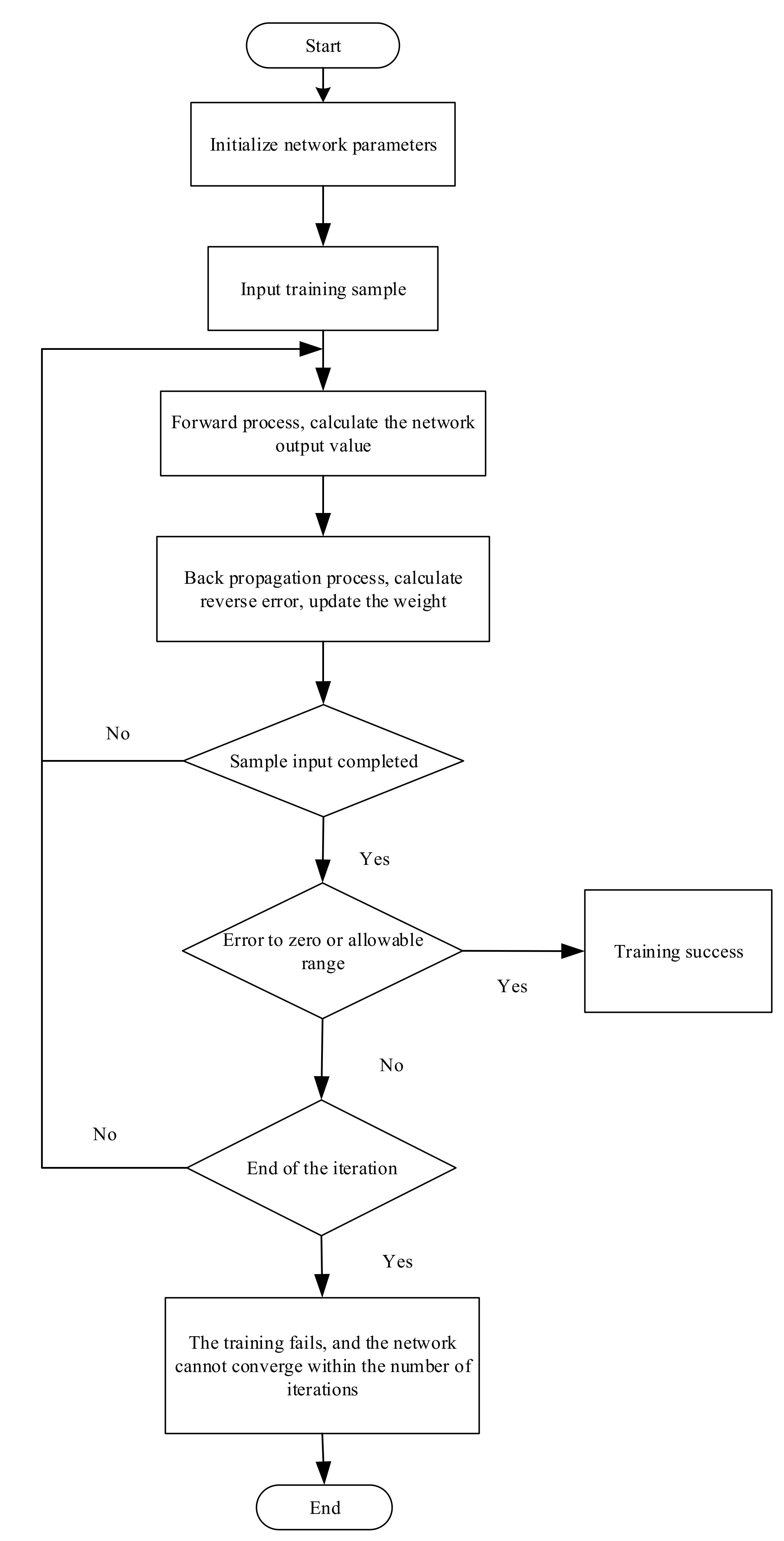
3.3. Convergence Analysis

Hypothesis 1.
(i) 
There is a constant such that for any i = 1 , 2 , , n , k = 1 , 2 , m , there is:
a 0 k C 0   , a i k C 0 , b i k C 0 ,
(ii) 
There is a set D 0 for W k k = 0 D 0 , and a set H = W D 0   : E W W = 0 , that contains only a finite number of points.
Theorem 1.
(i) 
Let the error function E(W) be defined by Equation (31). Starting from the initial point, {wk}, is the weight sequence of the network is obtained by Equation (40). If hypothesis (i) is satisfied, then E W k + 1 E W k ,   k = 0 , 1 , 2 , ; lim k E W k W = 0 .
(ii) 
If hypothesis (ii) is also true, then there is a point W * that makes
(iii) 
lim k W k = W * .
Conclusion (i) in Theorem 1 shows that the E(W) decreases monotonically during training. Conclusion (ii) shows the weak convergence of the weight sequence {wk}, i.e., starting from any point W0 in the weight space and updating the weight according to Equation (40), the weight sequence, {wk}, obtained satisfies Equation (40). Conclusion (iii) shows that the number of stable points on the error function surface is limited, and thus the weight sequence must converge to a local minimum. Hypothesis 1 indicates that the conclusion of the theorem requires an a priori condition, i.e., the bounded nature of the weight sequence in the training process. This assumption is also necessary for the convergence analysis of the gradient training algorithm of an ordinary neural network.

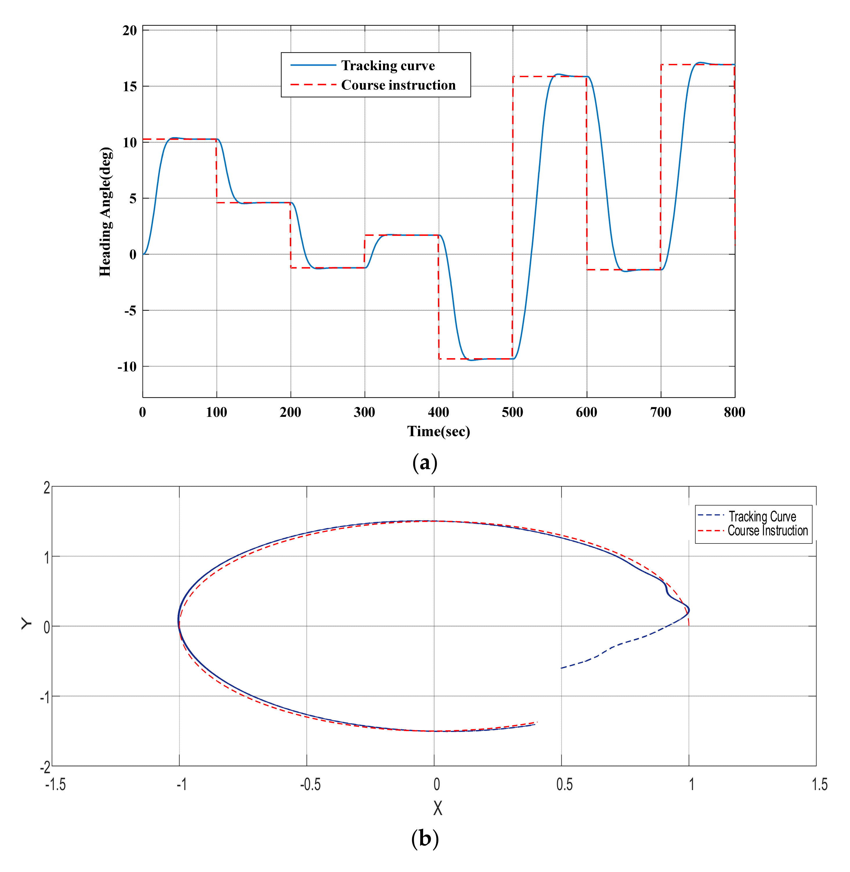
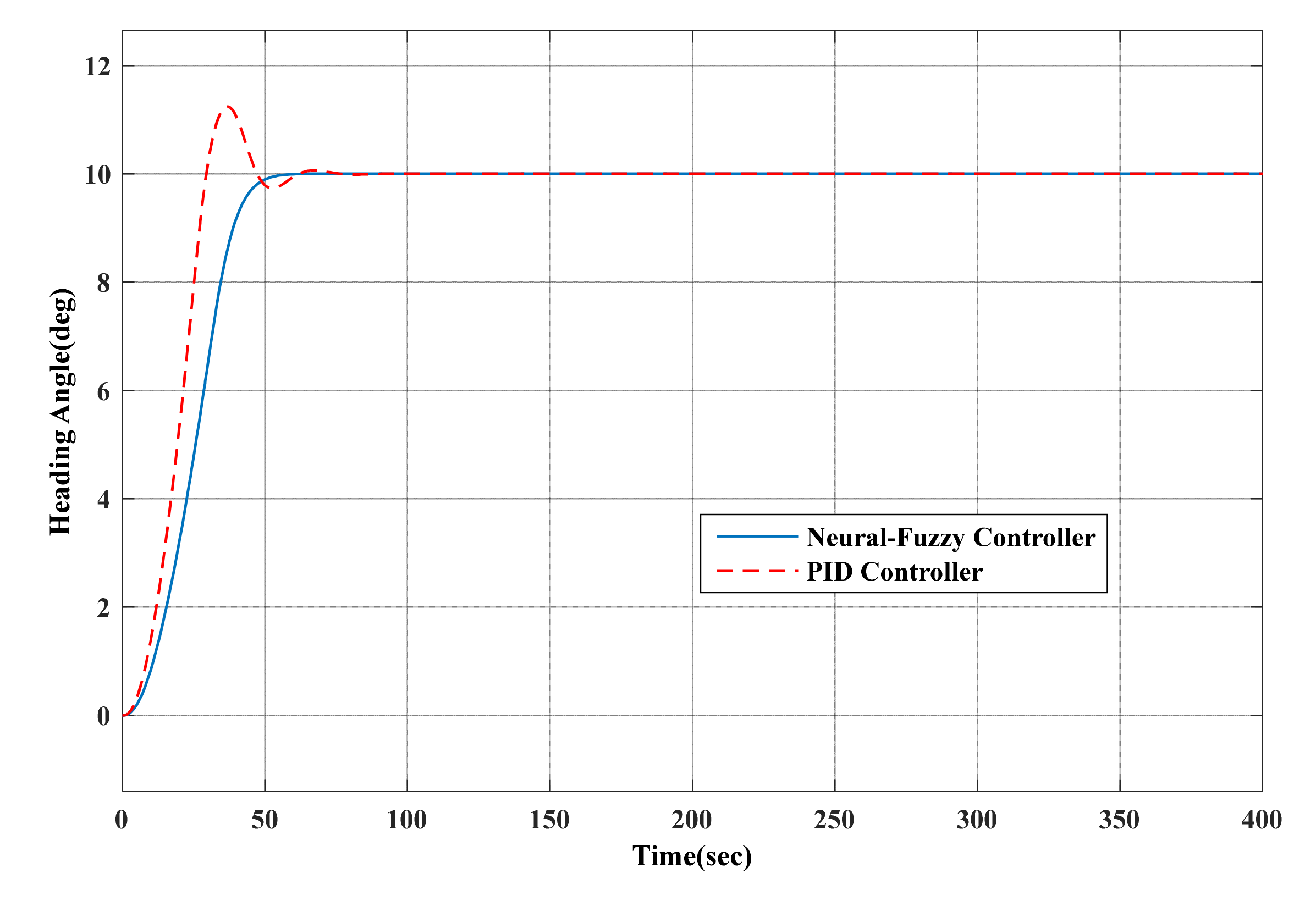
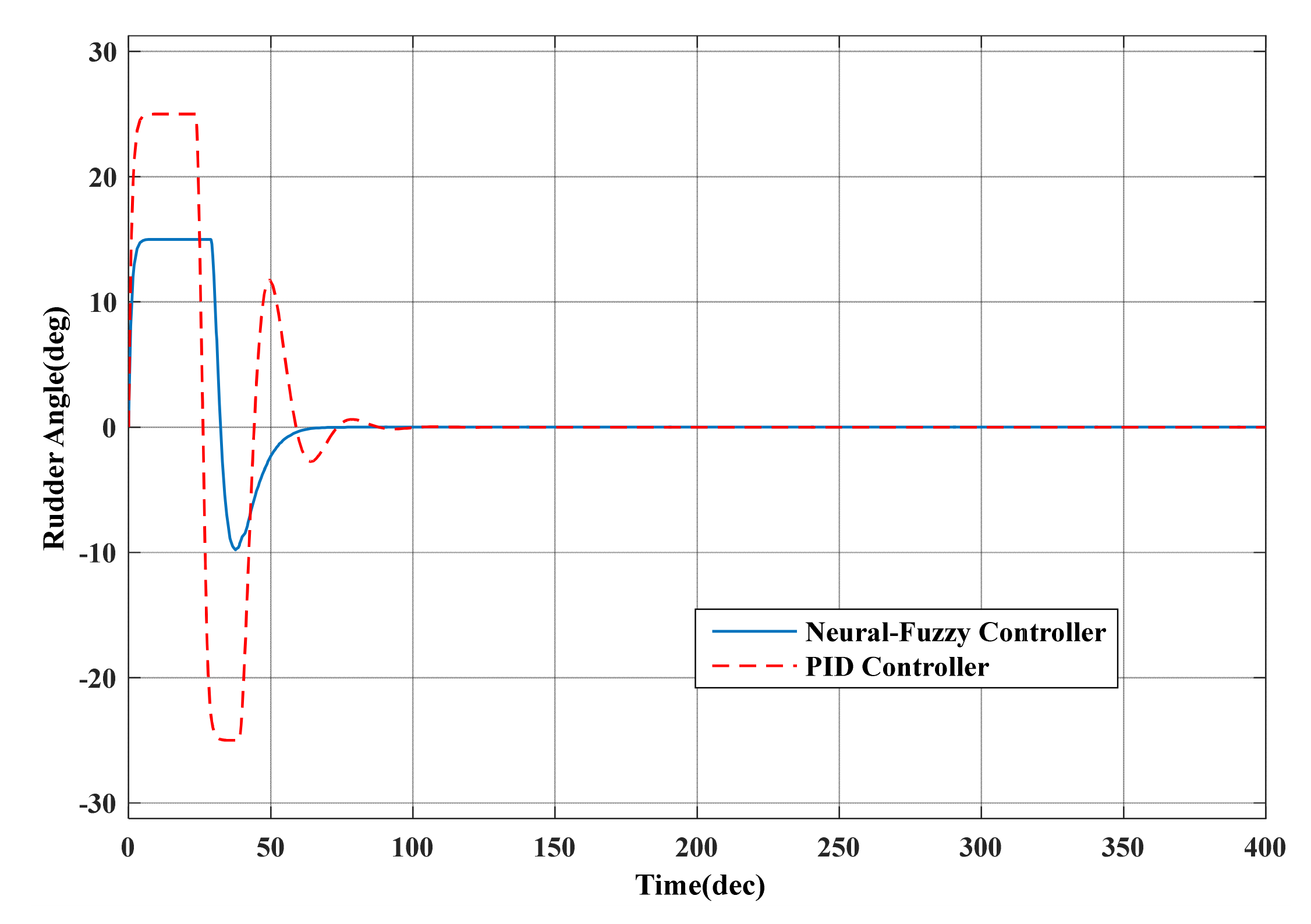
3.4. MATLAB Simulation

The MATLAB software is used to simulate the course control system. The performance goals of the AUV motion control system are: (1) during the period of course changing, the motion control system changes the course rapidly and steadily, realizing a short accommodation time to not overshoot from the path; (2) during the period of course keeping, the motion control system must be able to eliminate interferences, and maintain robustness towards the model perturbation. In the control system, we established an AUV mathematical model according to the above AUV dynamics formula, and the important parameter settings are shown in Table 3.
We introduce the reference trajectory setting technique used to design the reference course signal. To prove that the capacity of the controller in the design is capable of resisting external interferences, the sea wave interference model is imposed on the AUV model. Figure 5 shows the course tracking signal. The simulation results show that the course output can be rapidly changed to reach a predefined value such that the control response is smooth and the overshooting is small. The goal is to create an ideal tracking effect of the controller to match the course. From the simulation results, we can see that the course change is rapid and steady and has no static error.
Simulation results in Figure 6 show the comparison between the designed neuro-fuzzy controller and the adjusted PID controller. After a perturbation of 80% to the model parameter, a large overshoot occurs in the PID system. Figure 7 demonstrates the robustness of the neuro-fuzzy controller design by showing that the control effect works smoothly even after perturbations affect the model. Figure 4 shows the rudder order outputs of the neuro-fuzzy controller and the PID controller. When the course deviation is large, the two controllers output a large helm angle to reduce the course error. When the course deviation decreases, the rudder angle is reduced and finally a small counter rudder is output so that the vehicle avoids overshooting. The designed neuro-fuzzy controller has a lesser number of rudders and a lower rudder angle than the PID controller. Thus, the designed controller has better performance.

4. Development of the AUV Motion Control Virtual Reality System
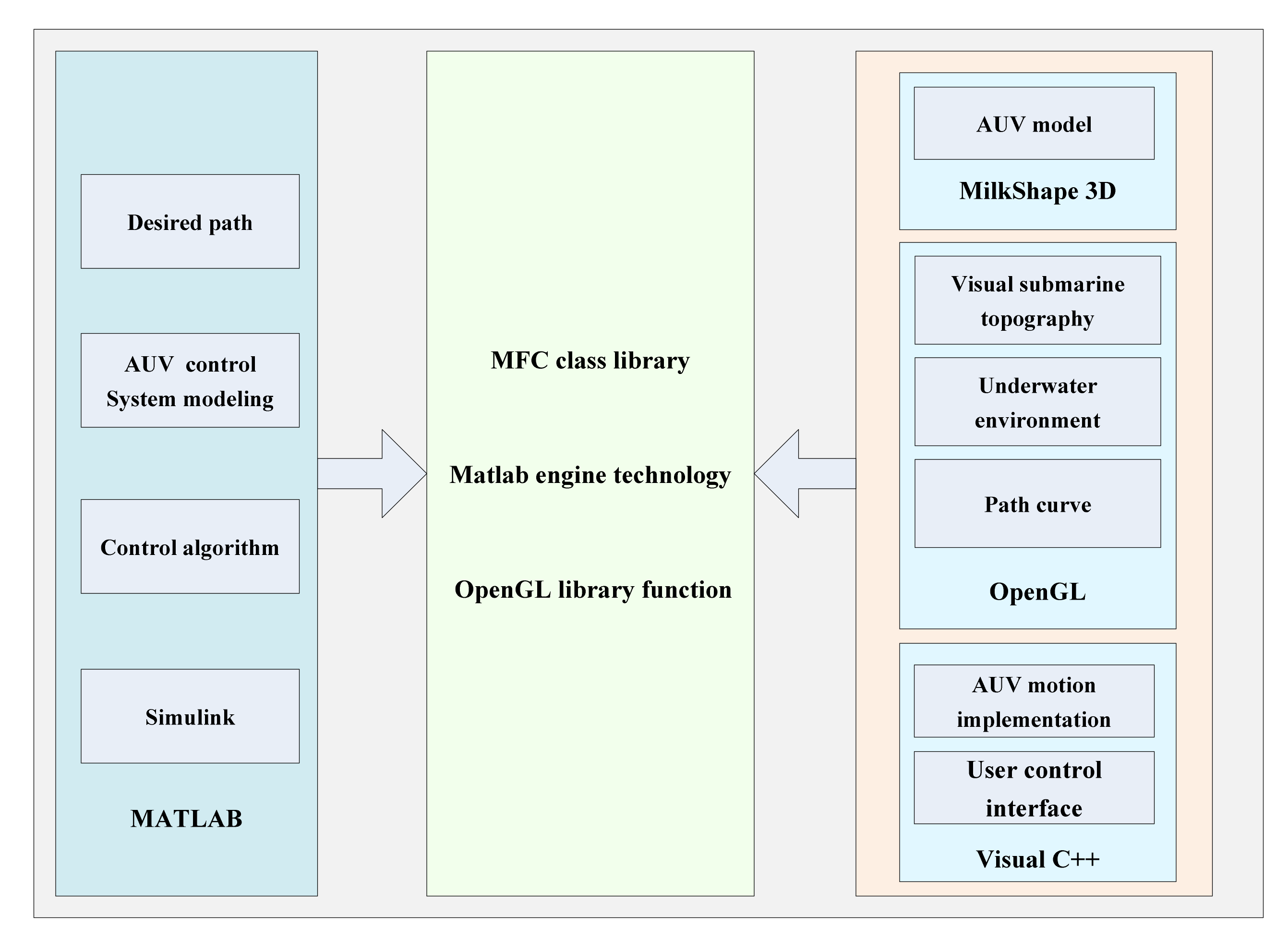
4.1. Overall Design

Before development of the virtual design, one needs to consider the tasks the system should perform, such as showing vivid virtual scenes, changing scene element attributes according to demand, and obtaining numeric parameters of scene elements in real time. The development task of designing the system comprises of three parts:
  • Construction and display of 3D AUV and virtual environment scene: A 3D modeling software is used to generate the AUV 3D model and other environmental element models. Each element is appropriately deployed to generate a 3D virtual scene of underwater robotic motion.
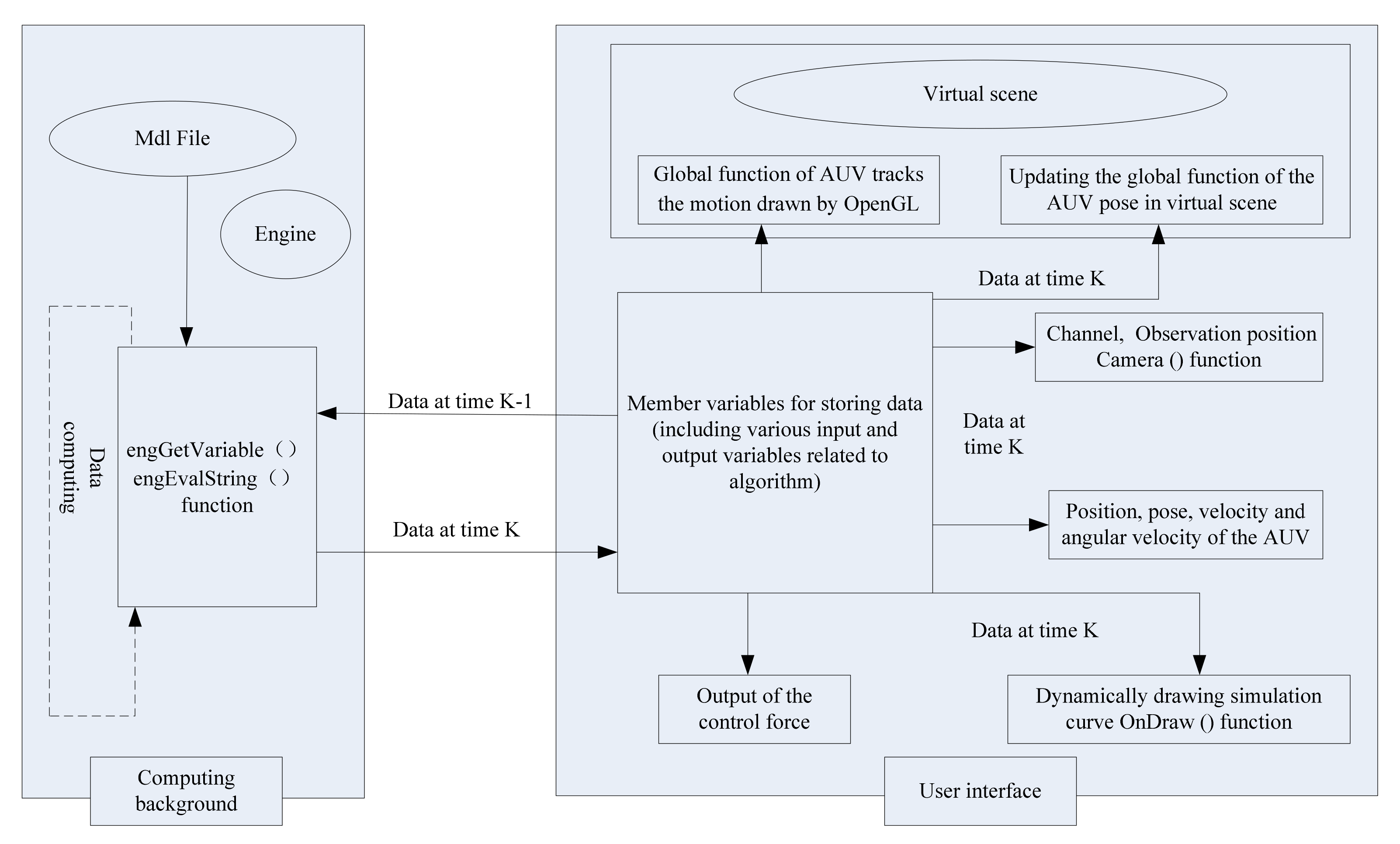
  • AUV motion control realization and output display: This paper provides two methods for the realization and output of the AUV motion control. The first method directly uses Visual C++ programming in the virtual reality system to realize the AUV motion control algorithm and displays the results on the AUV motion visual simulation interface. In the second method, the system first uses MATLAB to design the AUV motion control algorithm, and then uses the MATLAB engine to execute the commands and perform the data transmission between MATLAB and the virtual simulation system under the Visual C++ environment. The output of the AUV motion control system designed using MATLAB can be shown in the virtual reality system.
  • Design of AUV motion control virtual reality system: The key functionalities of a virtual reality system are a) how to “control” the virtual scenes, b) how to integrate and synchronize the AUV motion control and virtual scene under the same software platform, and c) how to realize the poses of the AUV 3D model motion and the “communication” of the control algorithm.
The choice of the software used for the development of the virtual reality system is as follows: (a) MilkShape 3D: The 3D model drawing software can flexibly call the OpenGL (open graphics library) library for drawing. (b) MATLAB: MATLAB has powerful operational capabilities and can implement complex AUV motion control algorithms, such as neural networks and fuzzy control. (c) Visual C++: Visual C++ combines many development tools together as an integrated development platform.

4.2. The Framework of AUV Motion Control VR System

The AUV motion control virtual reality system can simulate difference functions, such as desired path setting, AUV modeling, marine virtual scene modeling, and ocean current interference model establishment. It can perform these simulations at different viewing angles of the AUV motion, to create dynamic displays of motion curves, and provide real-time data display to output the simulation results. The different components of the system were developed using a combination of programming languages and software platforms. Visual C++ was used to design the user interface and the AUV motion display interface. MilkShape 3D and OpenGL were adopted to model the AUV and the marine environment. The MATLAB engine was used to realize the data communication between MATLAB and the AUV virtual reality system. As a computing background, MATLAB was used to conduct visual simulations of 3D space motion control for the AUV in the virtual reality system. The AUV motion control virtual reality system framework is shown in Figure 8.
The AUV virtual reality system contains seven functional modules: (1) the simulation module, (2) the AUV module, (3) the settings module, (4) the control module, (5) the display module, (6) the communication module, and (7) the help module. The simulation module forms the kernel of the AUV system. A visual simulation modeling software is used to establish the model base for the AUV and the submarine topography. The visual simulation platform of the AUV is developed using a real-time visual simulation software which performs the real-time interaction control against the AUV motion.

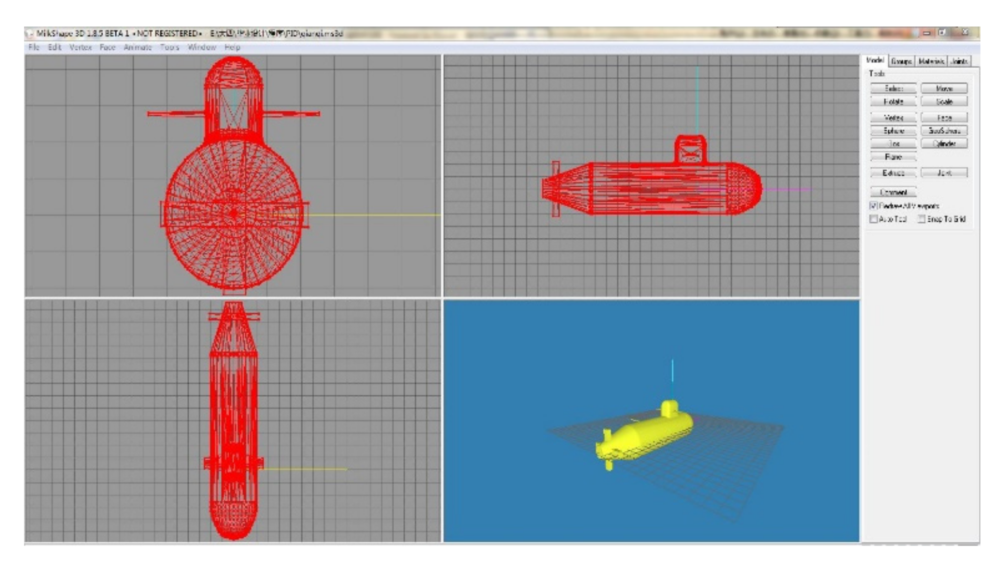
4.3. Construction of AUV Model

The AUV 3D model is the main body of the whole virtual simulation scene. The principle task is to draw a three-dimensional and vivid AUV geometric appearance in MilkShape 3D. The appearance of the AUV consists of several parts, such as the vehicle body, the pitching rudder, and the rudder. These parts are divided into nodes, body nodes, and face nodes based on their relative positions. According to the structural relationship among all the parts, the position and the angle of the coordinate surface are transformed flexibly when being drawn. Tools such as polygon, rotating, translating, zooming, and mirroring are invoked through the M ilkShape 3D drawing toolkit, and the collected texture files are mapped into the corresponding surfaces of the model framework. Eventually, the AUV model shown in Figure 9 is obtained.
The propeller, the rudder, and the pitching rudder at the tail of the AUV tail provide the control force and the torque while the AUV is in motion. This determines the changes in velocity and angular velocity. In the virtual simulation system, the moving states of the AUV should conform with the force and torque generated by the aforementioned devices.

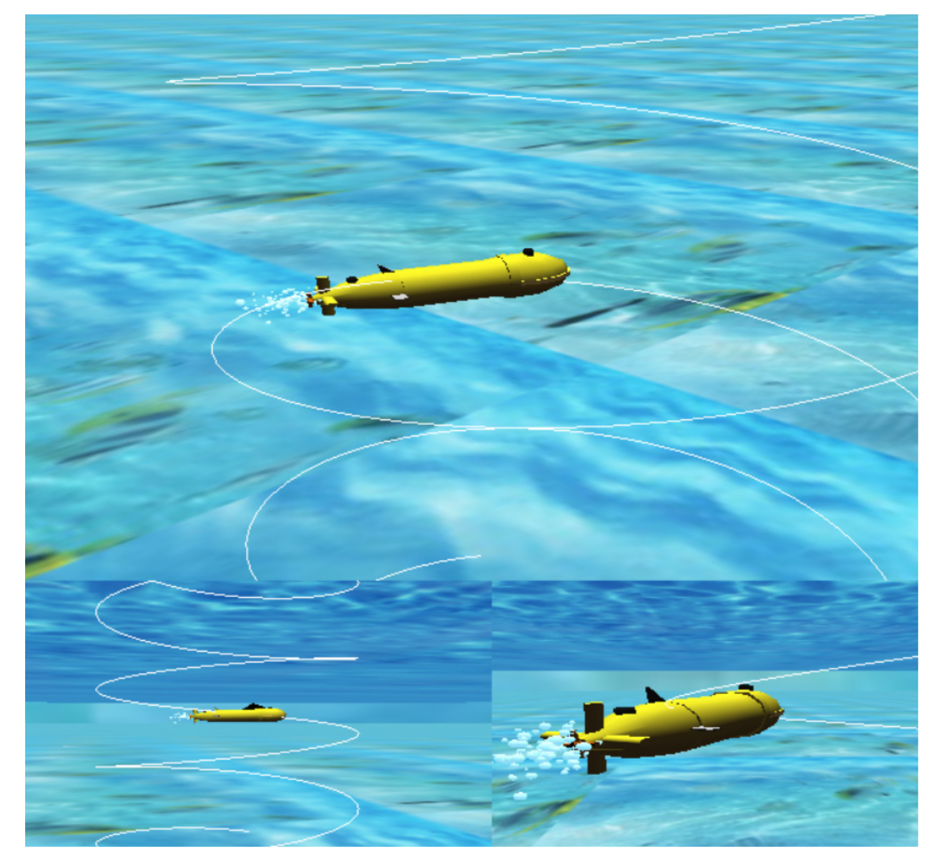
4.4. Construction of the Underwater Virtual Scene

In the AUV visual simulation system, the sea surface is an important component. The sea surface in real world is dynamic; in addition to some undulating waves, it also has mobility. Realizing this effect in OpenGL is an extremely complex work, which involves numerous calculations performed by the algorithm. In our system, we render the sea surface with mobility as shown in the generated 3D environment in Figure 10.
During scene design, the added simulation of obstacles creates a more realistic feeling of the AUV movement.
The change of the viewpoint defines the directions and positions of the objects in the scene simulating the imaging process of a camera. The effect is similar to that of putting a camera in a 3D space to record images of objects to be displayed. In an AUV visual simulation system, several cameras are defined and some necessary parameters are assigned to these cameras. These parameters can be freely selected by the users and flexibly switched to change the viewpoints and the scenes.

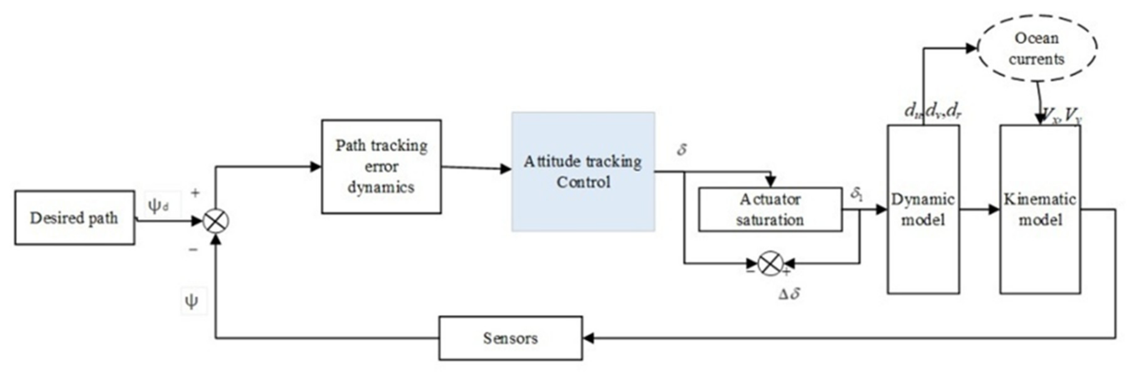
5. Data Communication between the Virtual Reality System and MATLAB

The virtual reality system proposed in this paper can directly use Visual C++ programming to implement the AUV motion control algorithm in the simulation system. Alternatively, it can first use MATLAB to design the AUV motion control algorithm and then use the MATLAB engine to implement the data communication between MATLAB and the virtual reality system under the Visual C++ environment. The algorithm is shown in Figure 10. During the simulation phase, the program calls MATLAB modules that run as background processes and updates the member variables stored as the numerical “current” time in the program.
The MATLAB computing platform and the member variables of the stored data of the virtual reality system perform bidirectional data transmissions. Let the current time be the (k−1) the time of the simulation. At this time, the Visual C++ software will initiate data transmission to the engine and perform the computation in the MATLAB system. The computation results are then outputted through the Engine library function, reassigning new values to the corresponding member variables at time k.
The motion of the AUV 3D model in the virtual scene is controlled by continuously assigning values to the position, pose angle, velocity and angular velocity member variables of the AUV. The MFC class library of the Visual C++ platform is used to define and control the motion functions of the AUV in virtual scenes.
These functions manage the member variables that represent the position, pose, velocity and angular velocity of the AUV, and use the Move function to control the motion states of the AUV 3D model. This continuous transmission of the member variables between the control algorithm and the AUV motion synchronizes the two systems. The system obtains the input value from the virtual reality system based on the Visual C++ platform, and uses MATLAB as the computing background to realize the AUV motion control algorithm, and then outputs the computing results to the virtual reality system.
The system demands that the pose changes of the AUV 3D model in the Vega scene should be consistent with the results obtained from the computing background. Likewise, the functions in the OnDraw class also rely on these member variables to complete the drawing and update the simulation curve. At the kth time, during the simulation, the functions in the OnDraw class will determine the coordinate range, draw the curve, and change the coordinate annotations according to the numerical values stored in the member variables at that time. The motion status of the AUV can be transferred to the function within the OnDraw class synchronously.

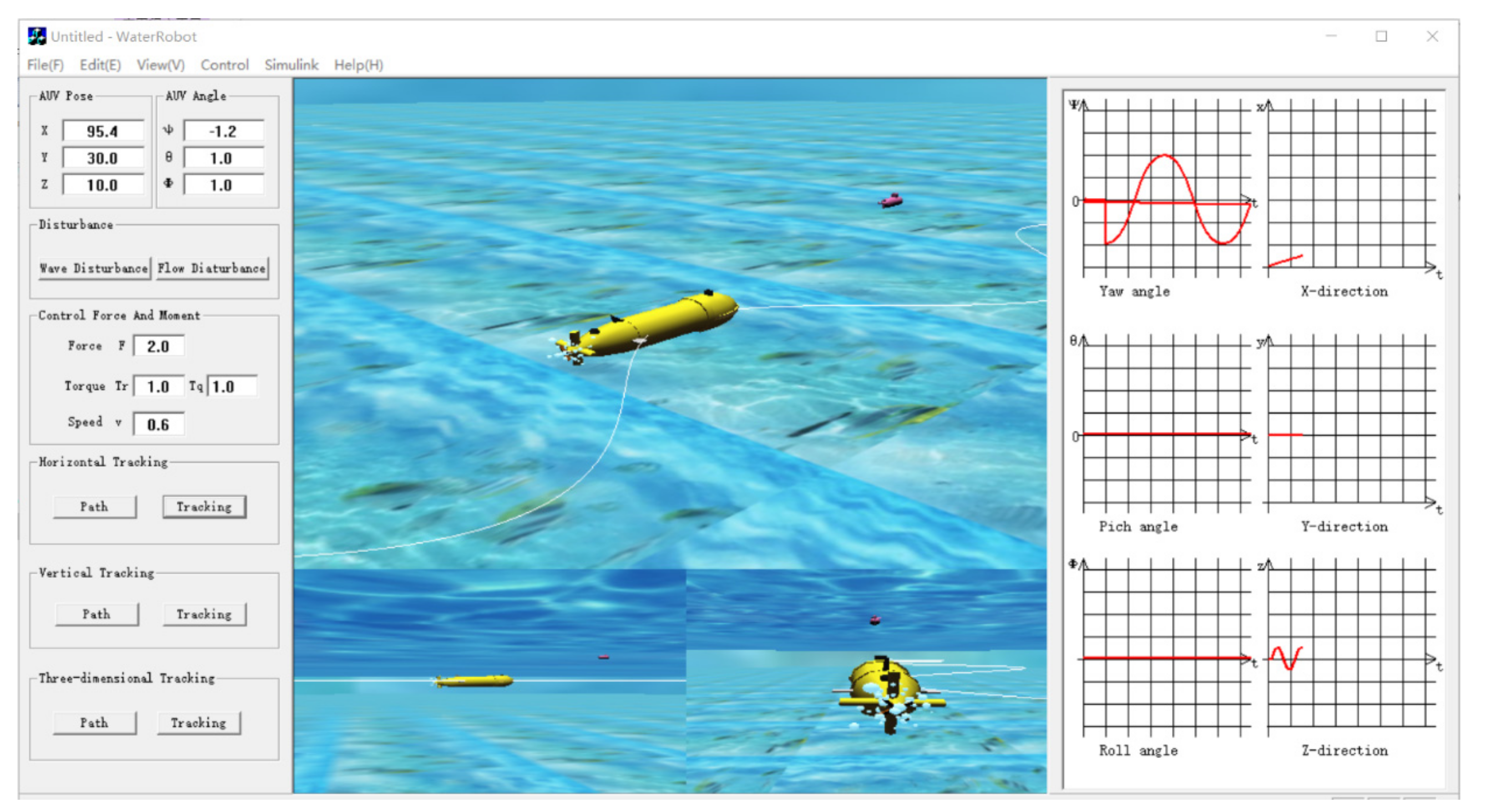
6. Visual Simulation of the Virtual Reality System

The MATLAB engine adopts a client/server based computing model. The client and the server can exist on the same computer, or can be distributed over two computers, sharing information over a network. The application uses a hybrid of Visual C++ programming and MATLAB programming, as the front-end client. The Visual C++ platform receives the data from the MATLAB engine and transmits the command and the data to the MATLAB engine. As a server, the MATLAB engine processes data at the background. In MATLAB, the following functions are used to call the MATLAB engine from the Visual C++ language: The engOpen and enclose functions are used to turn the engine on and turn off; the engGetVariable and the engPutVariable functions are used to get and send a MATLAB array from the engine; and the engEvalString function makes the engine execute the commands in MATLAB grammar.
For AUV motion control, the virtual reality system can be used to verify the effects of the motion control algorithm. The motion control simulation uses MATLAB simulations as the main operational tool. It is not intuitive to estimate the effectiveness of the algorithms just from the calculation results or the simulation curve. Therefore, in this paper, we develop a virtual simulation system with synchronous operations and perform analog and digital simulations of the AUV motion. We use intuitive visual simulation to perform tests using the neuro-fuzzy control algorithm. The AUV’s horizontal motion control is shown in Figure 11. We also design a three-dimensional motion controller in MATLAB. Then, as shown in Figure 12, the AUV virtual reality system vividly shows the motion state of the autonomous AUV. This achieves the goal of using virtual reality technology to verify the AUV motion control algorithm, not only saving the costs of voyage trails, but also providing a more intuitive and vivid interface for the design.

7. Conclusions

In this paper, virtual reality technology is applied to the development of a simulation platform for AUV 3D path tracking. This simulation platform can be utilized to observe and analyze the motion conditions of an AUV. It can also analyze the effects of the controller. A researcher can program the system to implement a motion control algorithm in the AUV virtual reality system. Moreover, this system can be utilized to design an AUV’s control algorithm in the MATLAB software environment. The output of the control system in MATLAB can drive the AUV in a 3D motion space to create a virtual simulation. Users will not see the monotonic curve anymore, but will find out the vivid motion conditions of the AUV simulation in the real environment in a virtual scene. In this paper, the AUV neural-fuzzy controller can rapidly track the course setting, to make a smooth control response and an ideal tracking effect of the course controller.

Author Contributions

Methodology, M.W.; validation, M.W.; visualization, Q.W.; writing—original draft, M.W.; writing—review & editing, B.Z. All authors have read and agreed to the published version of the manuscript.

Funding

This research was funded by the Natural Science Foundation of Guangdong Province China, grant number 2018A030313868.

Institutional Review Board Statement

Not applicable.

Informed Consent Statement

Not applicable.

Data Availability Statement

The data presented in this study are available on request from the corresponding author.

Conflicts of Interest

The authors declare no conflict of interest.

References

  1. Yu, C.; Xiang, X.; Lapierre, L.; Zhang, Q. Robust Magnetic Tracking of Subsea Cable by AUV in the Presence of Sensor Noise and Ocean Currents. IEEE J. Ocean. Eng. 2018, 43, 311–322. [Google Scholar] [CrossRef] [Green Version]
  2. Xu, H.; Soares, C.G. Vector field path following for surface marine vessel and parameter identification based on LS-SVM. Ocean Eng. 2016, 113, 151–162. [Google Scholar] [CrossRef]
  3. Liang, X.; Qu, X. Three-dimensional trajectory tracking control of an underactuated autonomous underwater vehicle based on ocean current observer. Int. J. Adv. Robot. Syst. 2018, 15, 1–9. [Google Scholar] [CrossRef]
  4. Caharija, W.; Pettersen, K.Y. Integral line-of-sight guidance and control of underactuated marine vehicles: Theory, simulations, and experiments. IEEE Trans. Control Syst. Technol. 2016, 24, 1623–1628. [Google Scholar] [CrossRef] [Green Version]
  5. Fossen, T.I.; Pettersen, K.Y. Line-of-sight path following for Dubins paths with adaptive sideslip compensation of drift forces. IEEE Trans. Control Syst. Technol. 2015, 23, 820–829. [Google Scholar] [CrossRef] [Green Version]
  6. Fossen, T.I.; Lekkas, A.M. Direct and indirect adaptive integral line-of-sight path-following controllers for marine craft exposed to ocean currents. Int. J. Adapt. Control Signal Process. 2017, 31, 445–451. [Google Scholar] [CrossRef]
  7. Li, Y.; Wei, G. Study of 3 dimension trajectory tracking of underactuated autonomous underwater vehicle. Ocean Eng. 2015, 105, 270–274. [Google Scholar] [CrossRef]
  8. Yao, S.; Zhang, J.; Hu, Z.; Wang, Y.; Zhou, X. Autonomous-driving vehicle test technology based on virtual reality. J. Eng. 2018, 16, 1768–1771. [Google Scholar] [CrossRef]
  9. Uchida, N.; Tagawa, T.; Sato, K. Development of an Augmented Reality Vehicle for Driver Performance Evaluation. IEEE Intell. Transp. Syst. Mag. 2017, 9, 35–41. [Google Scholar] [CrossRef]
  10. Turner, C.J.; Hutabarat, W.; Oyekan, J.; Tiwari, A. Discrete Event Simulation and Virtual Reality Use in Industry: New Opportunities and Future Trends. IEEE Trans. Hum. Mach. Syst. 2016, 46, 882–894. [Google Scholar] [CrossRef] [Green Version]
  11. Duan, H.; Zhang, Q. Visual Measurement in Simulation Environment for Vision-Based UAV Autonomous Aerial Refueling. IEEE Trans. Instrum. Meas. 2015, 64, 2468–2480. [Google Scholar] [CrossRef]
  12. Chen, C.-W.; Kouh, J.-S.; Tsai, J.-F. Modeling and Simulation of an AUV Simulator with Guidance System. IEEE J. Ocean. Eng. 2013, 38, 211–225. [Google Scholar] [CrossRef]
  13. Hu, F.; Hao, Q.; Sun, Q.; Cao, X.; Ma, R.; Zhang, T.; Patil, Y.; Lu, J. Cyberphysical System with Virtual Reality for Intelligent Motion Recognition and Training. IEEE Trans. Syst. Man Cybern. Syst. 2017, 47, 347–363. [Google Scholar] [CrossRef]
  14. Qiao, L.; Zhang, W. Adaptive Second-Order Fast Nonsingular Terminal Sliding Mode Tracking Control for Fully Actuated Autonomous Underwater Vehicles. IEEE J. Ocean. Eng. 2019, 44, 363–385. [Google Scholar] [CrossRef]
  15. Makavita, C.D.; Jayasinghe, S.G.; Nguyen, H.D.; Ranmuthugala, D. Experimental Study of Command Governor Adaptive Control for Unmanned Underwater Vehicles. IEEE Trans. Control Syst. Technol. 2019, 27, 332–345. [Google Scholar] [CrossRef]
  16. Wang, J.; Wang, C.; Wei, Y.; Zhang, C. Three-Dimensional Path Following of an Underactuated AUV Based on Neuro-Adaptive Command Filtered Backstepping Control. IEEE Access 2018, 6, 74355–74365. [Google Scholar] [CrossRef]
  17. Wang, N.; Su, S.-F.; Yin, J.; Zheng, Z.; Er, M.J. Global Asymptotic Model-Free Trajectory-Independent Tracking Control of an Uncertain Marine Vehicle: An Adaptive Universe-Based Fuzzy Control Approach. IEEE Trans. Fuzzy Syst. 2018, 26, 1613–1625. [Google Scholar] [CrossRef]
  18. Zhang, C.; Hu, J.; Qiu, J.; Yang, W.; Sun, H.; Chen, Q. A Novel Fuzzy Observer-Based Steering Control Approach for Path Tracking in Autonomous Vehicles 2019. IEEE Trans. Fuzzy Syst. 2018, 27, 278–290. [Google Scholar]
  19. Wang, N.; Er, M.J.; Sun, J.; Liu, Y. Adaptive Robust Online Constructive Fuzzy Control of a Complex Surface Vehicle System. IEEE Trans. Cybern. 2016, 46, 1511–1523. [Google Scholar] [CrossRef] [PubMed]
  20. Wang, N.; Sun, J.; Er, M.J. Tracking-Error-Based Universal Adaptive Fuzzy Control for Output Tracking of Nonlinear Systems with Completely Unknown Dynamics. IEEE Trans. Fuzzy Syst. 2018, 26, 869–883. [Google Scholar] [CrossRef]
  21. Wang, N.; Er, M.J. Direct Adaptive Fuzzy Tracking Control of Marine Vehicles with Fully Unknown Parametric Dynamics and Uncertainties. IEEE Trans. Control Syst. Technol. 2016, 24, 1845–1852. [Google Scholar] [CrossRef]
  22. Wang, S.; Fu, M.; Wang, Y.; Tuo, Y.; Ren, H. Adaptive Online Constructive Fuzzy Tracking Control for Unmanned Surface Vessel with Unknown Time-Varying Uncertainties. IEEE Access 2018, 6, 70444–70455. [Google Scholar] [CrossRef]
  23. Wang, M.H.; Yu, Y.Q.; Zeng, B. Hybrid Intelligent Control for Submarine Stabilization. Int. J. Adv. Robot. Syst. 2013, 10, 1–11. [Google Scholar] [CrossRef]
  24. Park, B.S.; Kwon, J.-W.; Kim, H. Neural network-based output feedback control for reference tracking of underactuated surface vessels. Automatica 2017, 77, 353–359. [Google Scholar] [CrossRef]
  25. Gao, J.; Proctor, A.A.; Shi, Y.; Bradley, C. Bradley, Hierarchical model predictive image-based visual servoing of underwater vehicles with adaptive neural network dynamic control. IEEE Trans. Cybern. 2016, 46, 2323–2334. [Google Scholar] [CrossRef]
  26. Zhu, D.; Cao, X.; Sun, B.; Luo, C. Biologically Inspired Self-Organizing Map Applied to Task Assignment and Path Planning of an AUV System. IEEE Trans. Cogn. Dev. Syst. 2018, 10, 304–313. [Google Scholar] [CrossRef]
  27. Cui, J.; Zhao, L.; Yu, J.; Lin, C.; Ma, Y. Neural Network-Based Adaptive Finite-Time Consensus Tracking Control for Multiple Autonomous Underwater Vehicles. IEEE Access 2019, 7, 33064–33074. [Google Scholar] [CrossRef]
  28. Sun, B.; Zhu, D.; Tian, C.; Luo, C. Complete Coverage Autonomous Underwater Vehicles Path Planning Based on Glasius Bio-Inspired Neural Network Algorithm for Discrete and Centralized Programming. IEEE Trans. Cogn. Dev. Syst. 2019, 11, 73–84. [Google Scholar] [CrossRef]
Figure 1. AUV motion in 6-DOF AUV.
Algorithms 14 00093 g001
Figure 2. The path tracking control system for AUV in the horizontal plane.
Algorithms 14 00093 g002
Figure 3. Structure of neuro-fuzzy controller for AUV path tracking motion.
Algorithms 14 00093 g003
Figure 4. Training process of the neuro-fuzzy system.
Algorithms 14 00093 g004
Figure 5. Tracking response of the neuro-fuzzy controller. (a) Frequent turn tracking; (b) Elliptic trajectory tracking.
Algorithms 14 00093 g005
Figure 6. Heading response of the neuro-fuzzy and PID controllers with model perturbation.
Algorithms 14 00093 g006
Figure 7. Rudder order outputs of the neuro-fuzzy and PID controllers.
Algorithms 14 00093 g007
Figure 8. The framework of the AUV motion control VR system.
Algorithms 14 00093 g008
Figure 9. AUV 3D model in MilkShape 3D.
Algorithms 14 00093 g009
Figure 10. 3D underwater virtual scene in OpenGL.
Algorithms 14 00093 g010
Figure 11. Data communication between the VR system and MATLAB.
Algorithms 14 00093 g011
Figure 12. Virtual simulation of the AUV’s horizontal path tracking motion control.
Algorithms 14 00093 g012
Table 1. Notations notation used for AUV.
Degree of Freedom MotionExternal Forces and MomentsRate NotationDisplacement Notation
6-DOF motionGVη
3-DOF motion τ 1, τ 2,v1, v2η1, η2
Translation in the x-direction surgeXextux
Translation in the y-direction surgeYextvy
Translation in the z-direction surgeZextwz
Rotation about the x-axis rollKextpφ
Rotation about the y-axis rollMextqθ
Rotation about the z-axis rollNextrψ
Table 2. Parameters of the AUV model.
ParameterDefinition
(x,y,φ)TPosition and orientation vectors
(ur, vr, r)TRelative surge, sway, and yaw velocities
MMass of the vehicle
(xg, yg)TLocations of the vehicle center of gravity
IzzDiagonal inertia tensor
ΔRudder Angle
ΔmaxThe upper limit of rudder angle
du, dv, drCompound uncertainties in dynamic model
Vx, Vyvelocity components of the ocean currents
Table 3. Parameters of AUV.
m = 56 kgδmax = 35°
Yν = −24.6 kg
xg = 0 mNuv = −21 kg
yg = 0 mXu = −0.45 kg
Yr|r| = 0.84 kg·m/rad2Yuv = −32.4 kg/m
Nur = −3.5 kg·m/radXvr = 62.1 kg/rad
Yp = 3.42 kg·m/radNν= 2.34 kg/m
Nr = −6.35 kg·m2/radIzz = 2.78 kg·m2
Xu|u| = −1.56 kg/mNuuδr = −7.21 kg/rad
Yur = 4.78 kg/radXrr = −1.43 kg·m/rad
Nv|v| = −2.56 kgXT max = 5.78 N
Yv|v| = −11.25 kg/mNr|r| = −6.9 kg ·m2/rad
Publisher’s Note: MDPI stays neutral with regard to jurisdictional claims in published maps and institutional affiliations.

