
Transformation of Uncertain Linear Systems with Real Eigenvalues into Cooperative Form: The Case of Constant and Time-Varying Bounded Parameters


Abstract
1. Introduction
2. Cooperativity-Enforcing Similarity Transformations
2.1. Special Case: Linear and Quasi-Linear Systems with Bounded Parameters
2.2. Illustrating Example
2.3. Purely Real Eigenvalues
2.4. Mixed and Conjugate-Complex Eigenvalues
- mapping the uncertainty directly into the location of the eigenvalues turns the transformation into an interval-valued expression.
3. Novel Subdivision-Based State-Space Transformation
| Algorithm 1: Splitting-based transformation |
 |
| Algorithm 2: Stability analysis |
 |
| Algorithm 3: Subdivision procedure A |
 |
| Algorithm 4: Subdivision procedure B |
 |
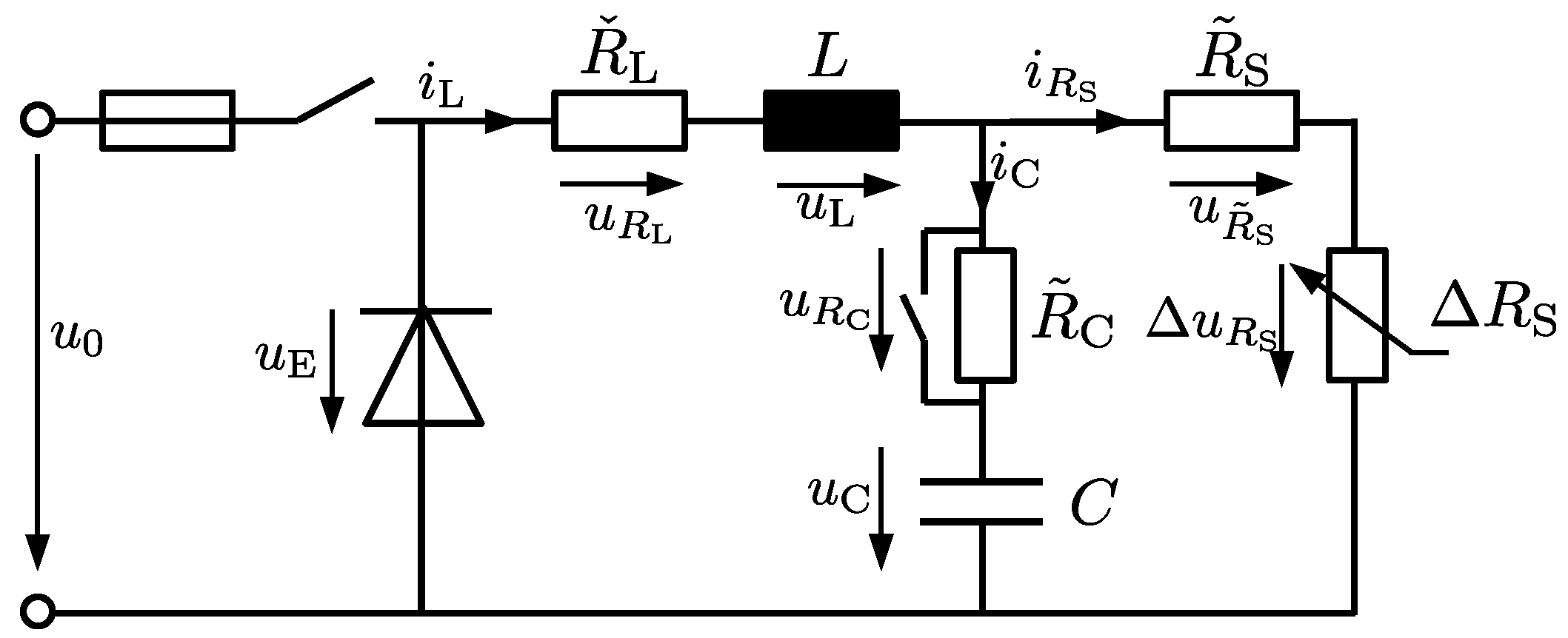
4. Application Scenario: Step-Down Converter
4.1. Modeling
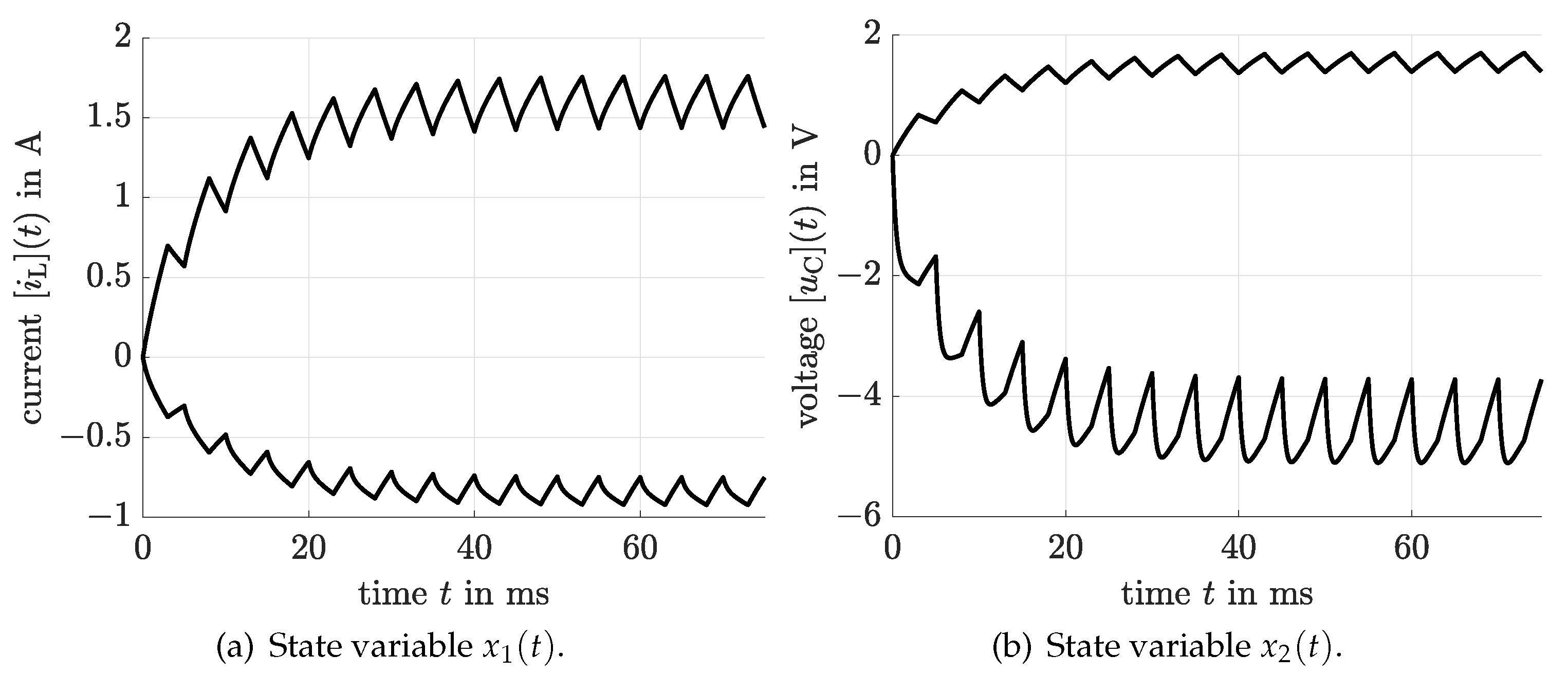
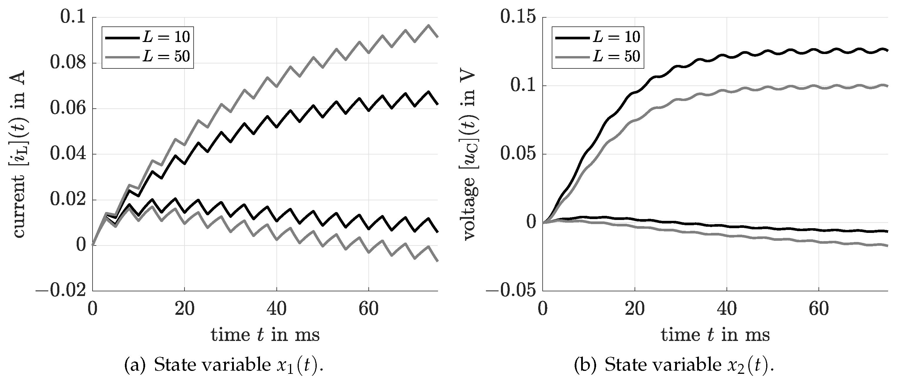
4.2. Simulation-Based Comparison of Two Cooperativity-Enforcing Similarity Transformations
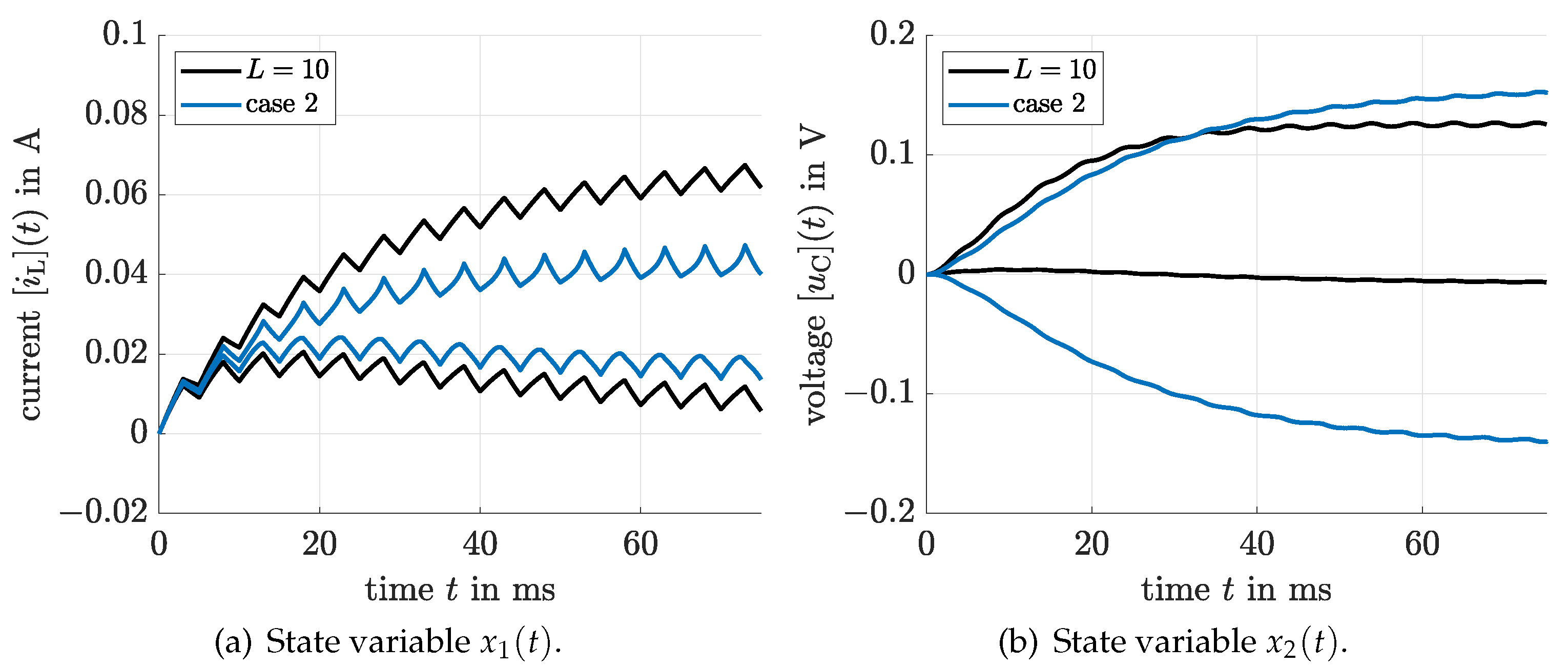
4.3. Comparison with a Taylor Model-Based Solution Approach
- case 1
- with default settings (order 12) for all options [43] except for the step size parameters and the choice of a QR preconditioningverifyodeset(’h0’, 1e-4, ’h_min’, 1e-6, ’precondition’, 1);
- case 2
- with order 10, manually specified small tolerances, and QR preconditioningverifyodeset(’order’, 10, ’shrinkwrap’, 0, ’precondition’, 1, ’blunting’, 0, ...’h0’, 1e-4, ’h_min’, 1e-6, ’loc_err_tol’, 1e-11, ’sparsity_tol’, 1e-20);
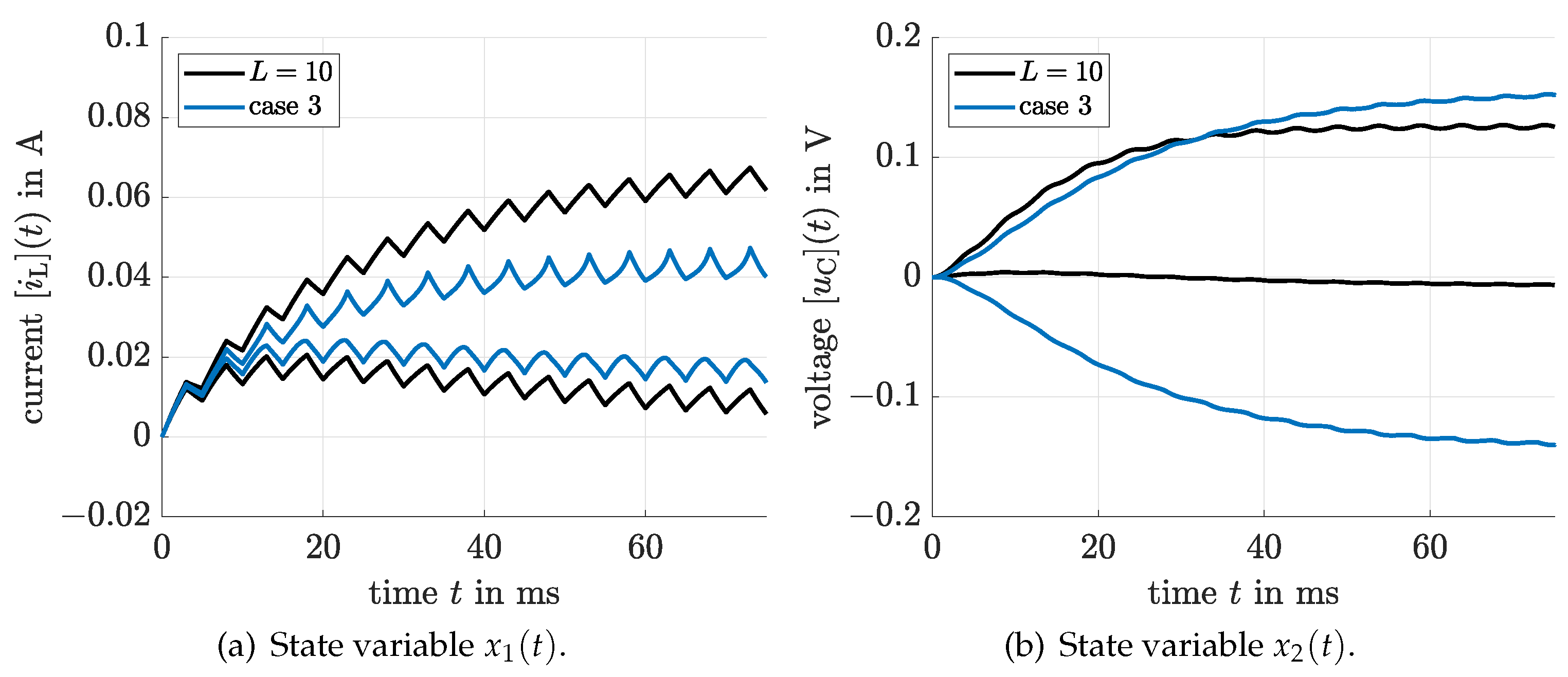
- case 3
- with order 30, manually specified small tolerances, and QR preconditioningverifyodeset(’order’, 30, ’shrinkwrap’, 0, ’precondition’, 1, ’blunting’, 0, ...’h0’, 1e-4, ’h_min’, 1e-6, ’loc_err_tol’, 1e-11, ’sparsity_tol’, 1e-20);
- case 4
- with order 10, manually specified small tolerances, and curvilinear preconditioningverifyodeset(’order’, 10, ’shrinkwrap’, 0, ’precondition’, 3, ’blunting’, 0, ...’h0’, 1e-4, ’h_min’, 1e-6, ’loc_err_tol’, 1e-11, ’sparsity_tol’, 1e-20);
- case 5
- with order 30, manually specified small tolerances, and curvilinear preconditioningverifyodeset(’order’, 30, ’shrinkwrap’, 0, ’precondition’, 3, ’blunting’, 0, ...’h0’, 1e-4, ’h_min’, 1e-6, ’loc_err_tol’, 1e-11, ’sparsity_tol’, 1e-20);
5. Conclusions and Future Work
Author Contributions
Funding
Data Availability Statement
Conflicts of Interest
References
- Raïssi, T.; Efimov, D.; Zolghadri, A. Interval State Estimation for a Class of Nonlinear Systems. IEEE Trans. Autom. Control 2012, 57, 260–265. [Google Scholar] [CrossRef]
- Efimov, D.; Raïssi, T.; Chebotarev, S.; Zolghadri, A. Interval State Observer for Nonlinear Time Varying Systems. Automatica 2013, 49, 200–205. [Google Scholar] [CrossRef]
- Mazenc, F.; Bernard, O. Asymptotically Stable Interval Observers for Planar Systems With Complex Poles. IEEE Trans. Autom. Control 2010, 55, 523–527. [Google Scholar] [CrossRef]
- Angeli, D.; Sontag, E. Monotone Control Systems. IEEE Trans. Autom. Control 2003, 48, 1684–1698. [Google Scholar] [CrossRef]
- Smith, H.L. Monotone Dynamical Systems: An Introduction to the Theory of Competitive and Cooperative Systems; Mathematical Surveys and Monographs, American Mathematical Soc.: Providence, RI, USA, 1995; Volume 41. [Google Scholar]
- Hirsch, M. On the Nonchaotic Nature of Monotone Dynamical Systems. Eur. J. Pure Appl. Math. 2019, 12, 680–688. [Google Scholar] [CrossRef]
- Rauh, A.; Kersten, J.; Aschemann, H. Interval and Linear Matrix Inequality Techniques for Reliable Control of Linear Continuous-Time Cooperative Systems with Applications to Heat Transfer. Int. J. Control 2020, 93, 2771–2788. [Google Scholar] [CrossRef]
- Raïssi, T.; Efimov, D. Some Recent Results on the Design and Implementation of Interval Observers for Uncertain Systems. at-Automatisierungstechnik 2018, 66, 213–224. [Google Scholar] [CrossRef]
- Nedialkov, N.S. Interval Tools for ODEs and DAEs. In Proceedings of the 12th GAMM-IMACS Intl. Symposium on Scientific Computing, Computer Arithmetic, and Validated Numerics SCAN 2006, Duisburg, Germany, 26–29 September 2006; IEEE Computer Society: Duisburg, Germany, 2007. [Google Scholar]
- Lohner, R. On the Ubiquity of the Wrapping Effect in the Computation of the Error Bounds. In Perspectives on Enclosure Methods; Kulisch, U., Lohner, R., Facius, A., Eds.; Springer–Verlag: Wien, NY, USA, 2001; pp. 201–217. [Google Scholar]
- Lohner, R. Enclosing the Solutions of Ordinary Initial and Boundary Value Problems. In Computer Arithmetic: Scientific Computation and Programming Languages; Kaucher, E.W., Kulisch, U.W., Ullrich, C., Eds.; Wiley-Teubner Series in Computer Science: Stuttgart, Germany, 1987; pp. 255–286. [Google Scholar]
- Kapela, T.; Mrozek, M.; Wilczak, D.; Zgliczynski, P. CAPD::DynSys: A Flexible C++ Toolbox for Rigorous Numerical Analysis of Dynamical Systems. Commun. Nonlinear Sci. Numer. Simul. 2020, 105578. [Google Scholar] [CrossRef]
- Berz, M.; Makino, K. COSY INFINITY Version 8.1. User’s Guide and Reference Manual; Technical Report MSU HEP 20704; Michigan State University: East Lansing, MI, USA, 2002. [Google Scholar]
- Hoefkens, J. Rigorous Numerical Analysis with High-Order Taylor Models. Ph.D. Thesis, Michigan State University, East Lansing, MI, USA, 2001. Available online: http://www.bt.pa.msu.edu/cgi-bin/display.pl?name=hoefkensphd (accessed on 14 January 2021).
- Alexandre dit Sandretto, J.; Chapoutot, A. Validated Explicit and Implicit Runge–Kutta Methods. Reliab. Comput. 2016, 22, 79–103. [Google Scholar]
- Mullier, O.; Chapoutot, A.; Alexandre dit Sandretto, J. Validated Computation of the Local Truncation Error of Runge–Kutta Methods with Automatic Differentiation. Optim. Methods Softw. 2018, 33, 718–728. [Google Scholar] [CrossRef]
- Rauh, A.; Auer, E.; Hofer, E.P. ValEncIA-IVP: A Comparison with Other Initial Value Problem Solvers. In Proceedings of the 12th GAMM-IMACS International Symposium on Scientific Computing, Computer Arithmetic, and Validated Numerics SCAN 2006, Duisburg, Germany, 26–29 September 2006; IEEE Computer Society: Duisburg, Germany, 2007. [Google Scholar]
- Auer, E.; Rauh, A.; Hofer, E.P.; Luther, W. Validated Modeling of Mechanical Systems with SmartMOBILE: Improvement of Performance by ValEncIA-IVP. In Proceedings of the Dagstuhl Seminar 06021: Reliable Implementation of Real Number Algorithms: Theory and Practice; Lecture Notes in Computer Science; Springer–Verlag: Berlin, Heidelberg, Germany, 2008; pp. 1–27. [Google Scholar]
- Rauh, A.; Westphal, R.; Aschemann, H.; Auer, E. Exponential Enclosure Techniques for Initial Value Problems with Multiple Conjugate Complex Eigenvalues. In Proceedings of 16th GAMM-IMACS International Symposium on Scientific Computing, Computer Arithmetic, and Validated Numerics SCAN2014; Lecture Notes in Computer Science; Springer: Cham, Switzerland, 2016; Volume 9553, pp. 87–122. [Google Scholar]
- Rauh, A.; Westphal, R.; Auer, E.; Aschemann, H. Exponential Enclosure Techniques for the Computation of Guaranteed State Enclosures in ValEncIA-IVP. 2013. Available online: http://interval.louisiana.edu/reliable-computing-journal/volume-19/reliable-computing-19-pp-066-090.pdf (accessed on 13 January 2021).
- Rauh, A.; Westphal, R.; Aschemann, H. Verified Simulation of Control Systems with Interval Parameters Using an Exponential State Enclosure Technique. In Proceedings of the IEEE 2013 18th International Conference on Methods and Models in Automation and Robotics MMAR, Miedzyzdroje, Poland, 26–29 August 2013. [Google Scholar]
- Nedialkov, N.S. Computing Rigorous Bounds on the Solution of an Initial Value Problem for an Ordinary Differential Equation. Ph.D. Thesis, Graduate Department of Computer Science, University of Toronto, Toronto, ON, Canada, 1999. [Google Scholar]
- Nedialkov, N.S. Implementing a Rigorous ODE Solver through Literate Programming. In Modeling, Design, and Simulation of Systems with Uncertainties; Rauh, A., Auer, E., Eds.; Mathematical Engineering, Springer: Berlin/Heidenberg, Germany, 2011; pp. 3–19. [Google Scholar]
- Lin, Y.; Stadtherr, M.A. Validated Solutions of Initial Value Problems for Parametric ODEs. Appl. Numer. Math. 2007, 57, 1145–1162. [Google Scholar] [CrossRef]
- Kaczorek, T. Positive 1D and 2D Systems; Springer–Verlag: London, UK, 2002. [Google Scholar]
- Gennat, M.; Tibken, B. Computing Guaranteed Bounds for Uncertain Cooperative and Monotone Nonlinear Systems. IFAC Proc. Vol. 2008, 41, 4846–4851. [Google Scholar] [CrossRef]
- Aschemann, H.; Rauh, A.; Kletting, M.; Hofer, E.; Gennat, M.; Tibken, B. Interval Analysis and Nonlinear Control of Wastewater Plants with Parameter Uncertainty. IFAC Proc. Vol. 2005, 38, 55–60. [Google Scholar] [CrossRef]
- Rauh, A.; Kersten, J.; Aschemann, H. Techniques for Verified Reachability Analysis of Quasi-Linear Continuous-Time Systems. In Proceedings of the 24th International Conference on Methods and Models in Automation and Robotics 2019, Miedzyzdroje, Poland, 26–29 August 2019. [Google Scholar]
- Kersten, J.; Rauh, A.; Aschemann, H. State-Space Transformations of Uncertain Systems With Purely Real and Conjugate-Complex Eigenvalues Into a Cooperative Form. In Proceedings of the 23rd International Conference on Methods and Models in Automation and Robotics 2018, Miedzyzdroje, Poland, 27–30 August 2018. [Google Scholar]
- Jaulin, L.; Kieffer, M.; Didrit, O.; Walter, É. Applied Interval Analysis; Springer–Verlag: London, UK, 2001. [Google Scholar]
- Mayer, G. Interval Analysis and Automatic Result Verification; De Gruyter Studies in Mathematics, De Gruyter: Berlin, Germany; Boston, MA, USA, 2017. [Google Scholar]
- Kühn, W. Rigorous Error Bounds for the Initial Value Problem Based on Defect Estimation; Technical Report. 1999. Available online: http://www.decatur.de/personal/papers/defect.zip (accessed on 13 January 2021).
- Kersten, J.; Rauh, A.; Aschemann, H. Interval Methods for Robust Gain Scheduling Controllers: An LMI-Based Approach. Granul. Comput. 2020, 5, 203–216. [Google Scholar] [CrossRef]
- Bünger, F. A Taylor Model Toolbox for Solving ODEs Implemented in MATLAB/INTLAB. J. Comput. Appl. Math. 2020, 368, 112511. [Google Scholar] [CrossRef]
- Müller, M. Über die Eindeutigkeit der Integrale eines Systems gewöhnlicher Differenzialgleichungen und die Konvergenz einer Gattung von Verfahren zur Approximation dieser Integrale; Sitzungsbericht Heidelberger Akademie der Wissenschaften; Walter de Gruyter GmbH & Co KG: Berlin, Germany, 1927. [Google Scholar]
- Rauh, A.; Kersten, J.; Aschemann, H. Interval Methods and Contractor-Based Branch-and-Bound Procedures for Verified Parameter Identification of Quasi-Linear Cooperative System Models. J. Comput. Appl. Math. 2020, 367, 112484. [Google Scholar] [CrossRef]
- Boyd, S.; El Ghaoui, L.; Feron, E.; Balakrishnan, V. Linear Matrix Inequalities in System and Control Theory; SIAM: Philadelphia, PA, USA, 1994. [Google Scholar]
- Sturm, J. Using SeDuMi 1.02, A MATLAB Toolbox for Optimization over Symmetric Cones. Optim. Methods Softw. 1999, 11–12, 625–653. [Google Scholar] [CrossRef]
- Löfberg, J. YALMIP: A Toolbox for Modeling and Optimization in MATLAB. In Proceedings of the IEEE International Symposium on Computer Aided Control Systems Design, Taipei, Taiwan, 2–4 September 2004; pp. 284–289. [Google Scholar]
- Rump, S. IntLab—INTerval LABoratory. In Developments in Reliable Computing; Csendes, T., Ed.; Kluver Academic Publishers: Dordrecht, The Netherlands, 1999; pp. 77–104. [Google Scholar]
- Freihold, M.; Hofer, E. Derivation of Physically Motivated Constraints for Efficient Interval Simulations Applied to the Analysis of Uncertain Dynamical Systems. Appl. Math. Comput. Sci. 2009, 19, 485–499. [Google Scholar] [CrossRef]
- Freihold, M.; Rauh, A.; Hofer, E.P. Physically Motivated Constraints for Efficient Interval Simulations Applied to the Analysis of Uncertain Models of Blood Cell Dynamics. In Progress in Industrial Mathematics at ECMI 2008; Fitt, A.D., Norbury, J., Ockendon, H., Wilson, E., Eds.; Springer: Berlin/Heidelberg, Germany, 2010; pp. 563–569. [Google Scholar]
- Bünger, F. DEMOTAYLORMODEL Short Demonstration of the Taylor Model Toolbox. Available online: www.ti3.tuhh.de/intlab/demos/html/dtaylormodel.html (accessed on 16 February 2021).
- Bünger, F. Preconditioning of Taylor Models, Implementation and Test Cases. Nonlinear Theory Its Appl. IEICE 2021, 12, 2–40. [Google Scholar] [CrossRef]
- Bünger, F. Shrink Wrapping for Taylor Models Revisited. Numer. Algorithms 2018, 78, 1001–1017. [Google Scholar] [CrossRef]
- Rauh, A.; Kersten, J. Toward the Development of Iteration Procedures for the Interval-Based Simulation of Fractional-Order Systems. Acta Cybern. 2020. [Google Scholar] [CrossRef]
- Rauh, A.; Kersten, J. Verification and Reachability Analysis of Fractional-Order Differential Equations Using Interval Analysis. In Proceedings 6th International Workshop on Symbolic-Numeric Methods for Reasoning about CPS and IoT, Online, 31 August 2020; Electronic Proceedings in Theoretical Computer Science; Dang, T., Ratschan, S., Eds.; Open Publishing Association: Den Haag, The Netherlands, 2021; Volume 331, pp. 18–32. [Google Scholar] [CrossRef]
- Rauh, A.; Jaulin, L. Novel Techniques for a Verified Simulation of Fractional-Order Differential Equations. Fractal Fract. 2021, 5, 17. [Google Scholar] [CrossRef]


Publisher’s Note: MDPI stays neutral with regard to jurisdictional claims in published maps and institutional affiliations. |
© 2021 by the authors. Licensee MDPI, Basel, Switzerland. This article is an open access article distributed under the terms and conditions of the Creative Commons Attribution (CC BY) license (http://creativecommons.org/licenses/by/4.0/).
Share and Cite
Rauh, A.; Kersten, J. Transformation of Uncertain Linear Systems with Real Eigenvalues into Cooperative Form: The Case of Constant and Time-Varying Bounded Parameters. Algorithms 2021, 14, 85. https://doi.org/10.3390/a14030085
Rauh A, Kersten J. Transformation of Uncertain Linear Systems with Real Eigenvalues into Cooperative Form: The Case of Constant and Time-Varying Bounded Parameters. Algorithms. 2021; 14(3):85. https://doi.org/10.3390/a14030085
Chicago/Turabian StyleRauh, Andreas, and Julia Kersten. 2021. "Transformation of Uncertain Linear Systems with Real Eigenvalues into Cooperative Form: The Case of Constant and Time-Varying Bounded Parameters" Algorithms 14, no. 3: 85. https://doi.org/10.3390/a14030085
APA StyleRauh, A., & Kersten, J. (2021). Transformation of Uncertain Linear Systems with Real Eigenvalues into Cooperative Form: The Case of Constant and Time-Varying Bounded Parameters. Algorithms, 14(3), 85. https://doi.org/10.3390/a14030085