Constant-Time Complete Visibility for Robots with Lights: The Asynchronous Case ^†

Abstract

We consider the distributed setting of N autonomous mobile robots that operate in Look-Compute-Move (LCM) cycles and use colored lights (the robots with lights model). We assume obstructed visibility where a robot cannot see another robot if a third robot is positioned between them on the straight line segment connecting them. In this paper, we consider the problem of positioning N autonomous robots on a plane so that every robot is visible to all others (this is called the Complete Visibility problem). This problem is fundamental, as it provides a basis to solve many other problems under obstructed visibility. In this paper, we provide the first, asymptotically optimal, $\mathcal{O}\left(1\right)$ time, $\mathcal{O}\left(1\right)$ color algorithm for Complete Visibility in the asynchronous setting. This significantly improves on an $\mathcal{O}\left(N\right)$-time translation of the existing $\mathcal{O}\left(1\right)$ time, $\mathcal{O}\left(1\right)$ color semi-synchronous algorithm to the asynchronous setting. The proposed algorithm is collision-free, i.e., robots do not share positions, and their paths do not cross. We also introduce a new technique for moving robots in an asynchronous setting that may be of independent interest, called Beacon-Directed Curve Positioning.

1. Introduction

The classical model of distributed computing by mobile robots models each robot as a point in the plane that is equipped with a local coordinate system and sensory capabilities to determine the positions of other robots [1]. The local coordinate system of a robot may not be consistent with that of other robots. The sensory capability of a robot, generally called vision, allows a robot to determine the positions of other robots in its own coordinate system. The robots are autonomous (no external control), anonymous (no unique identifiers), indistinguishable (no external identifiers), and disoriented (no agreement on local coordinate systems or units of distance measures).

They execute the same algorithm. Typically, robots have unobstructed visibility, that is, robots are transparent such that three collinear robots can see each other. Each robot proceeds in Look-Compute-Move (LCM) cycles: When a robot becomes active, it first gets a snapshot of its surroundings (Look), then computes a destination based on the snapshot (Compute), and finally moves towards the destination (Move). Moreover, the robots are oblivious, i.e., in each cycle, each robot has no memory of its past LCM cycles [1]. Furthermore, the robots are silent because they do not communicate directly, and only vision and mobility enable them to coordinate their actions.

While silence has advantages, many other situations, e.g., hostile environments, assume direct communication. The robots with lights model [1,2,3] incorporates direct communication, where each robot has an externally visible light that can assume colors from a constant-sized set; robots explicitly communicate with each other using these colors. The colors are persistent, i.e., the color is not erased at the end of a cycle. Except for the lights, the robots are oblivious as in the classical model. In addition, robots have obstructed visibility such that robot b in line between robots a and c blocks the views of a from c and vice versa.

The following fundamental problem, Complete Visibility on the robots with lights model is the main focus of this paper. Given an arbitrary initial configuration of N robots located at distinct points on a real plane, they autonomously arrange themselves in a configuration in which each robot is in a distinct position and from which it can see all other robots. In the initial configuration, some robots may be obstructed from the view of others and the robots themselves do not know the total number of robots, N. Solving Complete Visibility enables solutions to many other robot problems under obstructed visibility, including gathering, pattern formation, and leader election. For example, we recently solved the problem of pattern formation in Reference [4], which uses the solution to Complete Visibility presented in this paper in the first step of its four-step algorithm. Indeed, after the robots reach a configuration of complete visibility, they know the value of N and each robot can see all the robots in the system as in robots model with unobstructed visibility, i.e., any solution to Complete Visibility recovers unobstructed visibility configuration starting from an obstructed visibility configuration.

Di Luna et al. [5] gave the first algorithm for robots with lights to solve Complete Visibility on a real plane. They arranged robots on the corners of a N-corner convex hull, which immediately solves Complete Visibility since each robot positioned on a corner of a convex hull sees all other $N-1$ robots positioned on $N-1$ other corners. In the real-world setting, the convex hull based Complete Visibility solution might also help to make a barrier around the site of interest so that the intruders entering the site from one point may be monitored and reported to all the points of interests (provided by robots). Di Luna et al. [5] focused mostly on correctness proving that the problem can be solved in finite time. The question of minimizing the number of colors and the precise bound on runtime was left open. References [6,7] provided solutions minimizing number of colors with finite runtime. References [8,9] provided solutions with provable runtime bounds keeping the number of colors constant. For example, Reference [9] showed that Complete Visibility can be solved in $\mathcal{O}\left(1\right)$ time using $\mathcal{O}\left(1\right)$ colors in the semi-synchronous setting. There is no existing work that provides a runtime bound for Complete Visibility in the asynchronous setting, which is the main goal of this paper.

A straightforward algorithm can be designed to solve Complete Visibility in the asynchronous setting with runtime $\mathcal{O}\left(N\right)$ using $\mathcal{O}\left(1\right)$ colors, combining the semi-synchronous algorithm of Reference [9] for Complete Visibility with the result of Das et al. [2]. The result of Das et al. [2] is as follows: Any algorithm (for any problem) in the robots with lights model that uses $k>1$ colors in the semi-synchronous setting can be simulated in the asynchronous setting with, at most, $5·k$ colors. Since the semi-synchronous Complete Visibility algorithm of Reference [9] uses 12 colors, the total number of colors in the new algorithm becomes $5·12=60=\mathcal{O}\left(1\right)$. However, Das et al. [2] does not say anything about the runtime of their simulation and it can be shown that, for N robots, this combination increases the runtime by a $\mathcal{O}\left(N\right)$-factor, meaning that $\mathcal{O}\left(1\right)$ runtime for Complete Visibility in the semi-synchronous setting becomes $\mathcal{O}\left(N\right)$ time for Complete Visibility in the asynchronous setting. In this paper, we present an algorithm for Complete Visibility that runs in $\mathcal{O}\left(1\right)$ time using $\mathcal{O}\left(1\right)$ colors even in the asynchronous setting. Note that $\mathcal{O}\left(1\right)$ runtime is optimal for Complete Visibility, irrespective of the number of colors.

1.1. Contributions

The robot model used in this paper is the same one as in Di Luna et al. [5]; namely, robots are oblivious except for a persistent light that can assume a constant number of colors. The robots considered here are points. If robots have mass and occupy an area (and volume), then the algorithm we present will not work, and a different algorithm needs to be designed that works respecting the mass of the robots. There is a line of work that solves Complete Visibility for the robots with mass; please refer to References [10,11,12] for some of the most recent works in that line of work. Robots’ visibility can be obstructed by other robots in the line of sight, robots are unaware of the number, N, of robots in the swarm, and the robots may be disoriented. Further, we assume that the robot setting is asynchronous, i.e., there is no notion of common time and robots perform their Look-Compute-Move cycles at arbitrary time. Robot moves robots are rigid, i.e., a robot in motion cannot be stopped (by an adversary) before it reaches its destination point. Our algorithms are collision-free; that is, two robots do not head to the same destination, and their paths of motion do not cross.

In Section 3, we develop a framework called Beacon-Directed Curve Positioning that moves a set of robots onto a (k-point) curve in $\mathcal{O}(logk)$ time using three colors in the asynchronous setting, under the condition that $2k$ robots (called beacons) are already properly laid out on the curve. Furthermore, robots move need to be collision-free, and their paths cannot intersect the curve at more than one point (Definition 2).

Using this framework, we prove the following result (comparison is in Table 1), which, to our knowledge, is the first algorithm for Complete Visibility that achieves sub-linear runtime for robots with lights in the asynchronous setting. In fact, this runtime is asymptotically optimal as $\mathsf{\Omega }\left(1\right)$ is a trivial lower bound for the problem.

Table 1. Comparison of Complete Visibility results for the robots with lights model with monotonic movements on a 2-dimensional Euclidean plane.

Source	Model	Runtime	No. of Colors
Di Luna et al. [5], Di Luna et al. [6], Sharma et al. [7]	asynchronous	–	10, 3, 2 $=\mathcal{O}\left(1\right)$
Vaidyanathan et al. [8]	fully synchronous	$\mathcal{O}(logN)$	12 $=\mathcal{O}\left(1\right)$
Sharma et al. [9]	semi-synchronous	$\mathcal{O}\left(1\right)$	12 $=\mathcal{O}\left(1\right)$
Das et al. [2] with Sharma et al. [9]	asynchronous	$\mathcal{O}\left(N\right)$	60 $=\mathcal{O}\left(1\right)$
Theorem 1	asynchronous	$\mathcal{O}\left(1\right)$	47 $=\mathcal{O}\left(1\right)$

Theorem 1.

For any initial configuration of $N\ge 1$ robots with lights in distinct positions on a real plane, there is an algorithm that solvesComplete Visibilityin the asynchronous setting in $\mathcal{O}\left(1\right)$ time with $\mathcal{O}\left(1\right)$ colors and without collisions.

Our algorithm is deterministic and has three stages, Stages 0–2, that execute one after another. Stage 0 is needed only if the initial configuration has robots on a straight line; it breaks this initial linear arrangement and places all robots within or on a convex polygon $\mathbf{P}$ (convex hull of points) in $\mathcal{O}\left(1\right)$ time. After that, Stage 1 places all robots on the corners and sides of a convex polygon ${\mathbf{P}}^{″}$. ($\mathbf{P}$ is first transformed to ${\mathbf{P}}^{\prime }$, which is completely contained inside $\mathbf{P}$, and then ${\mathbf{P}}^{\prime }$ is transformed to ${\mathbf{P}}^{″}$. All this happens during Stage 1, which operates in five sub-stages, Stage 1.1–1.5.) Finally, Stage 2 moves each robot on a side of polygon ${\mathbf{P}}^{″}$ to a corner of a new convex polygon ${\mathbf{P}}^{‴}$ (the points that are positioned on the corners of ${\mathbf{P}}^{″}$ do not move at this stage). (The precise definitions of all these convex polygons are given later in Section 2). Keys to Stage 1 are corner moving, internal moving, and the beacon-directed curve positioning procedures that permit all interior robots of $\mathbf{P}$ to move to the sides of ${\mathbf{P}}^{″}$ executing each stage in $\mathcal{O}\left(1\right)$ time, even in the asynchronous setting. An important part of Stage 2 is a corner insertion procedure that moves side robots of ${\mathbf{P}}^{″}$ to corners of ${\mathbf{P}}^{‴}$ in $\mathcal{O}\left(1\right)$ time while retaining convexity.

This paper is a combination of the ideas presented in IPDPS’17 [13] and SSS’17 [14]. We proved all the properties of Theorem 1 in Reference [13] (IPDPS’17), except that the runtime is $\mathcal{O}(logN)$. Moreover, there were three stages, Stages 0–2, with Stage 1 having 5 sub-stages, Stage 1.1–1.5. Stages 0 and 2 run in $\mathcal{O}\left(1\right)$ time, and Stages 1.1 and 1.4 also run in $\mathcal{O}\left(1\right)$ time. The $\mathcal{O}(logN)$ time was due to the run time of Stages 1.2, 1.3, and 1.5, each of them taking $\mathcal{O}(logN)$ time. The Beacon-Directed Curve Positioning framework developed in Reference [14] (SSS’17) allows to run Stages 1.2, 1.3, and 1.5 in $\mathcal{O}\left(1\right)$ time each, giving overall time complexity $O\left(1\right)$. Therefore, the combination of the ideas of [13,14] makes the runtime of $O\left(1\right)$ claimed in this paper possible.

1.2. Related Work

The problem of Complete Visibility has been getting much attention recently, after it was proposed for the very first time by Di Luna et al. [5] in 2014. They proposed the problem on a 2-dimesional real plane and we also consider the problem on the real plane. The most closely related works on a plane are listed in Table 1. Di Luna et al. [5] designed the first algorithm for robots with lights to solve Complete Visibility. Their algorithm uses 6 colors in the semi-synchronous setting and 10 colors in the asynchronous setting. Their algorithm arranged robots on corners of a convex polygon, which naturally solves this problem. Although other ways exist to solve Complete Visibility without forming a convex hull, such a convex hull solution provides additional advantages [10,15] in solving some other problems. One example is our recent work on pattern formation [4], where we use the convex hull based Complete Visibility result of this paper in the first step of the four-step algorithm for pattern formation in the asynchronous setting presented in that paper. In this paper, we, too, form a convex hull as a solution to Complete Visibility. Di Luna et al. [5] established the correctness of their algorithm, including a proof of (finite-time) termination; however, the work does not include a runtime analysis. Subsequent work [6,7] reduced the number of colors used for the algorithm. The minimum number of colors is 2, and Sharma et al. provided 2-color algorithm for the semi-synchronous and asynchronous settings of monotonic robot movements (defined later) and 3-color algorithm in the asynchronous setting with non-monotonic robot movements. Therefore, with respect to optimizing the number of colors, there is not much work left except designing a 2-color algorithm for the asynchronous setting of non-monotonic robot movements.

Therefore, the recent focus is mostly on runtime [8,9], keeping the number of colors constant, i.e., $\mathcal{O}\left(1\right)$. Runtime is a critical factor when robots have to arrange themselves in a target configuration, frequently while working in real-time after being deployed in their work environments. In this direction, Vaidyanathan et al. [8] designed the first algorithm with $\mathcal{O}(logN)$ runtime, and with the use of $\mathcal{O}\left(1\right)$ colors in the fully synchronous setting. Sharma et al. [9] improved on this result with $\mathcal{O}\left(1\right)$ runtime using $\mathcal{O}\left(1\right)$ colors in the semi-synchronous setting. Whether this $\mathcal{O}\left(1\right)$ runtime, $\mathcal{O}\left(1\right)$ colors result extends to the asynchronous setting, is an important open question left from these existing works, which we address in this paper by designing such an algorithm that works in $\mathcal{O}\left(1\right)$ time using $\mathcal{O}\left(1\right)$ colors. Of the three models typically considered, fully synchronous, semi-synchronous, and asynchronous, the asynchronous setting is the weakest, and full synchronous is the strongest; asynchronous algorithms present significant challenges in their design and analysis. Therefore, our work considers the problem in the most difficult setting, and, since the algorithm we present works in this most difficult setting, it subsumes all the existing works designed for the relatively simpler fully synchronous and semi-synchronous settings.

It is interesting to consider whether Complete Visibility can be solved when robots may experience faults. Di Luna et al. [6] observed that their Complete Visibility algorithm for non-faulty robots can solve Complete Visibility tolerating a faulty robot if the faulty robot is in the perimeter of the convex hull formed by the initial configuration of the robots. Aljohani and Sharma [16] provided an algorithm that tolerates one faulty robot (irrespective of whether the faulty robot is in the interior or not) when robots have both-axis agreement in the semi-synchronous setting under rigid movements. The idea was to position all the robots on the corners of a convex hull except the faulty robot that may still be in the interior of the hull in the final configuration. Aljohani and Sharma [16] also showed that Complete Visibility can be solved tolerating, at most, 2 faulty robots under certain assumptions on initial configurations. Recently, Poudel et al. [17] assumed a weaker one-axis agreement and presented an algorithm for Complete Visibility in the asynchronous setting that can tolerate any number of faulty robots. An interesting property of their algorithm is that it solves Complete Visibility without arranging (non-faulty) robots on the corners of a convex hull.

Complete Visibility was also studied in the classical oblivious robots model (no lights) [1]. Di Luna et al. [15] provided the first algorithm in this model considering the semi-synchronous setting. Sharma et al. [12] then provided an algorithm with runtime $\mathcal{O}\left(N\right)$ in this model under the fully synchronous setting. They also showed that the algorithm of Di Luna et al. [15] has runtime $\mathsf{\Omega }\left(N^2\right)$. Bhagat et al. [18] solved Complete Visibility under one-axis agreement in the asynchronous setting.

Recently, Complete Visibility was also studied in the so-called fat robots model (with or without lights) [10,19] in which robots are not points, but non-transparent unit discs with mass occupiying certain area. In the fat robots with lights model, Sharma et al. [11] provided an $\mathcal{O}\left(N\right)$ runtime Complete Visibility algorithm using 9 colors in the fully synchronous setting under rigid (monotonic) movements. In the fat robots (without lights) model, Sharma et al. [12] provided an $\mathcal{O}\left(N\right)$ runtime Complete Visibility algorithm in the semi-synchronous setting under rigid movements, with some assumptions on the initial configurations.

Additionally, there is a recent interest in solving Complete Visibility in the grid setting, which discretizes the Euclidean real plane. The grid setting is interesting from the aspect of real applications of robots. Adhikary et al. [20] provided a solution to Complete Visibility using 11 colors in the grid setting and no runtime analysis. We provided an algorithm with a provable runtime bound keeping the number of colors constant [21]. These solutions do not arrange robots on the corners of a convex hull, in contrast to what we do in this paper. Finally, Hector et al. [22] provided matching lower and upper bounds on arranging robots on a convex hull in the grid setting, analogous to what we do in this paper.

Beyond Complete Visibility, the computational power of the robots with lights compared to classical oblivious robots was studied in Reference [2], while the robots are working on the Euclidean plane, and in Reference [23], while the robots are working on graphs.

The obstructed visibility, in general, was also considered in the different problems in different settings. One problem that considers obstructed visibility is the problem of uniform spreading of robots on a line [24]. The robots considered there are classical robots [1] (without lights). The fat robots model, in which an individual robot is a unit disc (rather than a point), also assumes obstructed visibility [10,19,25,26,27]. However, this body of work do not analyze runtime. Pagli et al. [28] study the problem of collision-free Gathering classical robots to a small area; however, they do not provide a runtime analysis. Similarly, much work on the classical robot model [24,29,30,31] for Gathering does not have runtime analysis, except in a few cases [32,33,34,35,36]. Furthermore, Izumi et al. [37] considered the robot scattering problem (opposite of Gathering) in the semi-synchronous setting and provided a solution with an expected runtime of $\mathcal{O}(min\{N,D^2+logN\})$; here, D is the diameter of the initial configuration. Our paper focuses on runtime analysis and provides an optimal $\mathcal{O}\left(1\right)$ runtime algorithm for Complete Visibility on a plane for point robots in the lights model in the asynchronous setting keeping the number of colors constant. It will be interesting to see where our runtime approach can help to provide runtime bounds for some/all problems that we discussed above in the paragraph.

1.3. Roadmap

In Section 2, we detail the robot model and discuss some preliminaries. We define the beacon directed framework for positioning a set of robots on a curve in Section 3. Section 4, Section 5, Section 6 and Section 7 are devoted to proving Theorem 1 using the framework of Section 3. In Section 8, we provide some concluding remarks.

2. Model and Preliminaries

• Robots

Let $\mathcal{Q}=\{r_0,r_1,\cdots ,r_{N-1}\}$ be a set of N robots (agents) in a distributed system. Each robot is represented as a (dimensionless) point that moves in ${\mathbb{R}}^2$, the infinite 2-dimensional real plane. In this paper, a point will denote a robot, as well as its position. A robot $r_i$ can see, and be visible to, another robot $r_j$ iff there is no third robot $r_k$ in the line segment joining $r_i$ and $r_j$. Each robot has a light that can assume one color at a time; this color comes from a set with a constant number of colors.

• Look-Compute-Move

At any given time, a robot $r_i$ can be active or inactive. When robot $r_i$ becomes active, it performs the “Look-Compute-Move” (LCM) cycle described below.

• Look: For each robot $r_j$ that is visible to $r_i$, robot $r_i$ observes the position of $r_j$ and the color of its light. It is assumed that $r_i$ is visible to itself.
  Each robot observes position of other robots accurately, but within its own local frame of reference. That is, two different robots observing the position of the same point may produce different coordinates.
• Compute: After observing the position and light color of visible robots, robot $r_i$ may perform an arbitrary computation using only the positions and colors observed during the “look” portion of the current LCM cycle. This computation includes determination of a (possibly) new position to move to and light color for robot $r_i$ for the start of next cycle.
• Move: At the end of the LCM cycle, robot $r_i$ changes its light to the new color (determined during the compute phase) and moves to its new position.
  Robot $r_i$ maintains this new light color from the current LCM cycle until it is possibly changed in the move phase of the next LCM cycle.

• Robot Activation and Synchronization

In the fully synchronous setting ($\mathcal{FSYNC}$), every robot is active in every LCM cycle. In the semi-synchronous setting ($\mathcal{SSYNC}$), at least one robot is active, and over an infinite number of LCM cycles, every robot is active infinitely often. In the asynchronous setting ($\mathcal{ASYNC}$), robots have no common notion of time. No limit exists on the number and frequency of LCM cycles in which a robot can be active except that every robot is active infinitely often. Complying with the $\mathcal{ASYNC}$ setting, we assume that a robot “wakes up” and performs its Look phase at an instant of time. An arbitrary amount of time may elapse between the Look and Compute phases and between the Compute and Move phases. We also assume that during the Move phase it moves in a straight line at some (not necessarily constant) speed, but without stopping or changing direction. We will call such robot moves monotonic movements.

• Runtime

For the $\mathcal{FSYNC}$ setting, time is measured in rounds. Since a robot in the $\mathcal{SSYNC}$ and $\mathcal{ASYNC}$ settings could stay inactive for an indeterminate number of rounds, we introduce the idea of an epoch to measure runtime. An epoch is the smallest number of rounds within which each robot is active at least once [38]. Let $t_0$ denote the start time of the algorithm. Epoch i ($i\ge 1$) is the time interval from $t_{i-1}$ to $t_i$ where $t_i$ is the first time instance after $t_{i-1}$ when each robot has completed at least one complete LCM cycle. Therefore, for the $\mathcal{FSYNC}$ setting, a round is an epoch. We will use the term “time” generically to mean rounds for the $\mathcal{FSYNC}$ setting and epochs for the $\mathcal{SSYNC}$ and $\mathcal{ASYNC}$ settings.

• Convex Polygon

For $N\ge 3$, represent a convex polygon as a sequence $\mathbf{P}=(c_0,c_1,\cdots ,c_{N-1})$ of corner points in a plane that enumerates the polygon vertices in clockwise order. Figure 1 shows a 5-corner convex polygon $(c_0,c_1,c_2,c_3,c_4)$. A point s on the plane is a side point of $\mathbf{P}$ iff there exists $0\le i<N$ such that $c_i,s,c_{(i+1)\left(\mathrm{mod}N\right)}$ are collinear. Figure 1 shows nine side points $s_1$–$s_9$. A side $S=(c_i,s_1,s_2,\cdots ,s_m,c_{i+1})$ is a sequence of collinear points in which its beginning and end are adjacent corner points and in which its remaining points are side points. For any pair of points $a,b$, we denote the line segment connecting them by $\overline{ab}$ and the length of this segment by $\mathsf{length}\left(\overline{ab}\right)$. Moreover, we denote the infinite line passing through $a,b$ by $\overleftrightarrow{ab}$.

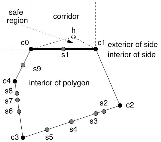
Figure 1. A convex polygon $\mathbf{P}=(c_0,c_1,c_2,c_3,c_4)$ with five corner points $c_i$ and nine side points $s_j$. The figure also illustrates the interior and exterior of side $\overline{c_0{c}_1}$.

A given polygon $\mathbf{P}$ divides the plane into interior and exterior parts. Figure 1 shows the interior of the polygon (the rest of the plane is the exterior). For a given side S of $\mathbf{P}$, the infinite line obtained by extending side S divides the plane into the interior and exterior parts of the side. The interior part of S contains the interior of the polygon. Figure 1 shows the interior and exterior of side $\overline{c_0{c}_1}$. The corridor of S is the infinite subregion on its exterior that is bounded by S and perpendicular lines through points $c_i,c_{i+1}$ of S. The corridors of the sides of $\mathbf{P}$ are disjoint except for the corner points.

• Configuration and Local Convex Polygon

A configuration ${\mathbf{C}}_t=\{(r_0^t,co{l}_0^t),\dots ,(r_{N-1}^t,co{l}_{N-1}^t)\}$ defines the positions of the robots in $\mathcal{Q}$ and their colors for any time $t\ge 0$. A configuration for a robot $r_i\in \mathcal{Q}$, ${\mathbf{C}}_t\left(r_i\right)$, defines the positions of the robots in $\mathcal{Q}$ that are visible to $r_i$ (including $r_i$) and their colors, i.e., ${\mathbf{C}}_t\left(r_i\right)\subseteq {\mathbf{C}}_t$, at time t. The convex polygon formed by ${\mathbf{C}}_t\left(r_i\right)$, ${\mathbf{P}}_t\left(r_i\right)$, is local to $r_i$ since ${\mathbf{P}}_t\left(r_i\right)$ depends on the points that are visible to $r_i$ at time t. We sometimes write $\mathbf{C},\mathbf{P},\mathbf{C}\left(r_i\right),\mathbf{P}\left(r_i\right)$ to denote ${\mathbf{C}}_t,{\mathbf{P}}_t,{\mathbf{C}}_t\left(r_i\right),{\mathbf{P}}_t\left(r_i\right)$, respectively.

• Corner Triangle, Corner Line Segment, Triangle Line Segment, and Corner Polygon

Let $c_i$ be a corner of a convex polygon $\mathbf{P}$. Let $c_{i-1}$ and $c_{i+1}$ be the neighboring corners of $c_i$ on the boundary of $\mathbf{P}$. Let $x_i,y_i$ be the points on sides $\overline{c_i{c}_{i-1}}$ and $\overline{c_i{c}_{i+1}}$ at distance $\mathsf{length}\left(\overline{c_i{c}_{i-1}}\right)/8$ and $\mathsf{length}\left(\overline{c_i{c}_{i+1}}\right)/8$, respectively, from $c_i$. We pick distance 1/8-th for our convenience; in fact, any factor less than or equal to $1/2$ works for our algorithm. We say that triangle $c_i{x}_i{y}_i$ is the corner triangle for $c_i$, denoted as $T\left(c_i\right)$, and line segment $\overline{x_i{y}_i}$ is the triangle line segment for $c_i$, denoted as $T{L}_i$. We say that the interior of $\mathbf{P}$ except the corner triangles is the special polygon of $\mathbf{P}$, denoted $\mathbf{S}\left(\mathbf{P}\right)$. Let r be any robot inside $T\left(c_i\right)$ and $S_i$ be the line segment parallel to $\overline{x_i{y}_i}$ passing through r. Let $T^{\prime }\left(r\right)$ be the portion of $T\left(c_i\right)$ between $S_i$ and $c_i$. We say that $S_i$ is the corner line segment for $c_i$, denoted as $C{L}_i$, if there is no robot inside $T^{\prime }\left(r\right)$. Let $L_{i-1},L_{i+1}$ be the lines perpendicular to $\overline{c_i{c}_{i-1}}$ and $\overline{c_i{c}_{i+1}}$, respectively, passing through their midpoints. We say the interior of $\mathbf{P}$ divided by $L_{i-1},L_{i+1}$ towards $c_i$ is the corner polygon of $c_i$, denoted as $CP\left(c_i\right)$. Figure 2 shows $T\left(c_i\right)$, $T{L}_3$, $C{L}_3$, $CP\left(c_3\right)$, and a 5-corner convex polygon $\mathbf{P}$ with corners $c_0-c_4$.

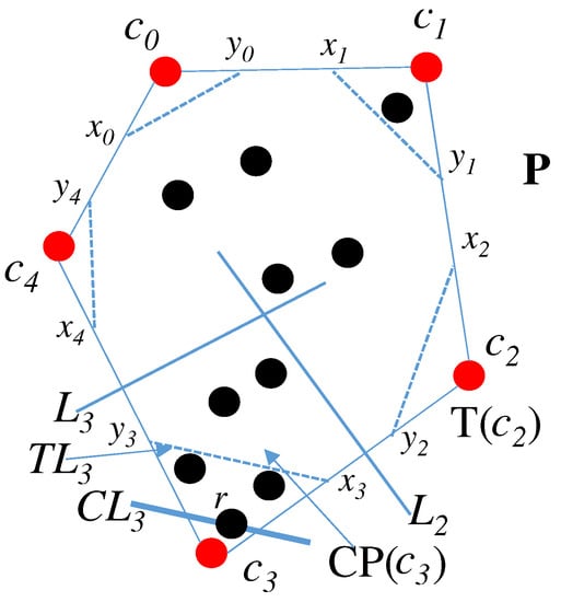
Figure 2. Example of corner triangle, corner line segment, triangle line segment, and corner polygon.

• Eligible Area and Eligible Line

Let $c_i$ be a corner of $\mathbf{P}$ and let $a,b$ be the neighbors (sides or corners) of $c_i$ in the perimeter of $\mathbf{P}$, and let u, w be the midpoints of $\overline{c_{i}a}$, $\overline{c_{i}b}$, respectively. The eligible area for $c_i$, denoted as $EA\left(c_i\right)$, is a polygonal subregion inside $\mathbf{P}$ within triangle $c_{i}uw$, omitting the lines from each robot to $c_i$ [9]. The eligible areas for any two corners of $\mathbf{P}$ are disjoint. $EA\left(c_i\right)$ is computed based on $\mathbf{C}\left(c_i\right)$ and the corresponding polygon $\mathbf{P}\left(c_i\right)$. Figure 3 depicts eligible area for $c_i$ where the shaded area is $EA\left(c_i\right)$. To make sure that all the robots in the interior of $\mathbf{P}$ see $c_i$ when it moves to a point in $EA\left(c_i\right)$, the points inside the outer boundary of $EA\left(c_i\right)$ that are part of the lines $\overleftrightarrow{c_{i}x}$, connecting $c_i$ with all the robots in $\mathbf{C}\left(c_i\right)\backslash \{a,b,c_i\}$ are not considered as the points of $EA\left(c_i\right)$. When $c_i$ moves to any point inside $EA\left(c_i\right)$, two prominent properties of the eligible area hold: (i) all the points in the sides and interior of $\mathbf{P}$ can see $c_i$ (and vice versa), and (ii) $c_i$ remains as a corner of $\mathbf{P}$.

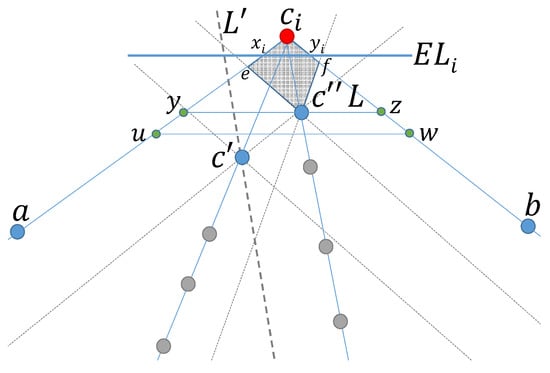
Figure 3. Eligible area computation; the shaded area depicts $EA\left(c_i\right)$.

Lemma 1

(Reference [9]). The eligible area $EA\left(c_i\right)$ for each corner $c_i$ of $\mathbf{P}$ is bounded by a non-empty convex polygon. Moreover, when $c_i$ moves to a point inside $EA\left(c_i\right)$, then $c_i$ remains as a corner of $\mathbf{P}$ and all internal and side robots of $\mathbf{P}$ are visible to $c_i$ (and vice versa).

It is easy to see that edges $\overline{c_{i}a}$ and $\overline{c_{i}b}$ are always in the perimeter of the polygonal subregion $EA\left(c_i\right)$. Let $x_i,y_i$ be two points in $\overline{c_{i}a}$ and $\overline{c_{i}b}$, respectively, that are also in the perimeter of $EA\left(c_i\right)$. Points $x_i,y_i$ can be any point in $\overline{c_{i}a}$ and $\overline{c_{i}b}$ between $c_i$ and e and $c_i$ and f, respectively, where $e,f$ are the neighbor corners of $c_i$ in $EA\left(c_i\right)$. We say line $\overline{x_i{y}_i}$ is the eligible line for $c_i$ and denote it by $E{L}_i$ (Figure 3 illustrates these ideas).

Lemma 2.

The eligible line $E{L}_i$ for each corner $c_i$ of $\mathbf{P}$ contains no point outside of $EA\left(c_i\right)$, except for the points intersecting lines from internal robots to $c_i$.

Proof. 

This lemma is immediate since the eligible area $EA\left(c_i\right)$ for each corner $c_i$ of $\mathbf{P}$ is a non-empty convex polygon (Lemma 1); hence, any line connecting any two points on the perimeter of $\mathbf{P}$ visits only the points that are in the interior of $EA\left(c_i\right)$, except for intersections with lines from internal robots to $c_i$.    □

• Convex Polygons $\mathbf{P}$, ${\mathbf{P}}^{\prime }$, ${\mathbf{P}}^{″}$, and ${\mathbf{P}}^{‴}$

$\mathbf{P}$ is the convex polygon of the points in $\mathcal{Q}$. ${\mathbf{P}}^{\prime }$ is the convex polygon connecting the corners of $\mathbf{P}$ after all of them moved to their eligible areas, $EA(*)$. ${\mathbf{P}}^{″}$ is the convex polygon with the corners of ${\mathbf{P}}^{\prime }$ and the side robots of $\mathbf{P}$ from those sides with at least two robots.

${\mathbf{P}}^{‴}$ is the convex polygon after all side points in ${\mathbf{P}}^{″}$ become corner points moving to the exterior of the side of ${\mathbf{P}}^{″}$ to which they belong. Observe that $\mathbf{P}$ contains ${\mathbf{P}}^{\prime }$ and ${\mathbf{P}}^{″}$, but not ${\mathbf{P}}^{‴}$. The left part of Figure 4 depicts $\mathbf{P}$, ${\mathbf{P}}^{\prime }$, ${\mathbf{P}}^{″}$, and the right part depicts ${\mathbf{P}}^{‴}$ formed from ${\mathbf{P}}^{″}$.

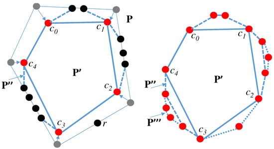
Figure 4. Example of convex polygons $\mathbf{P}$, ${\mathbf{P}}^{\prime }$, ${\mathbf{P}}^{″}$, and ${\mathbf{P}}^{‴}$.

3. Beacon-Directed Curve Positioning

The Beacon-Directed Curve Positioning framework uses robots that we call as beacons to define a curve and to guide other robots from their initial positions to final positions on the curve. The beacons start at their final positions on the curve, and all robots are $\mathcal{ASYNC}$ robots with lights. Section 4 will use the Beacon-Directed Curve Positioning framework as a tool in constructing an $\mathcal{O}\left(1\right)$ time Complete Visibility algorithm.

The destination curve is a “k-point curve” (Definition 1) that the positions of the k points can specify, so the positions of the k beacons in the framework determine.

Definition 1.

Let $\mathbb{A}\subset \mathbb{R}$ be a finite interval in the real line. Let $f:\mathbb{A}⟶\mathbb{R}$ be a (single-valued) function in which its equation $y=f\left(x\right)$ defines a curve on the plane. A k-point curve is a function f such that a set of k points $\{(x_i,f\left(x_i\right)):0\le i<k\}$ suffices to determine the constants in the equation $y=f\left(x\right)$.

For example, the curve can be a straight line that function $y=ax+c$ describes. Two points on this curve (line) enable one to determine constants a and c and so the line. As another example, the curve can be a semicircle that equation ${(y-a)}^2+{(x-b)}^2=c^2$ describes. Three points on this curve enable one to determine the constants and the curve. As another example, $c+1$ points can determine a $c$th order polynomial. Note that this section uses a global coordinate system to describe the framework, but the framework works with robots that each have only a local coordinate system.

In most robot algorithms, the movement of a robot in the move portion of an LCM cycle is along a straight line. The Beacon-Directed Curve Positioning framework assumes monotonic movement but does not require straight-line movement. So, for this section, we define a path $p_i$ in an LCM cycle of robot $r_i$ as a finite curve from initial point $(x_i,y_i)$ to final point $(x_i^{\prime },y_i^{\prime })$.

Let $f:\mathbb{A}⟶\mathbb{R}$ denote a k-point curve. Let $\mathcal{R}=\{r_i:0\le i<m\}$ denote a set of m robots with lights. The “curve positioning” goal of Beacon-Directed Curve Positioning for each $r_i$ at distinct initial point $(x_i,y_i)$ is to move $r_i$ to distinct final point $(x_i^{\prime },y_i^{\prime })=(x_i^{\prime },f\left(x_i^{\prime }\right))$ on the k-point curve. We refer to robots in $\mathcal{R}$ as “waiting robots” as they are waiting to move to the curve. The left beacons are robots $b_{\ell ,i}$, for $0\le i<k$, are initially on the curve at points with x-coordinates smaller than the x-coordinates of the final positions of all waiting robots. Similarly, right beacons are robots $b_{r,i}$, for $0\le i<k$, are initially on the curve at points with x-coordinates larger than the x-coordinates of the final positions of all waiting robots. Figure 5 depicts these concepts.

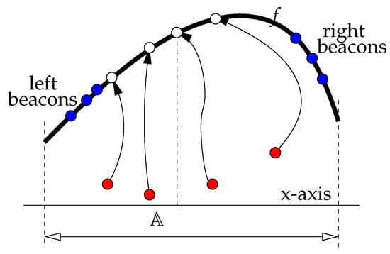
Figure 5. An illustration of Beacon-Directed Curve Positioning (BDCP). Red (resp., white) circles denote the initial (resp., final) positions of $n=4$ robots. Blue circles denote the beacons.

Definition 2.

Let $f:\mathbb{A}⟶\mathbb{R}$ be a k-point curve, and let $\mathcal{R}=\{r_i:0\le i<m\}$ be a set of waiting robots with paths $p_i$ from initial position $(x_i,y_i)$ to final position $(x_i^{\prime },f\left(x_i^{\prime }\right))$. Let ${\mathcal{B}}_{\ell }=\{b_{\ell ,i}:0\le i<k\}$, and ${\mathcal{B}}_r=\{b_{r,i}:0\le i<k\}$ be the sets of left and right beacons placed on f to the left and right of the robot set $\mathcal{R}$. Then, the triplet $⟨f,\mathcal{R},{\mathcal{B}}_{\ell }\cup {\mathcal{B}}_r⟩$ is admissible iff the following conditions hold. (a) For distinct $i,j$, paths $p_i$ and $p_j$ do not intersect. (b) For distinct $i,j$, any line through the initial position of $r_i$ intersects $p_j$ at, at most, one point. (c) For any i, a line through the initial position of $r_i$ intersects curve f (within its domain $\mathbb{A}$) at exactly one point. (d) With all robots in $\mathcal{R}$ at their initial positions, all $2k$ beacons in ${\mathcal{B}}_{\ell }\cup {\mathcal{B}}_r$ are visible to each $r_i\in \mathcal{R}$.

Definition 3.

The Beacon-Directed Curve Positioning Problem is defined as follows: Let $f:\mathbb{A}⟶\mathbb{R}$ be a k-point curve, let $\mathcal{R}=\{r_i:0\le i<m\}$, and let $\mathcal{B}$ be a set of k left and k right beacons on f such that $⟨f,\mathcal{R},\mathcal{B}⟩$ is admissible. Let the initial color of each robot $r_i\in \mathcal{R}$ bewait, and let the beacons in $\mathcal{B}$ be coloredbeacon. The objective is to move each robot $r_i\in \mathcal{R}$ to its final position on f and then change its color tobeacon.

The three condition-action pairs below present robot actions to solve the Beacon-Directed Curve Positioning Problem.

Condition 1:

Robot r has color wait, and it can see at least k robots with color beacon.

Action 1:

Robot r changes its color to not-waiting, determines the equation for the k-point curve, f, and moves monotonically on its path p to position itself on curve f.

Condition 2:

Robot r has color not-waiting.

Action 2:

Robot r changes its color to beacon.

Condition 3:

Robot r has color beacon, and it cannot see any robot colored wait.

Action 3:

Terminate.

Call as a transient robot any robot that is in motion along its path (between its initial and final positions); clearly, a transient robot was a waiting robot at the start of its cycle and is on its way to becoming a beacon at the end of its next cycle. Observe that, if a waiting robot cannot see some beacon, then there must be a transient robot that blocks its view.

We now establish conditions on the number of transient robots and the look times of waiting robots required to block the view of beacons from the waiting robots (Lemmas 3–6). Then, we will lower bound the increase in the number of beacons from one epoch to the next (Lemma 7) toward establishing an $\mathcal{O}(logk)$ epoch run time for the Beacon-Directed Curve Positioning algorithm. In the remainder of this section, we will implicitly assume in all lemmas that admissibility is satisfied; we also consider any robot with color beacon or not-waiting as a beacon. Recall that all robot movements are monotonic.

For any robot $r_i$, define the projection of $r_i$ on a k-point curve $f:\mathbb{A}⟶\mathbb{R}$ (denoted by $\mathsf{proj}\left(r_i\right)$) as the x-coordinate, $x_i^{\prime }$, of the final position of $r_i$. For a beacon b, its projection on f is $\mathsf{proj}\left(b\right)$, the x-coordinate of its position. When applied to a set $\mathcal{S}$ of robots, $\mathsf{proj}\left(\mathcal{S}\right)$ refers to the smallest interval within $\mathbb{A}$ in which the projections of all elements of $\mathcal{S}$ lie.

Lemma 3.

For left (resp., right) beacon b and waiting robot $r_i$, if a transient robot u blocks b from $r_i$, then $\mathsf{proj}\left(b\right)<\mathsf{proj}\left(u\right)<\mathsf{proj}\left(r_i\right)$ (resp., $\mathsf{proj}\left(r_i\right)<\mathsf{proj}\left(u\right)<\mathsf{proj}\left(b\right))$.

Proof. 

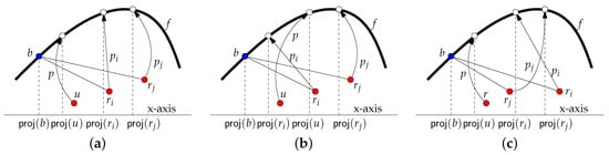
Recall that admissibility requires that paths not cross. Suppose b is a left beacon, then $\mathsf{proj}\left(b\right)<\mathsf{proj}\left(r_i\right)$. If $\mathsf{proj}\left(u\right)>\mathsf{proj}\left(r_i\right)$, then the paths of u and $r_i$ must cross (see Figure 6b), providing the necessary contradiction. The proof for a right beacon is analogous.    □

Figure 6. An illustration of the proofs of Lemmas 3 and 4: (a) illustrates no path crossing for the robots even when the transient robot u blocks the beacon b from $r_i$ and/or $r_j$ when they move, and (b,c) illustrate a path crossing scenario.

Lemma 4.

Let $\mathcal{R}=\{r_i:0\le i<m\}$ be a set of m waiting robots and let b be a left beacon with $\mathsf{proj}\left(b\right)\notin \mathsf{proj}\left(\mathcal{R}\right)$. For $0\le i<m$, let $t_i$ denote the time when $r_i$ performs its look operation. Let u be a transient robot that blocks the view of b from every waiting robot in the set $\mathcal{R}$. Then, for any distinct $0\le i,j<m$, if $\mathsf{proj}\left(b\right)<\mathsf{proj}\left(r_i\right)<\mathsf{proj}\left(r_j\right)$, then $t_i<t_j$.

Proof. 

Without loss of generality, let the x-axis be a horizontal line and let the projection of b be to the left of the projections of all elements of $\mathcal{R}$ (see Figure 6a). Since u blocks b from all robots of $\mathcal{R}$, we must have $\mathsf{proj}\left(b\right)<\mathsf{proj}\left(u\right)<\mathsf{proj}\left(r_i\right)$, for all $r_i\in \mathcal{R}$ (Lemma 3). Suppose that $\mathsf{proj}\left(r_i\right)<\mathsf{proj}\left(r_j\right)$ and $t_i>t_j$. Then, again, the paths of $r_i$ and $r_j$ will have to cross (see Figure 6c), providing the necessary contradiction.    □

Remark 1.

An analogous version of the lemma applies to a right beacon, as well.

Lemma 5.

Let $b^{\prime }$ be a right beacon and let $\mathcal{R}=\{r_i:0\le i<m\}$ be a set of m waiting robots. For $0\le i<m$, let $t_i$ denote the time when $r_i$ performs its look operation. For any distinct $0\le i,j<m$, let $\mathsf{proj}\left(r_i\right)<\mathsf{proj}\left(r_j\right)$ and let $t_i<t_j$. Then, a transient robot u can block the view of $b^{\prime }$ from at most one waiting robot from $\mathcal{R}$.

Proof. 

Suppose there exist distinct $i,j$ such that a single transient robot u blocks right beacon $b^{\prime }$ from the view of both waiting robots $r_i,r_j$. Then, $\mathsf{proj}\left(u\right)$ must lie between $\mathsf{proj}\left(b^{\prime }\right)$ and $\mathsf{proj}\left(\{r_i,r_j\}\right)$. Without loss of generality, let $\mathsf{proj}\left(r_i\right)<\mathsf{proj}\left(r_j\right)<\mathsf{proj}\left(u\right)<\mathsf{proj}\left(b^{\prime }\right)$; this implies that $t_i<t_j$ (from the lemma statement). By a result analogous to that of Lemma 4 applied to a right beacon $b^{\prime }$, we have $t_i>t_j$; this provides the necessary contradiction so that u cannot block $b^{\prime }$ from the view of more than one waiting robot.    □

Lemma 4 orders the “look-times” of waiting robots that are blocked from viewing a left beacon by a single transient robot. Given this order, Lemma 5 shows that each right beacon will have to be blocked by a different transient robot, for the same set of waiting robots. For left and right beacons $b,b^{\prime }$ and waiting robots $r_0,\dots ,r_{m-1}$, in order from left to right, observe that, at the time instant at which $r_0$ looks and transient robot u blocks b from $r_0$, some transient w blocks $b^{\prime }$ from $r_0$, and w cannot block the view of $b^{\prime }$ from $r_1,\dots ,r_{m-1}$ when they look. The following result captures this observation.

Lemma 6.

Let $b,b^{\prime }$ be left and right beacons and let $\mathcal{R}=\{r_i:0\le i<m\}$ be a set of m waiting robots. Let u be a transient robot that blocks the view of b from every waiting robot in $\mathcal{R}$. Then, at least m transient robots are needed to block $b^{\prime }$ from the view of all waiting robots of $\mathcal{R}$.

Proof. 

By Lemma 3, $\mathsf{proj}\left(b\right)<\mathsf{proj}\left(u\right)<\mathsf{proj}\left(r_i\right)$, for every $r_i\in \mathcal{R}$. Without loss of generality, let $\mathsf{proj}\left(r_i\right)<\mathsf{proj}\left(r_{i+1}\right)$, for any $0\le i<m-1$. Therefore, by Lemma 4, $t_i<t_{i+1}$; again, $t_i$ is the time when $r_i$ looks. For the right beacon $b^{\prime }$, we have $\mathsf{proj}\left(r_i\right)<\mathsf{proj}\left(r_{i+1}\right)<\mathsf{proj}\left(b^{\prime }\right)$ with $t_i<t_{i+1}$. By Lemma 5, each transient robot v can block $b^{\prime }$ from at most one element of $\mathcal{R}$. Consequently, at least $\left|\mathcal{R}\right|=m$ transient robots are needed to block $b^{\prime }$ from the view of all waiting robots of $\mathcal{R}$.    □

Next, we lower bound the increase in the number of beacons in each epoch.

Lemma 7.

If the first epoch of the algorithm started with m waiting robots and an epoch $e\ge 1$ starts with $v\ge 2k$ beacons, then epoch $e+1$ starts with at least $min\{m+2k,\frac{3v}{2}\}$ beacons.

Proof. 

The $min\{·\}$ is only to capture the idea that we cannot have more robots on f than we start out with. Blocking two different beacons, $b_i,b_j$ from the view of a given waiting robot w requires at least two transient robots. Therefore, blocking at least $v-k+1\ge k+1$ beacons from any given waiting robot (so that it sees, at most, $k-1$ beacons and fails to move during the epoch) needs at least $v-k+1$ transient robots, so the next epoch begins with at least $v-k+1$ more beacons. Observe that this is independent of the location of the beacons on f.

Thus, the number of beacons at the start of epoch $e+1$ is at least $2v-k+1>\frac{3v}{2}$ for $v\ge 2k\ge 4$.    □

Observe that ${\left(\frac{3}{2}\right)}^{\mathcal{O}(logk)}>k^2$. Therefore, from Lemma 7, in $\mathcal{O}(logk)$ epochs, all initial waiting robots have been converted to beacons. This gives the following main result of this section. We use this result in Section 4 with $k=2$ and $k=3$. For these cases, the number of epochs needed is, at most, 5 and 7, respectively.

Theorem 2.

The algorithm for the Beacon-Directed Curve Positioning Problem using a k-point curve runs on the robots with lights model in $\mathcal{O}(logk)$ epochs, using 3 colors in the $\mathcal{ASYNC}$ setting.

4. $\mathcal{O}\left(1\right)$-Time $\mathcal{ASYNC}$ Complete Visibility Algorithm

Our algorithm consists of three stages, Stages 0–2. In each stage, the robots make progress on converging toward a configuration where all the robots are in a convex hull (see Figure 7).

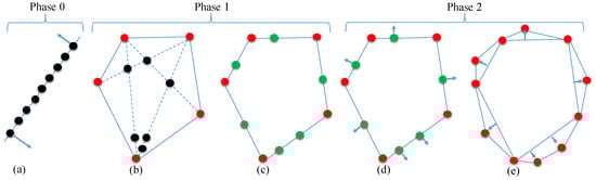
Figure 7. The three stages (or phases) of the algorithm: (a) shows an initial linear configuration in Stage 0; (b) shows either the initial non-linear configuration or when the initial linear configuration in (a) is transformed to a non-linear configuration; (c) shows the configuration of robots at the end of Stage 1, in which all the robots are on the perimeter of a convex polygon; (d) shows how the sides robots of the convex polygon moving towards the exterior of the polygon in Stage 2 to become corners of a polygon; and finally (e) shows the final configuration in Stage 2 in which all robots are on the corners of a convex polygon solving Complete Visibility.

• Stage 0 (initialization) handles the case of a collinear initial configuration. The endpoint robots move a small distance perpendicular to the line, which ensures that, in the resulting configuration, not all robots are collinear. Figure 7a and Figure 8 depict a worst case scenario, where all robots are initially collinear. In an $\mathcal{FSYNC}$ setting, this stage runs for one round [9]. In an $\mathcal{ASYNC}$ setting, we show later that this stage runs in $\mathcal{O}\left(1\right)$ epochs.
  

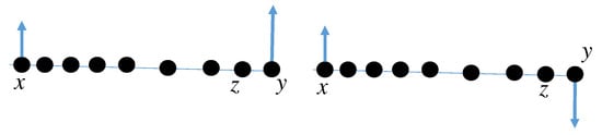  Figure 8. Examples of initially linear configurations.
• Stage 1 (interior depletion) moves all interior robots of $\mathbf{P}$ to the sides of ${\mathbf{P}}^{″}$ (Figure 7c). Stage 1 achieves this in five sub-stages, Stages 1.1–1.5, that work as follows.

  –

  Stage 1.1 starts as soon as the robots in ${\mathbf{C}}_0$ reach a non-collinear configuration (Figure 9a). Stage 1 moves the corner robots of $\mathbf{P}$ (Figure 9a) to make them corners of ${\mathbf{P}}^{\prime }$ (Figure 9b).

  

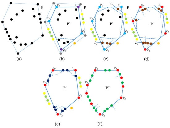  Figure 9. The five sub-stages, Stages 1.1–1.5, of Stage 1: (a) starting configuration for Stage 1, and (b–f) after Stages 1.1–1.5, respectively.

  –

  Stage 1.2 first computes the eligible lines for the corners of ${\mathbf{P}}^{\prime }$ and then moves (at least) 4 interior robots of ${\mathbf{P}}^{\prime }$ (all these robots have color start) to those eligible lines. Figure 9c illustrates this stage.

  –

  Stage 1.3 moves all the remaining interior robots of ${\mathbf{P}}^{\prime }$ to the eligible lines of the corners of ${\mathbf{P}}^{\prime }$. Figure 9d shows how the robots in the interior of ${\mathbf{P}}^{\prime }$ in Figure 9c move to $E{L}_3$.

  –

  Stage 1.4 moves the robots on the eligible lines to the sides of ${\mathbf{P}}^{\prime }$.

  Figure 9e shows how the robots on the eligible lines in Figure 9d become side robots of ${\mathbf{P}}^{\prime }$.

  –

  Stage 1.5 moves the side robots of $\mathbf{P}$ and ${\mathbf{P}}^{\prime }$ to the sides of ${\mathbf{P}}^{″}$. Figure 9f shows how the side robots of $\mathbf{P}$ and ${\mathbf{P}}^{\prime }$ in Figure 9e become side robots of ${\mathbf{P}}^{″}$.

  Stage 1 starts as soon as the robots in ${\mathbf{C}}_0$ reach to a non-collinear configuration (Figure 7b).
  In an $\mathcal{FSYNC}$ setting, this stage runs for four rounds [9]. In an $\mathcal{ASYNC}$ setting, we show later that each sub-stage runs on $\mathcal{O}\left(1\right)$ epochs and Stage 1 finishes in $\mathcal{O}\left(1\right)$ epochs.
• Stage 2 (edge depletion) relocates the side robots of ${\mathbf{P}}^{″}$ (Figure 7d) to the corners of ${\mathbf{P}}^{‴}$. Figure 7e shows the resulting convex hull. In an $\mathcal{FSYNC}$ setting, this stage runs for four rounds [9]. In an $\mathcal{ASYNC}$ setting, we show later that this stage runs for $\mathcal{O}\left(1\right)$ epochs.

At the initial configuration ${\mathbf{C}}_0$, all robots in $\mathcal{Q}$ have color start. Each robot $r_i$ works autonomously having only the information about $\mathbf{C}\left(r_i\right)$. If $\mathbf{P}\left(r_i\right)$ is a line segment and $N>3$, Stage 0 to a non-collinear ${\mathbf{C}}_0$. Stage 1 proceeds autonomously until all robots are colored either corner or side. This acts as the starting configuration for Stage 2, which proceeds autonomously until all robots have color corner for their lights. The algorithm then terminates.

The robots execute the stages sequentially one after another. One could use (only for brevity of this discussion) a different palette of colors for each stage (while keeping the number of colors used a constant). Thus, the algorithm can explicitly synchronize at the end of each stage, and our analysis can consider each stage separately. We will indicate on high level (for brevity) how robots collectively and consistently detect the end of each stage. Table 2 gives the transition of colors of the corner, side, and interior robots during the execution of the algorithm. Though robots are oblivious, the colors and configurations that the robots in $\mathcal{Q}$ assume synchronize execution of the stages (Table 3) so that robots execute stages (and sub-stages) sequentially one after another.

Table 2. Color transitions of the robots during the execution of the algorithm. A color inside $\left\{\right\}$ indicates that not all corners (sides or internals) may assume that color during the execution.

Robot	Color Transition
	start→{start_moving}→ready→ready_moving→corner1→{corner2→corner21
Corners	→corner22→corner22_moving→corner23→corner23_moving}
	→{corner3→corner4}→{corner5}→corner
	(i) start → side1 → side → {transient} → {scout1} → {scout1_moving}
Sides	→{scout2}→{beacon}→corner;
	(ii) start → side1 → special → temp_corner → corner
	start→{internal→internal_moving}→{start_moving}→{transit
Internals	→transit_moving→transit1→transit1_moving→transit2→transit2_moving
	→eligible}→{side2→side2_moving}→{side3→side3_moving}→side

Table 3. An illustration of how the colors of robots synchronize execution of the stages.

Stages	Synchronization Conditions
0 & 1.1	When Stage 0 starts, all robots have color start, and each robot sees,
	at most, two other robots collinear with it.
	When Stage 1.1 starts, all robots have color start or ready.
	Each robot sees at least two other robots not collinear with it.
1.1 & 1.2	When Stage 1.2 starts, each interior robot of ${\mathbf{P}}^{\prime }$ sees at least one robot with
	color corner2, and all corners have color corner, corner2, or corner3.
1.2 & 1.3	When Stage 1.3 starts, at least one robot has color corner4, and
	all corners have color corner, corner4, or corner5.
1.3 & 1.4	When Stage 1.4 starts, there are robots with color internal,
	internal_moving, or corner4, and at least one
	robot has color corner5.
1.4 & 1.5	When Stage 1.5 starts, the only possible robot colors are corner, side2,
	side1, and special.
1.5 & 2	When Stage 2 starts, all robots of $\mathcal{Q}$ are on the corners and sides of ${\mathbf{P}}^{″}$
	with color corner and side, respectively.
	When Stage 2 finishes, all the robots in $\mathcal{Q}$ are in the corners of ${\mathbf{P}}^{‴}$
	with color corner.

The algorithm uses 47 colors and runs for a total of $\mathcal{O}\left(1\right)$ epochs.

We showed in Sharma et al. [13] that Stages 0, 1.1, 1.4, and 2 run for $\mathcal{O}\left(1\right)$ time and Stages 1.2, 1.3, and 1.5 run for $\mathcal{O}(logN)$ time. We showed in Sharma et al. [14] that Stages 1.2, 1.3, and 1.5 can be made to run in $\mathcal{O}\left(1\right)$ time. This improvement was achieved by satisfying the conditions of the Beacon-Directed Curve Positioning framework (Section 3) to run Stages 1.2, 1.3, 1.5, and 2 in $\mathcal{O}\left(1\right)$ time; Stage 2 does not require the Beacon-Directed Curve Positioning framework as it already runs in $\mathcal{O}\left(1\right)$ time without it, but the use of the Beacon-Directed Curve Positioning framework helps to streamline the presentation of the ideas. This provides the overall $\mathcal{O}\left(1\right)$ run time for the algorithm. For Stages 1.2, 1.3, and 1.5 that use the Beacon-Directed Curve Positioning framework to run in $\mathcal{O}\left(1\right)$ time, we first describe the $\mathcal{O}(logN)$ run time ideas which are simpler to understand. The Beacon-Directed Curve Positioning framework requires each robot moving to a k-point curve to see the $2k$ beacons that are on the curve in the beginning and all the robots that move to the curve (in addition to the $2k$ beacons in the beginning) during the execution of the framework, if there is no robot currently in transit to the curve. This turned out to be particularly challenging for Stages 1.2 and 1.3, among the other conditions listed in Definition 2.

We managed to address this challenge by exploiting the eligible area $EA(*)$ of the corners of $\mathbf{P}$. Notice that all the points inside $EA\left(c_i\right)$ for each corner $c_i$ are visible to all the robots in the interior of $\mathbf{P}$ (while they are not moving). Therefore, we first develop a technique to compute an eligible line $E{L}_i$ for each corner $c_i$ of $\mathbf{P}$ by the interior robots of $\mathbf{P}$. We then develop a technique to place (at least) four interior robots on an eligible line $E{L}_i$ (note that $E{L}_i$ is inside $EA\left(c_i\right)$), two as left beacons and two as right beacons (Definition 3). After that, we develop a technique to maintain the property that the interior robots always see $c_i$ (irrespective of the robots on $E{L}_i$), and, when there is no transient robot, they see all the robots on $E{L}_i$. This idea also turned out to satisfy the remaining three conditions (Definition 2) of the Beacon-Directed Curve Positioning framework. Putting these ideas altogether achieves $\mathcal{O}\left(1\right)$ runtime for Stages 1.2 and 1.3. We then extend these techniques in the same spirit to run Stages 1.5 and 2 in $\mathcal{O}\left(1\right)$ time. We provide details of Stages 0–2 separately below and outline the major properties they satisfy.

5. Stage 0-Initialization

The goal of this stage is to transform a collinear initial configuration ${\mathbf{C}}_0$ to a non-collinear ${\mathbf{C}}_0$. Initially at ${\mathbf{C}}_0$, all $N\ge 1$ robots are stationary and have color start. Let C denote the condition that a robot x can see only one other robot y (for C to be true for x, all robots in $\mathcal{Q}$ must be collinear with x a robot at one end of the line). Otherwise, this stage is not needed since all the robots in $\mathcal{Q}$ are already on the corners, sides, and interior of a hull $\mathbf{P}$ with (at least) three corners.

If C holds, x sets its color to start_moving and moves perpendicular to line $\overline{xy}$ for a small distance $\delta$. Robot x then changes its color to ready when it becomes active next time. When at least one robot does this move, the configuration changes to a non-collinear configuration for $N>3$ (see Figure 8). The cases of $N\le 3$ can be treated separately as special cases. For $N=3$, if the robots are not collinear after at least x (or y) moved once, we already have a polygon with three corners. However, if all three robots $y,z,x$ in $\mathcal{Q}$ are again collinear after $x,y$ are moved and colored ready, the middle robot z sets its color to ready and moves orthogonal to line $\overline{xy}$ for $\delta >0$. Since $x,y$ are already colored ready, they do not make the perpendicular move again, and the move of z guarantees that the collinear configuration translates to a triangle configuration. When $N=1$, the only robot x can simply terminate since it sees no other robot. If $N=2$, one robot sees the light of other robot ready and figures out that there are only two robots in $\mathcal{Q}$ and terminates. This happens at the second (and final) round of the algorithm.

Lemma 8.

At the end of Stage 0, one of the following holds: (i) for $N=1$, the only robot simply terminates with colorstart; (ii) for $N=2$, both the robots terminate changing their color toreadyfromstart; (iii) for $N=3$, all three robots are in the vertices of a triangle with colorready; and (iv) for $N>3$, there exists a hull $\mathbf{P}$ such that all robots in $\mathcal{Q}$ are in the corners, sides, and the interior of $\mathbf{P}$ with color $\in${start,ready}.

Theorem 3.

Stage 0 finishes in (at most) three epochs.

Proof. 

For $N=1$, it is immediate that the algorithm terminates in one epoch. For $N>3$, any collinear configuration translates to a non-collinear configuration in the first epoch, since the two endpoint robots move orthogonal to the line segment in that epoch. For $N=2$, the only two robots change their color to start_moving in the first epoch. In the second epoch, they again find themselves in a line and change their color to ready. In the third epoch, each realizes that the other is the only robot in the system and terminates. For $N=3$, by the third epoch, the middle robot realizes that it is the only robot between two endpoint robots in the line segment and moves orthogonal to the line by $\delta >0$ setting its color to ready. Since the endpoint robots have color ready and do not move, this gives a non-collinear (triangle) configuration by the end of that epoch.    □

6. Stage 1-Interior Depletion

The goal of this stage is to move the corner, side, and interior robots of $\mathbf{P}$ to the corners and sides of ${\mathbf{P}}^{″}$. At the start of Stage 1, each robot is colored start or ready (Lemma 8). A robot with color ready is located at a corner of $\mathbf{P}$. A robot with color start is located at a corner or side or in the interior of $\mathbf{P}$. From Stage 0, we have that $\mathbf{P}$ is not a line segment.

Let ${\mathcal{Q}}_c,{\mathcal{Q}}_s,{\mathcal{Q}}_i$ be the sets of robots at corners, sides, and the interior of $\mathbf{P}$, respectively. For a robot $r_i$, if all other visible robots are within an angle of $<{180}^{\circ }(={180}^{\circ },>{180}^{\circ },$ respectively), then $r_i$ is a corner (side, interior, respectively) robot. Stage 1 moves robots in all ${\mathcal{Q}}_c,{\mathcal{Q}}_s,{\mathcal{Q}}_i$ to corners and sides of ${\mathbf{P}}^{″}$ and colors them as corner and side. Figure 9 illustrates Stage 1.

This stage needs four rounds in the $\mathcal{FSYNC}$ setting [9]. In Round 1.1, all corners of $\mathbf{P}$ become corners of ${\mathbf{P}}^{\prime }$ with color corner, and the side robots of $\mathbf{P}$ change their color to side1 without moving. In Round 1.2, all interior robots of $\mathbf{P}$ (also interior in ${\mathbf{P}}^{\prime }$) assume color transit moving closer to their closest corners in ${\mathbf{P}}^{\prime }$, and the robots with color side1 move to the closest sides of ${\mathbf{P}}^{\prime }$ assuming color side. In Round 1.3, some transit colored robots become side robots of ${\mathbf{P}}^{\prime }$, and, by the end of Round 1.4, all transit colored robots become side robots of ${\mathbf{P}}^{\prime }$.

Stage 1 organizes into five sub-stages in the $\mathcal{ASYNC}$ setting: Stage 1.1 translates Round 1.1, Stages 1.2, 1.3, and 1.5 translate Round 1.2, and Stage 1.4 translates Rounds 1.3 and 1.4 of the $\mathcal{FSYNC}$ algorithm. Table 3 explains how robots explicitly synchronize stages (and sub-stages) so that a next stage begins only after the current stage finishes.

• Stage 1.1 is to move the corner robots of $\mathbf{P}$ (Figure 9a) to the corners of ${\mathbf{P}}^{\prime }$ (Figure 9b) so that all interior robots of $\mathbf{P}$ see them (and vice versa). Each corner robot of $\mathbf{P}$ first moves to some point inside the eligible area in the interior of $\mathbf{P}$ and colors itself corner1. After that, each corner that has a robot in its corner triangle changes color to corner2. Otherwise, if an interior robot in present in ${\mathbf{P}}^{\prime }$, it changes color to corner3, while if no interior robot is present, it changes color to corner. The side robots of $\mathbf{P}$ first color themselves side1, and some of them later change color to special.
• Stage 1.2 is to move all the robots that are inside corner triangle $T\left(c_i\right)$ of each corner $c_i$ of ${\mathbf{P}}^{\prime }$ to the points on the corner line segment $L_i$ and color them transit. After that, the corners of ${\mathbf{P}}^{\prime }$ with color corner2 change color to corner3. Figure 9c shows how the robots inside $T\left(c_3\right)$ in Figure 9b move to $L_3$.
• Stage 1.3 is to position all the robots that are inside $\mathbf{S}\left({\mathbf{P}}^{\prime }\right)$ to the corner and triangle line segments of the corners of ${\mathbf{P}}^{\prime }$. The robots change color to transit after they reach their respective (corner or triangle) line segments. Figure 9d shows how the robots inside $\mathbf{S}\left({\mathbf{P}}^{\prime }\right)$ in Figure 9c move to triangle and corner line segments.
• Stage 1.4 is to move the robots in the corner line segments and the triangle line segments to the sides of ${\mathbf{P}}^{\prime }$. Let r be a robot on the triangle line segment $\overline{x_i{y}_i}$ of a corner $c_i$ of ${\mathbf{P}}^{\prime }$ (the case for r being on the corner line segment is analogous). Robot r moves to either $\overline{c_i{x}_i}$ or $\overline{c_i{y}_i}$ and takes color side2. Figure 9e shows how the transit robots in Figure 9d become sides of ${\mathbf{P}}^{\prime }$.
• Stage 1.5 is to make the side robots of $\mathbf{P}$ and ${\mathbf{P}}^{\prime }$ the side robots of ${\mathbf{P}}^{″}$. For this, if there is only one robot in a side of $\mathbf{P}$, it moves to the closest side in ${\mathbf{P}}^{\prime }$ and takes color side. If there are at least two robots in a side of $\mathbf{P}$, then the side robots of ${\mathbf{P}}^{\prime }$ move to the sides of ${\mathbf{P}}^{″}$ and take color side. The robots with colors side1 and special also change their color to side. Figure 9f shows how the side robots of $\mathbf{P}$ and ${\mathbf{P}}^{\prime }$ in Figure 9e become side robots of ${\mathbf{P}}^{″}$. At the end of this stage, all the robots in $\mathcal{Q}$ are on the corners and sides of ${\mathbf{P}}^{″}$ with corners colored corner and sides colored side.

In the following, we provide details of Stages 1.1–1.5 separately below and show that each stage runs for $\mathcal{O}\left(1\right)$ epochs each.

6.1. Stage 1.1-Making Corners of $\mathbf{P}$ the Corners of ${\mathbf{P}}^{\prime }$

At the start of Stage 1.1, a corner of $\mathbf{P}$ may have color ready or start. If a corner $c_i$ of $\mathbf{P}$ becomes active and has color start, then it assumes color ready. The side robots ${\mathcal{Q}}_s$ of $\mathbf{P}$ change their color to side1 from start.

Definition 4.

Let $r_a$ and $r_b$ be the counterclockwise and clockwise neighbors of a corner $c_i$ of $\mathbf{P}$ in the boundary of $\mathbf{P}$. If there are no side robots in $\overline{c_i{c}_{i-1}}$ $\left(\overline{c_i{c}_{i+1}}\right)$, then $r_a$ is $c_{i-1}$($r_b$ is $c_{i+1}$).

After $c_i$ has color ready, if it sees both $r_a,r_b$ have color $\in \{$ready, side1, corner1}, then it assumes color ready_moving and moves to a point in $EA\left(c_i\right)$. When $c_i$ becomes active next time, it is already in $EA\left(c_i\right)$, and each robot in the sets ${\mathcal{Q}}_s,{\mathcal{Q}}_i$ sees it (Lemma 1). Corner $c_i$ then changes its color to corner1. After that, $c_i$ does not move in any future epochs (but it may assume new colors).

After all corners of $\mathbf{P}$ move to their $EA(*)$, they form ${\mathbf{P}}^{\prime }$. Any robot with color side1 changes its color to special when it becomes a corner (due to the moves of corners of $\mathbf{P}$) and it sees at least one other robot with color side1 or special in the side of $\mathbf{P}$ to which it belongs. If the robot with color side1 is the only robot in that side, then it retains color side1. The robot can easily identify this situation since it is in the corridor of the side of ${\mathbf{P}}^{\prime }$ that is formed from the moves of the corners in the side of $\mathbf{P}$ to which it belongs. For example, if $s_i$ is the only side robot in a side S of $\mathbf{P}$, then it sees no other robot in the corridor of S besides itself.

Lemma 9

(Reference [9]). The interior robots of $\mathbf{P}$ remain as the interior robots of ${\mathbf{P}}^{\prime }$.

Lemma 10.

${\mathbf{P}}^{\prime }$ has the same number of corners as $\mathbf{P}$.

Proof. 

A corner $c_i$ of $\mathbf{P}$ moves to $EA\left(c_i\right)$ only after it sees both $r_a,r_b$ have color $\in \{$ready, side1, corner1}. Since the interior robots of $\mathbf{P}$ do nothing, it only remains to show that side robots of $\mathbf{P}$ remain in their original positions. This is immediate since, if $r_a$ and/or $r_b$ are side robots of $\mathbf{P}$, then they take color side1 before $c_i$ moves to $EA\left(c_i\right)$. Moreover, after $r_a$ and/or $r_b$ take color side1, they do not move to their eligible areas even if they become corners of $\mathbf{P}$. The only possibility is that $r_a,r_b$ might change their color to special.    □

Lemma 11.

The corners of $\mathbf{P}$ become corners of ${\mathbf{P}}^{\prime }$ and take colorcorner1in (at most) three epochs.

Proof. 

All the robots in the sets $R_c$ and $R_s$ (corners and sides of $\mathbf{P}$, respectively) change their colors to ready and side1, respectively, in, at most, one epoch. All the corners in $R_c$ then move to their $EA(*)$ by the end of the next epoch with color ready_moving. By the end of the third epoch, the robots that moved to $EA(*)$ change their color to corner1.    □

We now describe how the corners of ${\mathbf{P}}^{\prime }$ change their colors from corner1 to corner2, corner3, or corner. For a corner $c_i$ with color corner1, we will define conditions to be satisfied on both adjacent sides that will depend on $r_a$, its side $S_a$, and the neighboring corner on that side $c_{i-1}$ and, likewise, $r_b$, $S_b$, and $c_{i+1}$. Figure 10 shows $c_i$ (as $c_0$) and its neighboring sides $c_{i-1}$ and $c_{i+1}$ (as $w^{\prime }$ and $w^{″}$) as it moves from $\mathbf{P}$ to ${\mathbf{P}}^{\prime }$.

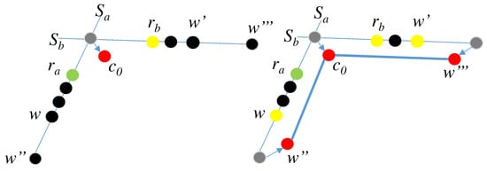
Figure 10. An illustration of how a corner $c_0$ of $\mathbf{P}$ moves during Stage 1.1.

The following lemma deals with visibility of the neighboring corners.

Lemma 12.

Corner $c_i$ of ${\mathbf{P}}^{\prime }$ sees both neighboring corners $c_{i-1}$ and $c_{i+1}$.

Proof. 

Since $c_i$, $c_{i-1}$, and $c_{i+1}$ were the endpoints of $S_a$ and $S_b$ of $\mathbf{P}$ and now moved to their $EA(*)$, the remaining side robots in $S_a$ and $S_b$ do not block the view of $c_i$ to see both $c_{i-1}$ and $c_{i+1}$. This is because $c_i$ and $c_{i-1}$ and $c_i$ and $c_{i+1}$ are not in the sides $S_a$ and $S_b$ anymore, and the interior robots of $\mathbf{P}$ remain as interior in ${\mathbf{P}}^{\prime }$ (Lemma 9).    □

Corner $c_i$ waits until $r_a$ and $c_{i-1}$ satisfy one of the conditions below for side $S_a$ and $r_b$ and $c_{i+1}$ satisfy a corresponding condition for side $S_b$.

(C1)

If $r_a$ is corner $c_{i-1}$, then $c_{i-1}$ has color ∈ {corner1, corner2, corner3, corner}.

(C2)

If $r_a$ is the only side robot on $S_a$, then $r_a$ has color side1 and $c_{i-1}$ has color ∈ {corner1, corner2, corner3, corner}.

(C3)

If $r_a$ is one of multiple side robots on $S_a$, then $r_a$ has color special and $c_{i-1}$ has color ∈ {corner1, corner2, corner3, corner}.

When the robots of both sides adjacent to $c_i$ satisfy the appropriate conditions, then $c_i$ takes a color changing action as follows. If at least one robot is inside corner triangle $T\left(c_i\right)$ (defined with respect to ${\mathbf{P}}^{\prime }$), then change color to corner2. Otherwise, if at least one robot is in the interior of ${\mathbf{P}}^{\prime }$, then change color to corner3, but, if no robot is in the interior of ${\mathbf{P}}^{\prime }$, change color to corner.

Lemma 13.

When Stage 1.1 finishes, all the corners of ${\mathbf{P}}^{\prime }$ are colored $\in \{$corner2,corner3,corner}.

Proof. 

If there is a corner of ${\mathbf{P}}^{\prime }$ with color start, ready, ready_moving, then either condition $C1$ or conditions $C2$ and $C3$ do not hold for at least one corner of ${\mathbf{P}}^{\prime }$ with color corner1, and that corner cannot change its color to corner2, corner3, or corner.    □

Lemma 14.

All corners of ${\mathbf{P}}^{\prime }$ are colored $\in \{$corner2,corner3,corner} in (at most) one epoch after they are coloredcorner1.

Proof. 

The proof is immediate since, after all corners of ${\mathbf{P}}^{\prime }$ are colored corner1, either condition $C1$ or both $C2$ and $C3$ hold for each corner of ${\mathbf{P}}^{\prime }$.    □

The corollary below follows from Lemmas 11 and 14.

Corollary 1.

Stage 1.1 finishes in (at most) four epochs.

6.2. Stage 1.2: Positioning the Robots Inside Corner Triangles of the Corners of ${\mathbf{P}}^{\prime }$ on the Corner Line Segments

Note that after Stage 1.1 finishes, the corner robots of ${\mathbf{P}}^{\prime }$ have color corner2, corner3, or corner. The side robots of $\mathbf{P}$ have color side1 or special. The interior robots of ${\mathbf{P}}^{\prime }$ have color start. We first provide an high level overview of an algorithm that finishes Stage 1.2 in $\mathcal{O}(logN)$ epochs and then provide details of an algorithm that runs Stage 1.2 in $\mathcal{O}\left(1\right)$ epochs.

The $\mathcal{O}(logN)$-epoch algorithm for Stage 1.2 works as follows. The goal is to move all the interior robots inside corner triangles to position them on the corner line segments $C{L}_i$. First, two robots are positioned on $C{L}_i$ of each triangle sequentially, if no such two robots are already on $C{L}_i$. In fact, the robots that are closest to $C{L}_i$ are chosen to perform those actions. Others remain stationary. Those robots that now moved to $C{L}_i$ are colored differently to indicate that they are on that line segment. This can be done in $\mathcal{O}\left(1\right)$ epochs. After two robots are positioned on $C{L}_i$ of each triangle and colored appropriately, the remaining robots start to move to $C{L}_i$. For a robot $r_i$ to move to $C{L}_i$, it has to correctly identify $C{L}_i$. For that, $r_i$ has to see (at least) two robots that are on $C{L}_i$. Therefore, in one epoch after two robots are positioned on $C{L}_i$, at least a robot moves to $C{L}_i$ since it sees two robots on $C{L}_i$. In the next epoch, at least a robot moves to $C{L}_i$. This makes 4 robots on $C{L}_i$. Therefore, in the third epoch, at least two robots move to $C{L}_i$, making total 6 robots. Then, $4,8,16,\dots$ number of robots can move to $C{L}_i$ in each subsequent round. Since there are n robots all internal robots may be inside a corner triangle, this whole process finishes in $\mathcal{O}(logN)$ epochs. This approach was developed in our IPDPS’17 paper [13].

We are now ready to describe $\mathcal{O}\left(1\right)$-epoch algorithm for Stage 1.2 which we developed in our SSS’17 paper [14]. We execute Stage 1.2 in two sub-stages. In Stage 1.2.1, we compute eligible lines for the corners of ${\mathbf{P}}^{\prime }$. In Stage 1.2.2, we put (at least) four interior robots in each of those lines to serve as left and right beacons as required in the Beacon-Directed Curve Positioning framework of Section 3 to run Stage 1.3 in $\mathcal{O}\left(1\right)$ epochs.

6.2.1. Stage 1.2.1-Computing Eligible Lines for the Corners of ${\mathbf{P}}^{\prime }$

Let $c_i$ be a corner of ${\mathbf{P}}^{\prime }$ colored corner2. If there are robots inside corner triangle $T\left(c_i\right)$, then pick the corner line segment $C{L}_i$; otherwise, pick the triangle line segment $T{L}_i$. Denote this line as $L_i$. We first put four interior robots of ${\mathbf{P}}^{\prime }$ in $L_i$ (Figure 11a) and color them transit. This helps later to compute the eligible line $E{L}_i$ for $c_i$.

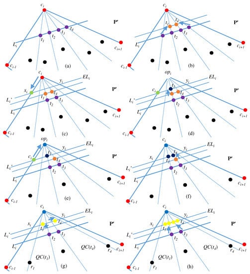
Figure 11. An illustration of how the corner and interior robots of ${\mathbf{P}}^{\prime }$ move during Stage 1.2.1.2: (a) four robots on line $L_i$ which is either a corner line segment $C{L}_i$ or a triangle line segement $T{L}_i$; (b) two robots from $L_i$ moving to a line parallel to $L_i$ towards corner $c_i$; (c) corner $c_i$ moving to $E{L}_i$ on the intersection point of $E{L}_i$ and $\overline{c_i{c}_{i-1}}$; (d) one orange robot moves to $E{L}_i$; (e) corner robot $c_i$ now moves back to the corner; (f) another orange robot moves to $E{L}_i$; (g) the orange robots on $E{L}_i$ move away from each other making room for two robots on $L_i$ to move to it; and finally (h) fours robots are on $E{L}_i$.

  Stage 1.2.1.1: Moving Four Interior Robots in ${\mathbf{P}}^{\prime }$ to $L_i$:

Let $r_i$ be the first robot to be activated among the interior robots ${\mathcal{Q}}_i$ after Stage 1.1 finishes. Suppose corner $c_i$ of ${\mathbf{P}}^{\prime }$ is closest to $r_i$. Robot $r_i$ sees $c_i$ and its neighbor corners $c_{i-1}$ and $c_{i+1}$ in ${\mathbf{P}}^{\prime }$ (Lemma 1). Therefore, $r_i$ can find whether it is inside $T\left(c_i\right)$ or not.

Suppose first that $r_i$ is inside $T\left(c_i\right)$. Let $L_{r_i}$ be the line parallel to $\overline{c_{i-1}{c}_{i+1}}$ passing through $r_i$. If there is no robot in ${\mathbf{P}}^{\prime }$ divided by $L_{r_i}$ towards $c_i$, $r_i$ changes its color to transit. Notice that, in this case, $L_{r_i}$ is in fact the corner line segment $C{L}_i$. Let $r^{″}\ne r_i$ be the robot in ${\mathcal{Q}}_i$ closest to $C{L}_i$ (w.r.t. the line parallel to $C{L}_i$) and also closest to $c_i$ (among the corners of ${\mathbf{P}}^{\prime }$). Robot $r^{″}$ changes its color to start_moving and moves to the intersection point w of $C{L}_i$ and line $\overline{c_i{r}^{″}}$. It then changes its color to transit when it becomes active next time. Until $r^{″}$ takes color transit, no other robot in ${\mathcal{Q}}_i$ moves toward $c_i$ because each robot $r^{‴}$ in ${\mathcal{Q}}_i$ closer to $c_i$ sees at least a robot with color start or start_moving in the area divided by line $L_{r^{‴}}$ (parallel to $C{L}_i)$ towards $c_i$. Similarly as $r^{‴}$, two other robots can sequentially move to $C{L}_i$ and take color transit. The remaining robots in ${\mathcal{Q}}_i$ do not move toward $c_i$ after four transit robots are in $C{L}_i$ since either they see at least a robot with color start or start_moving toward $c_i$ from their position or four transit robots already on $L_i$.

Suppose now that $r_i$ is not inside $T\left(c_i\right)$. It moves to $T{L}_i$ at the intersection point of $T{L}_i$ and $\overline{c_i{r}_i}$ assuming color start_moving and colors itself transit when it becomes active next time. The three other robots in ${\mathcal{Q}}_i$ closest to $c_i$ then move sequentially to $T{L}_i$ as the previous paragraph discussed and color themselves transit.

Corner $c_i$ changes its color to corner21 after it sees (exactly) four robots on $L_i$ with color transit. This synchronizes it with the interior robots as they also do not move to $L_i$ after four robots are already on it. After $c_i$ takes color corner21, the robots in the set ${\mathcal{Q}}_i$ (with color start) that find $c_i$ closest among the corners of ${\mathbf{P}}^{\prime }$ assume color internal (without moving). After all robots in ${\mathcal{Q}}_i$ take color internal, $c_i$ assumes color corner22 (changing from corner21). All this is possible because $c_i$ sees all the robots in ${\mathcal{Q}}_i$ (with color start), and vice versa (Lemma 1). The robots in the set ${\mathcal{Q}}_i$, after taking color internal, wait until all corners of ${\mathbf{P}}^{\prime }$ have color $\in \{$corner3, corner5, corner}. This is because they see all the corners of ${\mathbf{P}}^{\prime }$.

Observe that it is possible for some of the corners of ${\mathbf{P}}^{\prime }$ to have fewer than four robots (or even no robot) on $L_i$ even after all robots in ${\mathcal{Q}}_i$ have color internal. Those corners change their color directly to corner5 from corner2.

  Stage 1.2.1.2-Computing Eligible Lines for the Corners of ${\mathbf{P}}^{\prime }$: We describe how to compute $E{L}_i$ for $c_i$. Let $t_1,t_2,t_3,t_4$ be the four robots in $L_i$ of corner $c_i$ (Stage 1.2.1.1) with $t_2$ and $t_3$ between $t_1$ and $t_4$, and $t_2,t_3$ being closer to $t_1,t_4$, respectively (Figure 11a). We ask $t_1$ and $t_4$ to move to the lines $\overline{c_i{t}_2}$ and $\overline{c_i{t}_3}$, respectively, assuming color transit_moving. Robots $t_1,t_4$ perform this move only when they have color transit and $c_i$ has color corner22. The position they move to in those lines is the 1/8-th point from $c_i$ to $t_2$ and $t_3$, respectively. They then change their color to transit1 (Figure 11b). After $c_i$ sees both $t_1,t_4$ with color transit1, it computes $EA\left(c_i\right)$ and a point $x_i$ on $\overline{c_i{c}_{i-1}}$ (or $y_i$ on $\overline{c_i{c}_{i+1}}$) so that the line, say $L_i^{\prime }$, parallel to $\overline{t_1{t}_4}$ passing through $x_i$ (or $y_i$) crosses $EA\left(c_i\right)$. According to the construction, $\overline{t_1{t}_4}$ is parallel to $\overline{t_2{t}_3}$, and also parallel to $\overline{c_{i-1}{c}_{i+1}}$. Let $x_i$ on $\overline{c_i{c}_{i-1}}$ be the point so that $L_i^{\prime }$ crosses $EA\left(c_i\right)$. Observe that $L_i^{\prime }$ is in fact the eligible line $E{L}_i$. Corner $c_i$ then moves to $x_i$ (the procedure for $c_i$ moving to point $y_i$ is analogous) assuming color corner22_moving (Figure 11c) and changes its color to corner23. Let $o{p}_i$ be the position of $c_i$ before it moves to $x_i$.

We now describe a technique to put all $t_1,t_2,t_3,t_4$ on $L_i^{\prime }$ (which is $E{L}_i$) so that the interior robots of ${\mathbf{P}}^{\prime }$ can recognize it as $E{L}_i$. Let $t_1$ be closer to $c_i$ than $t_4$ from the new position $x_i$ of $c_i$ (the case of $t_4$ being closer to $c_i$ than $t_1$ is analogous). Robot $t_1$ moves to the intersection point of $L_i^{\prime }$ and $\overline{t_1{t}_2}$ assuming color transit1_moving (Figure 11d) and then changes its color to transit2 when it becomes active next time. After $c_i$ sees $t_1$ colored transit2, it moves back to its previous position $o{p}_i$ (where it was colored corner22) assuming color corner23_moving (Figure 11e). Although $c_i$ has no memory of $o{p}_i$, it can compute $o{p}_i$ since $o{p}_i$ is the intersection point of lines $\overline{t_1{t}_2}$ and $\overline{t_4{t}_3}$. Robot $c_i$ then assumes corner24. After this, $t_4$ with color transit1 moves to the intersection point of $L_i^{\prime }$ and $\overline{t_4{t}_3}$ assuming color transit1_moving (Figure 11f). It then assumes color transit2.

Let $o{p}_1,o{p}_4$ be the current positions of $t_1,t_4$, respectively. The robots $t_1$ and $t_4$ (after taking color transit2) move either left or right in $L_i^{\prime }$ to make room for robots $t_2$ and $t_3$ to move to $L_i^{\prime }$ without blocking any internal colored robots to see $c_i$ and also the robots $t_1,t_2,t_3,t_4$ on $L_i^{\prime }$. Robot $t_1$ (and similarly $t_4$) moves as follows. Let $\overleftrightarrow{c_i{t}_1}$ be a line that connects $t_1$ with $c_i$. Let $L^{\prime }$ be a line connecting $c_i$ with an internal colored robot r in the left or right of $\overleftrightarrow{c_i{t}_1}$ such that, in the cone area $QC\left(r\right)$ formed by $L^{\prime }$ and $\overleftrightarrow{c_i{t}_1}$, there is no other internal colored robot. Let w be the intersection point of $L_i^{\prime }$ and $L^{\prime }$. Robot $t_1$ moves to the midpoint m of the line segment that connects it with w (note that all three points $w,t_1$, and m are in $L_i^{\prime }$) assuming color transit2_moving (Figure 11g). It then changes its color to eligible when it becomes active next time. After $t_2$ and $t_3$ see both $t_1$ and $t_4$ with color eligible, $t_2$ moves to point $o{p}_1$ (the position of $t_1$ in $L_i^{\prime }$ before it moved to point m) and $t_3$ moves to $o{p}_4$ (the position of $t_4$ in $L_i^{\prime }$ before it moved) (Figure 11h). Robots $t_2,t_3$ then assume color eligible. After $c_i$ sees all $t_1,t_2,t_3,t_4$ are on $L_i^{\prime }$ with color eligible, it assumes color corner3.

Lemma 15.

During Stage 1.2.1, four interior robots of ${\mathbf{P}}^{\prime }$ inside the corner polygon $CP\left(c_i\right)$ are correctly placed on the eligible line $E{L}_i$ of $c_i$ and coloredeligibleand the corners of ${\mathbf{P}}^{\prime }$ are colored $\in \{$corner3,corner5,corner}. Stage 1.2.1 runs for $\mathcal{O}\left(1\right)$ epochs avoiding collisions and Stage 1.2.1 starts only after Stage 1.1 finishes.

Proof. 

It is easy to see that, if the robot r in the interior of ${\mathbf{P}}^{\prime }$ is not inside $CP\left(c_i\right)$, it does not move to $E{L}_i$ since r does not find $c_i$ closest to it among the corners of ${\mathbf{P}}^{\prime }$. We first show that four robots on $CP\left(c_i\right)$ correctly move to $L_i$ (which is $T{L}_i$ or $C{L}_i$) and then show that they are then correctly positioned on the eligible line $E{L}_i$.

To prove the first case, it is sufficient to show that an internal robot $r_i$ always sees its closest corner $c_i$ and two neighboring corners $c_{i-1}$ and $c_{i+1}$ of $c_i$ in ${\mathbf{P}}^{\prime }$ during Stage 1.2.1. This will allow $r_i$ to correctly compute $L_i$ and move to it if it is closer to $L_i$ than any other interior robot of ${\mathbf{P}}^{\prime }$.

Notice that $r_i$ sees all the corners of ${\mathbf{P}}^{\prime }$ in the beginning of Stage 1.2.1 as no robot has moved to lines $C{L}_i$ or $T{L}_i$ at that time. Let $r_{i-1},r_{i+1}$ be the closest interior robots to corners $c_{i-1},c_{i+1}$, respectively. Let $r_{i-1}$ ($r_{i+1}$) be currently moving or have moved to $L_{i-1}$ ($L_{i+1}$). We will show that $r_{i-1},r_{i+1}$ do not block $r_i$ to see $c_{i-1},c_{i+1}$, respectively. Observe that, since $r_{i-1}$ ($r_{i+1}$) is currently moving to or has moved to $L_{i-1}$ ($L_{i+1}$), that means $r_{i-1}$ ($r_{i+1}$) is closer to $c_{i-1}$ ($c_{i+1}$) than any other internal robot of ${\mathbf{P}}^{\prime }$. Moreover, according to the algorithm for Stage 1.2.1.1, except $r_{i-1}$ ($r_{i+1}$), no other robot is currently moving to $c_{i-1}$ ($c_{i+1}$).

Let $L_{r_i}$ be the line parallel to $\overline{c_{i-1}{c}_{i+1}}$ passing through $r_i$. Define lines $L_{r_{i-1}},L_{r_{i+1}}$ similarly. Note that, if $r_{i-1}$ ($r_{i+1}$) is moving to or has already moved to $L_{i-1}$ ($L_{i+1}$), then no other robot with color start is inside the triangle divided by line $L_{r_{i-1}}$ ($L_{r_{i+1}}$) towards $c_{i-1}$ ($c_{i+1}$). Moreover, since the corners $c_i,c_{i-1},c_{i+1}$ have already moved to their eligible areas, a unique line connects every internal robot with these corners. Therefore, as $r_i,r_{i-1},$ and $r_{i+1}$ are moving toward different corners of ${\mathbf{P}}^{\prime }$, they do not block the view of $r_i$ to see corners $c_{i-1}$ and $c_{i+1}$. Furthermore, no more than four robots will move to $L_i$ because the interior robot in $CP\left(c_i\right)$ that is closest to $L_i$ after four robots are in $L_i$ sees all the robots in $L_i$ and, hence, simply waits.

We now show that these four robots on $L_i$ are correctly positioned on $E{L}_i$. Note that $c_i$ sees all four robots on $L_i$. Robot $c_i$ simply waits until four robots are on $L_i$. After four robots are on $L_i$, $c_i$ can wait for two of them to take color eligible. At this time, the two robots $t_1,t_4$ are on a line in the triangular area divided by line $L_i$ towards $c_i$ and the line $\overline{t_1{t}_4}$ is parallel to $L_i$ (Figure 11b). As $c_i$ now computes $EA\left(c_i\right)$ and moves to the point $x_i$ on one side $\overline{c_i{c}_{i-1}}$ (Figure 11c), the line parallel to $\overline{t_1{t}_4}$ going through $x_i$ must pass through $EA\left(c_i\right)$. Now, since the four robots are arranged on two lines $\overline{t_1{t}_4}$ and $L_i$ with two robots on each of them, they provide the bearing to move $t_1,t_4$ to $E{L}_i$. After that, the color eligible of $t_1,t_4$ will provide the bearing for $t_2,t_3$ to move to $E{L}_i$.

The colors {corner3, corner5, corner} of the corners are immediate.

We now show that Stage 1.2.1 finishes in $\mathcal{O}\left(1\right)$ epochs. The four robots can move to $L_i$ in, at most, 8 epochs, i.e., a robot takes, at most, 2 epochs. In the first epoch, a robot moves to $L_i$. In the next epoch, it changes its color to transit. After that, in one epoch, corner $c_i$ changes its color to corner21. The robots in $CP\left(c_i\right)$ then color themselves internal in one epoch. Each corner $c_i$ then colors itself corner22 or corner5 in one epoch. Therefore, Stage 1.2.1.1 finishes in, at most, 11 epochs. Similarly, since we are moving four robots on $L_i$ to $E{L}_i$, Stage 1.2.1.2 also needs $\mathcal{O}\left(1\right)$ epochs.

We now show that the execution of Stage 1.2.1 is collision-free. Note that the robots moving to two different corners do not collide since they are closer to those corners than others. The robots moving to $L_i$ in Stage 1.2.1.1 do not collide because the lines joining them with the corner $c_i$ intersect only at $c_i$ (and they do not reach $c_i$). For Stage 1.2.1.2, it is clear from the construction (see Figure 11) that the robots never share the same positions, and their paths do not cross.

Finally, since all the interior robots of $\mathbf{P}$ see all the corners of ${\mathbf{P}}^{\prime }$, the interior robots do not start Stage 1.2.1 since they see at least a robot with color corner1 until all corners of ${\mathbf{P}}^{\prime }$ are colored corner2, corner3, or corner.    □

Lemma 16.

Let $r_i$ be a robot with colorinternalin the interior of ${\mathbf{P}}^{\prime }$. When Stage 1.2.1 finishes, $r_i$ sees $c_i$ and all foureligiblecolored robots in the eligible line $E{L}_i$.

Proof. 

We have from Lemma 1 that, in the beginning of Stage 1.2, all interior robots of ${\mathbf{P}}^{\prime }$ can see $c_i$ as $c_i$ is positioned at a point inside $EA\left(c_i\right)$. Since all the interior robots of $\mathbf{P}$ can see $c_i$, a unique line joins $c_i$ with each interior robot $r_j$ of ${\mathbf{P}}^{\prime }$. Therefore, it is easy to see that two lines $\overline{c_i{r}_j}$ and $\overline{c_i{r}_k}$ joining $c_i$ with two interior robots $r_j,r_k$ of ${\mathbf{P}}^{\prime }$ intersect only at $c_i$.

In Stage 1.2.1.1, when four interior robots $t_1,\dots ,t_4$ of ${\mathbf{P}}^{\prime }$ move to $L_i$, they move in their lines $\overline{c_i{t}_j}$, $1\le j\le 4$, to reach $L_i$; hence, they do not block any other internal robot in ${\mathbf{P}}^{\prime }$ to see $c_i$ (and vice versa). Note that we consider only the robots that are colored internal (or colored start in Stage 1.2.1.1). In Stage 1.2.1.2, when $t_1,\dots ,t_4$ move to $E{L}_i$, $t_2,t_3$ move again in lines $\overline{c_i{t}_2}$ and $\overline{c_i{t}_3}$ and $t_1$ and $t_4$ move to the points of $E{L}_i$ that are not on any line $\overline{c_i{r}_k}$ joining any interior robot $r_k$ (with color internal) with $c_i$ (note that $r_k$ has not yet moved to $L_j$ or $E{L}_j$ of any corner $c_j$ of ${\mathbf{P}}^{\prime }$). Therefore, all the interior robots (with color internal) see $c_i$ even after $t_1,\dots ,t_4$ moved to $E{L}_i$.

We now show that all the interior robots of ${\mathbf{P}}^{\prime }$ see all $t_1,\dots ,t_4$ (in addition to $c_i$) after $t_1,\dots ,t_4$ are positioned on $E{L}_i$. We have from Lemma 1 that any point inside $EA\left(c_i\right)$ is visible to all the interior robots (with color internal) of ${\mathbf{P}}^{\prime }$. Moreover, since $c_i$ is already in $EA\left(c_i\right)$ due to its move in Stage 1.1 and $E{L}_i$ joins two points in the neighbor edges of $c_i$ in the perimeter of ${\mathbf{P}}^{\prime }$, the lines joining interior robots with $c_i$ intersect $E{L}_i$ exactly at one point, and no two interior robots of ${\mathbf{P}}^{\prime }$ are in any line $\overline{c_i{r}_j}$ of an interior robot $r_j$. Therefore, $t_1,\dots ,t_4$ are visible to all the interior robots of ${\mathbf{P}}^{\prime }$ even after that are positioned on $E{L}_i$ (and vice versa). Moreover, since $t_1,\dots ,t_4$ are in $E{L}_i$, they are colored eligible.    □

6.2.2. Stage 1.2.2: Positioning (at least) Four Interior Robots on the Eligible Lines of the Corners of ${\mathbf{P}}^{\prime }$

After computing the eligible line $E{L}_i$ for a corner $c_i$ of ${\mathbf{P}}^{\prime }$ in Stage 1.2.1, the goal in this stage is to see whether the four robots on $E{L}_i$ with color eligible can serve as left and right beacons to apply the Beacon-Directed Curve Positioning framework of Section 3 to reposition the remaining interior robots of ${\mathbf{P}}^{\prime }$ (with color internal) to the eligible lines in $\mathcal{O}\left(1\right)$ epochs. If those four robots are positioned such that all the interior robots of ${\mathbf{P}}^{\prime }$ inside the corner polygon $CP\left(c_i\right)$ are within the cone area $QC\left(c_i\right)$ formed by lines $\overleftrightarrow{c_i{t}_2},\overleftrightarrow{c_i{t}_3}$, then these robots serve as left and right beacons and this stages finishes with $c_i$ changing its color to corner4. Otherwise, (at most) four robots inside $CP\left(c_i\right)$ move to $E{L}_i$ in this stage so that two of them serve as left beacons and two of them serve as right beacons for the Beacon-Directed Curve Positioning framework. Figure 12 illustrates these ideas.

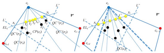
Figure 12. An illustration of how the interior robots of ${\mathbf{P}}^{\prime }$ move to the eligible lines during Stage 1.2.2.

The details are as follows. Let $r_i$ be the first robot with color internal to be activated after all the corners of ${\mathbf{P}}^{\prime }$ are colored corner3, corner5, or corner with at least a corner colored corner3. Let $r_i$ be closest to corner $c_i$ of ${\mathbf{P}}^{\prime }$ than any other corner of ${\mathbf{P}}^{\prime }$. Robot $r_i$ sees $c_i$ (Lemma 16) which has color corner3. Robot $r_i$ also sees both the neighboring corners $c_{i-1},c_{i+1}$ of $c_i$ in ${\mathbf{P}}^{\prime }$ and eligible colored robots $t_1,t_2,t_3,t_4$ that are on the eligible line $E{L}_i$ of $c_i$ (Lemma 16).

Let $Q{C}^{\prime }\left(r_i\right)$ be the cone area of ${\mathbf{P}}^{\prime }$ formed by line $\overleftrightarrow{c_i{r}_i}$ and side $\overline{c_i{c}_{i-1}}$ of ${\mathbf{P}}^{\prime }$; the left of Figure 12 shows the cone areas $Q{C}^{\prime }\left(r_3\right)$ and $Q{C}^{\prime }\left(r_4\right)$ of two internal robots $r_3$ and $r_4$. $Q{C}^{″}\left(r_i\right)$ for $r_i$ formed by lines $\overleftrightarrow{c_i{r}_i}$ and $\overline{c_i{c}_{i+1}}$ can be defined similarly; the left of Figure 12 also shows $Q{C}^{″}\left(r_1\right)$ and $Q{C}^{″}\left(r_2\right)$ of two internal robots $r_1$ and $r_2$. If there is no other robot with color internal in $Q{C}^{\prime }\left(r_i\right)$ (and/or $Q{C}^{″}\left(r_i\right)$) that is closer to $c_i$ than $r_i$, then $r_i$ moves to $E{L}_i$ at the intersection point of $E{L}_i$ and $\overline{c_i{r}_i}$ assuming color internal_moving. As depicted in the left of Figure 12, $r_1$ does not see any other robot closer to $c_i$ in $Q{C}^{″}\left(r_1\right)$ and moves to $E{L}_i$. It then assumes color eligible when it becomes active next time.

Robot $r_i$ determines whether there is some other robot $r_j$ in the cone area $Q{C}^{\prime }\left(r_i\right)$ (and/or $Q{C}^{″}\left(r_i\right)$) that is closer to $c_i$ than itself as follows. Let $L^{\prime },L^{″}$ be two lines perpendicular to $\overline{c_i{c}_{i-1}}$ and $\overline{c_i{c}_{i+1}}$, respectively, passing through their midpoints, forming the convex polygon $CP\left(c_i\right)$. If there is a robot $r_j$ with color internal in $Q{C}^{\prime }\left(r_i\right)$ ($Q{C}^{″}\left(r_i\right)$) divided by line $L^{\prime }$ ($L^{″}$) towards $c_i$, then $r_i$ assumes that $r_j$ is closer to $c_i$ in $Q{C}^{\prime }\left(r_i\right)$ ($Q{C}^{″}\left(r_i\right)$).

Note that $r_i$ always sees $c_i$ (Lemma 16). However, $r_i$ may not see $c_{i-1}$ or $c_{i+1}$ when there is another robot $r^{\prime }$ in $CP\left(c_i\right)$ that it currently transient to $E{L}_i$. Nevertheless, observe that the robots moving to $E{L}_{i-1}$ and $E{L}_{i+1}$ do not block the view of $r_i$ to see $c_{i-1}$ and $c_{i+1}$. Therefore, $r_i$ decides to move to $E{L}_i$ if and only if the first robot it sees in both the left and right of $c_i$ has color $\in \{$corner3, corner4, corner5, corner}. Finally, when $r_i$ sees two robots with color eligible in its cone area $Q{C}^{\prime }\left(r_i\right)$ (and/or $Q{C}^{″}\left(r_i\right)$), it does not move to $E{L}_i$ (even if there is no other robot $r^{\prime }$ closer to $c_i$ in $Q{C}^{\prime }\left(r_i\right)$ and/or $Q{C}^{″}\left(r_i\right)$ than itself).

As soon as the corner $c_i$ sees (at least) four eligible robots in $E{L}_i$, it assumes color corner4 if the following holds. Let $t^{\prime }$ ($t^{″}$) be the second robot in $E{L}_i$ from the either end $x_i,y_i$ of $E{L}_i$ (Figure 12). Let $QC\left(c_i\right)$ be the cone area formed by lines $\overleftrightarrow{c_i{t}^{\prime }}$ and $\overleftrightarrow{c_i{t}^{″}}$ (the area between two thick dotted lines in the right of Figure 12). If all the robots with color internal inside the corner polygon $CP\left(c_i\right)$ lie within $QC\left(c_i\right)$, $c_i$ assumes color corner4. The right of Figure 12 illustrates these ideas, where all the internal robots (shown as black) are within $QC\left(c_i\right)$.

Lemma 17.

Let there be at least foureligiblecolored robots on $E{L}_i$. All the robots with colorinternalinside the corner polygon $CP\left(c_i\right)$ see $c_i$ and the robots on $E{L}_i$. Furthermore, $c_i$ sees all the robots on $E{L}_i$.

Proof. 

The proof is to extend the argument of Lemma 16 for the robots that move to $E{L}_i$ during Stage 1.2.2. We have from Lemma 16 that the points on $E{L}_i$ are visible to all the interior robots of $\mathbf{P}$. Moreover, since any interior robot $r_j$ moves to $E{L}_i$ following the line $\overline{c_i{r}_j}$ joining $c_i$ with $r_j$, it does not block the visibility of $c_i$ to see the robots inside $CP\left(c_i\right)$. Moreover, $c_i$ sees all the robots on $E{L}_i$ since there is no other robot in the interior of ${\mathbf{P}}^{\prime }$ divided by $E{L}_i$ towards $c_i$.    □

Observe that it is possible for some corner $c_j$ of ${\mathbf{P}}^{\prime }$ to not have (at least) four eligible robots in $E{L}_j$ even after all the robots inside $CP\left(c_j\right)$ moved to $E{L}_j$. In this case, $c_j$ assumes color corner5 (directly from corner3). Observe also that there can be, at most, eight robots on $E{L}_i$ before any corner $c_i$ changes its color to corner4 since all four robots $t_1,t_2,t_3,t_4$ that are positioned on $E{L}_i$ in Stage 1.2.1.2 are such that they are positioned within $QC\left(c_i\right)$ and four new robots inside $CP\left(c_i\right)$ need to be moved to $E{L}_i$ so that there will be two robots to act as left beacons and two robots to act as right beacons on $E{L}_i$. This configuration is needed for an admissible configuration for Stage 1.3.

Lemma 18.

During Stage 1.2.2, (at least) four internal robots of ${\mathbf{P}}^{\prime }$ are positioned on the eligible lines and coloredeligible. Stage 1.2.2 runs for $\mathcal{O}\left(1\right)$ epochs avoiding collisions and Stage 1.2.2 starts only after Stage 1.2.1 finishes.

Proof. 

We have from Lemma 16 that, when Stage 1.2.1 finishes, any robot with color internal in the interior of ${\mathbf{P}}^{\prime }$ sees $c_i$ and all four eligible colored robots on $E{L}_i$. Robot $r_i$ also sees $c_{i-1}$ and $c_{i+1}$ if no robot is currently in transit to $E{L}_i$ (irrespective of the interior robots in transit to $E{L}_{i-1}$ and $E{L}_{i+1}$). Note that only the robots inside $CP\left(c_i\right)$ move to $c_i$ since, otherwise, they will be closest to some other corner of ${\mathbf{P}}^{\prime }$ than $c_i$. Therefore, any robot $r_i$ inside $CP\left(c_i\right)$ can see all $c_i,c_{i-1},c_{i+1}$ if no robot inside $CP\left(c_i\right)$ is currently in transit to $E{L}_i$ (Lemma 17). Therefore, $r_i$ can compute the cone areas $Q{C}^{\prime }\left(r_i\right)$ and $Q{C}^{″}\left(r_i\right)$. Moreover, since $r_i$ sees all $c_i,c_{i-1},c_{i+1}$, it can find whether there is some robot inside cone $Q{C}^{\prime }\left(r_i\right)$ and/or $Q{C}^{″}\left(r_i\right)$. Therefore, $r_i$ can correctly move to $E{L}_i$.

We now show that Stage 1.2.2 runs for $\mathcal{O}\left(1\right)$ epochs. Note that since four robots are already on $E{L}_i$ due to the execution in Stage 1.2.1, at most, four new robots move to $E{L}_i$ at Stage 1.2.2. A robot can move to $E{L}_i$ in two epochs; hence, it needs eight rounds to put four new robots on $E{L}_i$. After that, the corner $c_i$ can color itself corner4 in one epoch.

The execution is collision-free since the robots moving to different eligible lines do not collide. Moreover, the robots moving to the same eligible line also do not collide since the straight lines (joining them with $c_i$) they follow to reach $E{L}_i$ do not intersect before $c_i$.

Finally, Stage 1.2.2 starts only after Stage 1.2.1 finishes because the robots in the interior of ${\mathbf{P}}^{\prime }$ with color internal see at least a corner with color $\notin \{$corner3, corner5, corner} during Stage 1.2.1.    □

6.3. Stage 1.3-Positioning the Remaining Internal Robots of ${\mathbf{P}}^{\prime }$ on the Eligible Lines

In the beginning of Stage 1.3, all corners of ${\mathbf{P}}^{\prime }$ have color $\in \{$corner4, corner5, corner} with at least a corner colored corner4 (otherwise, there is no interior robot with color internal in ${\mathbf{P}}^{\prime }$).

Using the $\mathcal{O}(logN)$-epoch approach developed in IPDPS’17 [13], all interior robots of ${\mathbf{P}}^{\prime }$ that are on the corner line segments have color eligible and the rest have color internal. The goal is to move the internal colored robots to position themselves on the corner line segments. This is done as follows: Each robot colored internal find the closest corner of ${\mathbf{P}}^{\prime }$. It then moves toward that corner to be positioned on the corner line segment if it sees at least twp robots that are positioned on that corner line segment with color eligible. The $\mathcal{O}(logN)$-epoch argument for this approach is in the lines of the argument we provided in Stage 1.2.

We now describe the $\mathcal{O}\left(1\right)$-epoch approach developed in SSS’17 [14]. At the end of Stage 1.2, all interior robots of ${\mathbf{P}}^{\prime }$ that are on the eligible lines have color eligible and the rest have color internal. Let $c_i$ be a corner of ${\mathbf{P}}^{\prime }$ colored corner4, and let r be a robot with color internal that is inside the corner polygon $CP\left(c_i\right)$. Note that r is closer to $c_i$ than other corners of ${\mathbf{P}}^{\prime }$ and it always sees $c_i$ (Lemma 16). Robot r moves as follows.

Condition 1.3.1:

Robot r has color internal and it can see at least two eligible colored robots towards $c_i$.

Action 1.3.1:

Let $L_r$ be the line formed by those eligible robots. Robot r assumes color internal_moving and moves to the intersection point w of lines $L_r$ and $\overline{c_{i}r}$.

Condition 1.3.2:

Robot r has color internal_moving.

Action 1.3.2:

Robot r assumes color eligible.

As soon as $c_i$ does not see any robot with color internal or internal_moving (i.e., all robots in the interior of ${\mathbf{P}}^{\prime }$ are placed in the eligible lines), it assumes color corner5. We can prove the following two lemmas.

Lemma 19.

During Stage 1.3, theeligiblecolored robots positioned on $E{L}_i$ of a corner $c_i$ of ${\mathbf{P}}^{\prime }$ are seen by all theinternalcolored robots inside $CP\left(c_i\right)$ (and vice versa), if there is no transient robot towards $E{L}_i$.

Proof. 

We have from Lemmas 16 and 17 that the robots inside $CP\left(c_i\right)$ see all the robots on $E{L}_i$ at the end of Stage 1.2. The direct extension of those lemmas shows that, if a robot inside $CP\left(c_i\right)$ moves to $E{L}_i$, it will also be visible to the remaining robots inside $CP\left(c_i\right)$ waiting to move to $E{L}_i$. Therefore, if some interior robot $r_l$ inside $CP\left(c_i\right)$ does not see any robot $r_e$ on $E{L}_i$, then there must be some robot $r_f$ that is blocking the view of $r_e$ from $r_l$. Since the interior robots do not block the view while they are waiting to move to $E{L}_i$, there must be a robot currently in transit to $E{L}_i$.    □

Lemma 20.

During Stage 1.3, all the robots in the interior of ${\mathbf{P}}^{\prime }$ (with colorinternal) are correctly positioned on the eligible lines of the corners of ${\mathbf{P}}^{\prime }$ and coloredeligible. Moreover, the corners of ${\mathbf{P}}^{\prime }$ are coloredcorner5. Furthermore, Stage 1.3 runs for $\mathcal{O}\left(1\right)$ epochs avoiding collisions and Stage 1.3 starts only after Stage 1.2.2 finishes.

Proof. 

The idea is to show that the configuration at the end of Stage 1.2 satisfies all the conditions of Definition 2 to apply the Beacon-Directed Curve Positioning framework of Section 3 to run this stage in $\mathcal{O}\left(1\right)$ epochs. We have that the final positions of the robots inside $CP\left(c_i\right)$ on the eligible line $E{L}_i$ (a 2-point curve) are in the positions enclosed within the cone area $QC\left(c_i\right)$ and two eligible robots (that serve as left beacons) are in the left of $QC\left(c_i\right)$ and two eligible robots (that serve as right beacons) are in the right of $QC\left(c_i\right)$. We argue that all four conditions of Definition 2 are satisfied in Stage 1.3. Condition (a) is satisfied since the paths $p_i,p_j$ of two different robots $r_i,r_j$ in the interior of $CP\left(c_i\right)$ do not intersect while moving to $E{L}_i$. Condition (b) is also satisfied since the robots move in straight lines joining them with $c_i$. Condition (c) is satisfied since the paths $p_i,p_j$ intersect $E{L}_i$ at one point. Finally, Condition (d) is also satisfied since all four beacons are visible to each robot $r_i$ in their initial positions (Lemma 17). Therefore, due to Theorem 2, Stage 3 runs in $\mathcal{O}\left(1\right)$ epochs.

The execution is collision-free since the paths of any two robots do not intersect and they do not land up in the same position in $E{L}_i$.

Finally, Stage 1.3 starts only after Stage 1.2 finishes because the remaining robots in the interior of ${\mathbf{P}}^{\prime }$ do not see $c_i$ colored corner4 until Stage 1.2 finishes.    □

6.4. Stage 1.4-Positioning the Robots on the Eligible Line to the Sides of ${\mathbf{P}}^{\prime }$

Let r be a robot on the corner line segment $L_i$ or the triangle line segment $\overline{x_i{y}_i}$. Note that, if there are robots in $L_i$, then there are no robots in $\overline{x_i{y}_i}$ (and vice versa). Therefore, for simplicity, we denote by $\overline{x_i{y}_i}$ both the corner and triangle line segments of $c_i$. The goal is to move r to a position on side $\overline{c_i{c}_{i-1}}$ or $\overline{c_i{c}_{i+1}}$ of ${\mathbf{P}}^{\prime }$ between points $c_i$ and $x_i$ ($\overline{c_i{x}_i}$) or $c_i$ and $y_i$ ($\overline{c_i{y}_i}$). At the end of Stage 1.4, all the transit colored robots are on the sides of ${\mathbf{P}}^{\prime }$ with color side2. To move robots on $\overline{x_i{y}_i}$ to $\overline{c_i{x}_i}$ or $\overline{c_i{y}_i}$, each robot on $\overline{x_i{y}_i}$ should be able to recognize sides $\overline{c_i{c}_{i-1}}$ and $\overline{c_i{c}_{i+1}}$ of ${\mathbf{P}}^{\prime }$.

Let $y_{i-1}$ and $x_{i+1}$ be the points in sides $\overline{c_i{c}_{i-1}}$ and $\overline{c_i{c}_{i+1}}$ at distance $\mathsf{length}\left(\overline{c_i{c}_{i-1}}\right)/8$ and $\mathsf{length}\left(\overline{c_i{c}_{i+1}}\right)/8$ from $c_{i-1}$ and $c_{i+1}$, respectively. It is easy to show that each robot on $\overline{x_i{y}_i}$ sees all robots that are positioned on $\overline{c_i{c}_{i-1}}$ and $\overline{c_i{c}_{i+1}}$ between points $x_i$ and $y_{i-1}$ and $y_i$ and $x_{i+1}$. Therefore, we first move two robots on (i) $\overline{x_i{y}_i}$ and $\overline{x_{i+1}{y}_{i+1}}$ to $\overline{y_i{x}_{i+1}}$ and (ii) $\overline{x_i{y}_i}$ and $\overline{x_{i-1}{y}_{i-1}}$ to $\overline{x_i{y}_{i-1}}$ and color them side2. After that, all robots in $\overline{x_i{y}_i}$ can move to $\overline{c_i{x}_i}$ or $\overline{c_i{y}_i}$. Figure 13 illustrates the ideas of this stage.

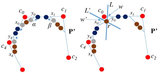
Figure 13. An illustration of how robots on $E{L}_i$ move to the sides of ${\mathbf{P}}^{\prime }$ in Stage 1.4

Lemma 21.

Let α be the robot on $\overline{x_i{y}_i}$ and β be the robot on $\overline{x_{i+1}{y}_{i+1}}$ that are closest to side $\overline{c_i{c}_{i+1}}$ among the robots in $\overline{x_i{y}_i}$ and $\overline{x_{i+1}{y}_{i+1}}$, respectively. At least one of $\alpha ,\beta$ sees both $c_i$ and $c_{i+1}$.

Proof. 

Robot $\alpha$ can see $c_i$ as it is closest to $\overline{x_i{y}_i}$, and no robots are in the triangle $\left\{c_i{x}_i{y}_i\right\}$. Similarly, $\beta$ can see $c_{i+1}$. If $\alpha$ can also see $c_{i+1}$, then the lemma is satisfied. Otherwise, a robot on $\overline{x_{i+1}{y}_{i+1}}$ blocks the view. In that case, $\beta$, at the end of $\overline{x_{i+1}{y}_{i+1}}$, can see $c_i$ as its line of sight passes between $\alpha$ and $\overline{c_i{c}_{i+1}}$, and the lemma is satisfied.    □

Suppose $\alpha$ sees both $c_i$ and $c_{i+1}$ (the case of $\beta$ seeing $c_i$, $c_{i+1}$ is analogous). Robot $\alpha$ assumes color transit_moving and moves to the point $\rho$ at distance $\mathsf{length}\left(\overline{c_i{c}_{i+1}}\right)/4$ from $c_i$ in $\overline{c_i{c}_{i+1}}$. Then, $\alpha$ changes its color to side2. Repeat this process so that one more robot ${\alpha }^{\prime }$ places itself at point $\varrho$ at distance $\mathsf{length}\left(\overline{c_i{c}_{i+1}}\right)/4$ from $c_{i+1}$ in $\overline{c_i{c}_{i+1}}$. This robot ${\alpha }^{\prime }$ will be $\beta$ unless the next robot $\gamma$ on $\overline{x_i{y}_i}$ after $\alpha$ determines that $\beta$ cannot see $c_i$, and then ${\alpha }^{\prime }$ will be $\gamma$.

Lemma 22.

Each robot on $\overline{x_i{y}_i}$ sees the robots with colorside2placed at points ρ and ϱ of side $\overline{c_i{c}_{i+1}}$. Moreover, they see two robots placed at points ${\rho }^{\prime }$ and ${\varrho }^{\prime }$ on $\overline{c_i{c}_{i-1}}$ defined analogously to ρ and ϱ.

Proof. 

As noted above, each robot on $\overline{x_i{y}_i}$ sees all robots that are positioned on $\overline{c_i{c}_{i-1}}$ and $\overline{c_i{c}_{i+1}}$ between points $x_i$ and $y_{i-1}$ and $y_i$ and $x_{i+1}$. Robots at $\rho$, $\varrho$, ${\rho }^{\prime }$, and ${\varrho }^{\prime }$ are in these ranges.    □

Robot r in $\overline{x_i{y}_i}$, after seeing two side2 colored robots each in $\overline{c_i{c}_{i-1}}$ and $\overline{c_i{c}_{i+1}}$, moves as follows. Let L and $L^{\prime }$ be the lines perpendicular to $\overleftrightarrow{\rho \varrho }$ and $\overleftrightarrow{{\rho }^{\prime }{\varrho }^{\prime }}$ passing through r, respectively. Robot r assumes color transit_moving and moves to the intersection point w of $\overleftrightarrow{\rho \varrho }$ and L or $w^{\prime }$ of $\overleftrightarrow{{\rho }^{\prime }{\varrho }^{\prime }}$ and L, whichever is closest to it. When r becomes active next, it changes it color to side2 from transit_moving.

Lemma 23.

The robots in the corner and/or triangle line segments of ${\mathbf{P}}^{\prime }$ move to the sides of ${\mathbf{P}}^{\prime }$ and assume colorside2in $\mathcal{O}\left(1\right)$ epochs. Furthermore, Stage 1.4 starts only after Stage 1.3 finishes.

Proof. 

The movement to a side of ${\mathbf{P}}^{\prime }$ is an instance of Beacon-Directed Curve Positioning. Robots move to points $\rho$ and $\varrho$ on each side $\overline{c_i{c}_{i+1}}$ of ${\mathbf{P}}^{\prime }$ and take color side2 in, at most, four epochs. The remaining robots on corner line segments or triangle line segments move to a side of ${\mathbf{P}}^{\prime }$ and take color side2 in two more epochs.

Finally, Stage 1.4 starts only after this stage finishes since the eligible colored robots on the eligible lines see at least a robot with color internal or internal_moving until Stage 1.3 finishes. The corners can change their color to corner5 since they do not see any robot with color internal or internal_moving after all robots in the interior of ${\mathbf{P}}^{\prime }$ moved to the eligible lines of the corners of ${\mathbf{P}}^{\prime }$.    □

6.5. Stage 1.5-Making Side Robots of ${\mathbf{P}}^{\prime }$ the Side Robots of ${\mathbf{P}}^{″}$

Let S be a side of $\mathbf{P}$ with $c_i,c_{i+1}$ its endpoints. There is a side $S^{\prime }$ in ${\mathbf{P}}^{\prime }$ with $c_i,c_{i+1}$ its endpoints and all the side robots in S are in the corridor of $S^{\prime }$ with color either side1 or special. The robots that become side robots in Stage 1.4 are on $S^{\prime }$ with color side2. Stage 1.5 is for the side robots on $S^{\prime }$. Stage 1.5 starts for the side robots on $S^{\prime }$ when they do not see any other robot with color except corner, side2, side1, special.

We assume in the description below that there are at least two side robots on S and at least a side robot on $S^{\prime }$. The cases of number of robots on S and $S^{\prime }$ not satisfying this assumption can be treated as special cases and can be executed in a constant number of epochs. Let $\{s_1,s_2,\dots ,s_w\}$ be the side robots on S with $s_1$ being closer to $c_i$. Robots $s_1,s_w$ have color special and the others have side1. Since $c_i,c_{i+1}$ are endpoints of $S^{\prime }$, divide S into three sides $S_l,S_m,S_r$, where $S_l=\overline{c_i{s}_1}$, $S_m=\overline{s_1{s}_w}$, and $S_r=\overline{s_w{c}_{i+1}}$. Let $L_l,L_r$ be the lines perpendicular to $S^{\prime }$ passing through $s_1,s_w$, respectively. Let $s_1^{\prime },s_w^{\prime }$ be the intersection points of $L_l,S^{\prime }$ and $L_r,S^{\prime }$, respectively. Points $s_1^{\prime },s_w^{\prime }$ divide $S^{\prime }$ into three segments $S_l^{\prime },S_m^{\prime },S_r^{\prime }$, where $S_l^{\prime }=\overline{c_i{s}_1^{\prime }}$, $S_m^{\prime }=\overline{s_1^{\prime }{s}_w^{\prime }}$, and $S_r^{\prime }=\overline{s_w^{\prime }{c}_{i+1}}$. Figure 14 illustrates these ideas.

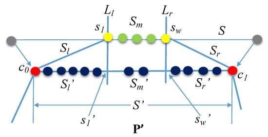
Figure 14. Example configuration of side of P and side of $P^{\prime }$ for Stage 1.5.

Recall that Stage 1.5 moves the robots on $S_l^{\prime }$, $S_m^{\prime }$, and $S_r^{\prime }$ with color side2 to $S_l$, $S_m$, and $S_r$, respectively, and colors them side.

We run two sub-stages, Stage 1.5.1 and Stage 1.5.2, one after another. In Stage 1.5.1, the robots in $S_l^{\prime },S_r^{\prime }$ move to $S_l,S_r$, respectively. In Stage 1.5.2, the robots in $S_m^{\prime }$ move to $S_m$. Stages 1.5.1 and 1.5.2 synchronize by changing the colors of $s_1,s_w$ from special to temp_corner. In both the sub-stages, the idea is to satisfy the conditions for the Beacon-Directed Curve Positioning we developed in SSS’17 to run Stage 1.5 in $\mathcal{O}\left(1\right)$ epochs. The technique we used in IPDPS’17 initially moves a robot in the first and second epochs, two robots in the third epoch, and $4,8,16,\dots$ in each subsequent epoch giving overall $\mathcal{O}(logN)$ epochs runtime for each sub-stage of Stage 1.5, in the similar spirit of the argument of this approach we outlined in Stage 1.2.

Observation 1.

During Stage 1.5.1, the robots in segment $S_m^{\prime }$ see both $s_1$ and $s_w$ with colorspecial.

6.5.1. Stage 1.5.1-Moving Robots on Segments $S_l^{\prime },S_r^{\prime }$ to $S_l,S_r$

We discuss here how robots on $S_l^{\prime }$ move to $S_l$ (the case of robots on $S_r^{\prime }$ moving to $S_r$ is analogous). Our goal is to satisfy the conditions for the framework of Section 3 to run this stage in $\mathcal{O}\left(1\right)$ epochs. In Sharma et al. [13], this stage runs in $\mathcal{O}(logN)$ epochs. Therefore, we first move four robots from $S_l^{\prime }$ to $S_l$ perpendicular to $S_l^{\prime }$ and color them side. To make sure that they serve as left and right beacons for the robots on $S_l^{\prime }$, we move two robots in $S_l^{\prime }$ closer to $c_i$ and two robots on $S_l^{\prime }$ closer to $s_1^{\prime }$ to $S_l$.

We first provide details on how we move four robots on $S_l^{\prime }$ to $S_l$. Let $s^{\prime }$ be the robot adjacent to $c_i$ in $S_l^{\prime }$. Robot $s^{\prime }$ knows $S_l$, as it sees both $c_i$ and $s_1$. Let $L^{\prime }$ be a line perpendicular to $S_l^{\prime }$ passing through $s^{\prime }$. Robot $s^{\prime }$ assumes color side2_moving and moves to the intersection point of $L^{\prime }$ and $S_l$. Robot $s^{\prime }$ then assumes color side when it becomes active next time. There are now three robots in $S_l$. The other robots on $S_l^{\prime }$ simply wait facilitating the sequential repositioning since they see a robot moving from $S_l^{\prime }$ to $S_l$. Robot $s^{″}(\ne s^{\prime })$ on $S_l^{\prime }$ that sees three robots on $S_l$ is then moved to $S_l$ similarly as $s^{\prime }$. After $s^{″}$ completes its move and assumes color side, there will be four robots on $S_l$. We then move similarly the two robots on $S_l^{\prime }$ closer to point $s_1^{\prime }$ to $S_l$ sequentially. After there are four robots on $S_l$, the robots on $S_l^{\prime }$ that see at least three robots of $S_l$ (with color side or special or corner) move to $S_l$. That is, the robots with color side, special, and corner act as left and right beacons for the robots on side $S_l^{\prime }$ with color side2. They move assuming color side3_moving and change that color to side when they become active next time. Robots on $S_l^{\prime }$ can determine that they can move to $S_l$ when they see (at least) three robots of $S_l$ since they either (i) see more than six robots of $S_l$ or (ii) if they see fewer than six robots, then there must be (at least) a robot with color side3_moving they see and this indicates that they can move. Moreover, the color side3_moving is not used in any other stage.

Since the robots on $S_r^{\prime }$ are moving to $S_r$ simultaneously with the robots on $S_l^{\prime }$ moving to $S_l$, we have to be careful that the robots of $S_l^{\prime }$ ($S_r^{\prime }$) do not move to $S_r$ ($S_l$). That is, we have to guarantee that the robots on $S_l^{\prime }$ do not mistake $S_r$ as $S_l$. This is needed for the collision-guarantee of the algorithm. We guarantee this as follows. Let X denote the set of robots with color $\in \{\mathtt{c}\mathtt{o}\mathtt{r}\mathtt{n}\mathtt{e}\mathtt{r},\mathtt{s}\mathtt{i}\mathtt{d}\mathtt{e},\mathtt{s}\mathtt{p}\mathtt{e}\mathtt{c}\mathtt{i}\mathtt{a}\mathtt{l}\}$ that the robot s on $S_l^{\prime }$ sees when it becomes active. The robots in X may be of $S_l$ or $S_r$ or both. Though $S_l$ ($S_r$) is a 2-point curve, observe that a special colored robot is at one end and a corner colored robot is at the other end also acting as beacons. Let $\left|X\right|\ge 3$; otherwise, s does not move. Let $L_l$ denote the line formed by at least three robots in X. Let $\widehat{X}$ denote the robots of X that do not belong to $L_l$. Let $L_r$ denote the line formed by the robots in $\widehat{X}$.

Let L denote the line through s perpendicular to $S_l^{\prime }$. Robot s moves to $L_l$ if and only if either of the following two conditions is satisfied.

(i)

Not all robots on $L_l$ are in the same side of L. That is, there is at least one robot of $L_l$ on the left and at least one robot of $L_l$ on the right from the point x on $L_l$ where L intersects $L_l$. This is because the robots in $L_r$ will always be on only one side of point x.

(ii)

If all the robots on $L_l$ are in the one side of L, then there is at least one robot r with color side3_moving that s sees in the other side of L (not necessarily on line $L_l$). Moreover, robot r is closer to L than any robot $r^{\prime }$ that is on line $L_r$ (w.r.t. the perpendicular distance from the robot $r^{\prime }$ on $L_r$ to L). If these conditions hold for r, then r must be either a robot of $L_l^{\prime }$ (that is already on $L_l$ or on its way to $L_l$) or the robot is at $w_1$.

Robots $s_1$ and $s_w$ assume color temp_corner as soon as all the robots on $S_l^{\prime }$ and $S_r^{\prime }$ reach to $S_l$ and $S_r$, respectively, and take color side. Observe that $s_w$ ($s_1$) sees the robots on $S_l^{\prime }$ ($S_r^{\prime }$) and the robots on $S_l$ ($S_r$) except $s_1$ ($s_w$).

Lemma 24.

During Stage 1.5.1, all the robots on $S_l^{\prime }$ and $S_r^{\prime }$ move to $S_l$ and $S_r$, respectively, and take colorside. Moreover, Stage 1.5.1 runs for $\mathcal{O}\left(1\right)$ epochs avoiding collisions, and Stage 1.5.1 starts only after Stage 1.4 finishes.

Proof. 

We prove this lemma for the robots on $S_l^{\prime }$ moving to $S_l$ (the proof for the robots on $S_r^{\prime }$ moving to $S_r$ is analogous). Until four robots are on $S_l$, the robots on $S_l^{\prime }$ move sequentially one after another to position themselves on $S_l$. Moreover, as they move perpendicular to $S_l^{\prime }$, they do not land on $S_m$ or $S_r$. After four robots are on $S_l$, we show that the robots on $S_l^{\prime }$ satisfy all the conditions of the Beacon-Directed Curve Positioning framework. Condition (a) is satisfied as the robots on $S_l^{\prime }$ always move perpendicular to $S_l^{\prime }$ to position themselves on $S_l$. Conditions (b) and (c) are also satisfied due to the perpendicular moves of the robots on $S_l^{\prime }$. Condition (d) is also satisfied as $S_l$ is a line segment and all the waiting robots on $S_l^{\prime }$ are between two left and two right beacons with color side, and the waiting robots on $S_l^{\prime }$ have color side2. Therefore, through Theorem 2, all the robots on $S_l^{\prime }$ move to $S_l$ in $\mathcal{O}\left(1\right)$ epochs.

We now show that the execution of Stage 1.5.1 is collision-free. This is immediate as in the beginning of Stage 1.5.1, no side robots are on $S_l$ or $S_r$. Moreover, the robots on $S_l^{\prime }$ are in distinct positions, and they always move perpendicularly to $S_l^{\prime }$. Therefore, the robots moving from $S_l^{\prime }$ to $S_l$ do not collide. Furthermore, as robots on $S_l^{\prime }$ do not move to $S_r$ (and vice versa), the robots from $S_l^{\prime }$ and $S_r^{\prime }$ do not collide.

Finally, Stage 1.5.1 starts only when side robots see other robots with colors only in {corner, side2, side1, special}.    □

6.5.2. Stage 1.5.2-Moving Robots on Segment $S_m^{\prime }$ to $S_m$

The robots on $S_m^{\prime }$ do not move during Stage 1.5.1. In Stage 1.5.2, similarly to Stage 1.5.1, two robots each on $S_m^{\prime }$ closer to $s_1$ and $s_w$ move to $S_m$ sequentially and take color side3. After that, the robots of $S_m^{\prime }$ that see at least two side3 robots move perpendicularly to $S_m^{\prime }$ to the line $L_m$ formed by those (at least) two side3 robots, assuming color side2_moving. The robots of $S_m^{\prime }$ after moving to $L_m$ take color side3 when they next become active. It is easy to prove that $L_m$ is in fact $S_m$. After all robots on $S_m^{\prime }$ move to $S_m$, the side robots on $S_m$ take color side and the endpoint robots of $S_m$ take color corner. As $S_m$ may already contain side robots (which are, in fact, the side robots of $\mathbf{P}$), when the robots on $S_m^{\prime }$ move, they may end up in the positions of $S_m$ that other robots already occupy. In this case, the robot moving from $S_m^{\prime }$ to $S_m$ finds the first position that is free to the left or right of the point m on $S_m$ at which a line L passing through the robot and perpendicular to $S_m^{\prime }$ intersects $S_m$. This guarantees collision freedom. Therefore, we have the following lemma.

Lemma 25.

During Stage 1.5.2, all the side robots on $S_m^{\prime }$ move to $S_m$ and take colorside, and the endpoint robots on $S_m$ take colorcorner. Moreover, Stage 1.5.2 runs for $\mathcal{O}\left(1\right)$ epochs avoiding collisions, and Stage 1.5.2 starts only after Stage 1.5.1 finishes.

Proof. 

The proof of robots in $S_m^{\prime }$ moving to $S_m$ is similar to Lemma 24.

Stage 1.5.2 starts only after Stage 1.5.1 finishes as the robots on $S_m^{\prime }$ see the colors of both $s_1$ and $s_w$ as special until all the robots on $S_l^{\prime }$ and $S_r^{\prime }$ move to $S_l$ and $S_r$, respectively.    □

Lemmas 24 and 25 provide the following corollary.

Corollary 2.

The side robots of ${\mathbf{P}}^{\prime }$ become the side robots of ${\mathbf{P}}^{″}$ and take colorsidein $\mathcal{O}\left(1\right)$ epochs.

6.6. Correctness, Collision-freedom, and Runtime for Stage 1

The correctness and collision-freedom follow similarly as in Sharma et al. [9] and the runtime follows combining Corollary 1, Lemmas 15, 18, 20, 23, and Corollary 2.

Theorem 4.

Stage 1 executes in $\mathcal{O}\left(1\right)$ epochs avoiding collisions and uses $\mathcal{O}\left(1\right)$ colors.

7. Stage 2-Edge Depletion

After Stage 1.5 finishes, all robots in $\mathcal{Q}$ are on the sides and corners of ${\mathbf{P}}^{″}$ colored side and corner, respectively. The objective of Stage 2 is to move all side robots of ${\mathbf{P}}^{″}$ to corners of ${\mathbf{P}}^{‴}$ using the Beacon-Directed Curve Positioning framework (see Figure 7d,e). The algorithm achieves this by working independently on each side $S=(c_i,s_1,s_2,\cdots ,s_m,c_{i+1})$ of ${\mathbf{P}}^{″}$, placing all side robots of S on an arc of a circle (that is, a 3-point curve) in the corridor of S that traverses the end points $c_i,c_{i+1}$ of S; call this circle a safe circle and denote it by $\mathsf{Circle}\left(S\right)$. Clearly, this ensures that no three side points of S are collinear. The algorithm further guarantees that ${\mathbf{P}}^{‴}$ is convex, thus ensuring complete visibility. Note that the technique we developed in IPDPS’17 [13] also runs Stage 2 in $\mathcal{O}\left(1\right)$ epochs without using the Beacon-Directed Curve Positioning framework; however, the use of the Beacon-Directed Curve Positioning framework streamlines the discussion as it was used in Stages 1.2, 1.3, and 1.5.

Definition 5

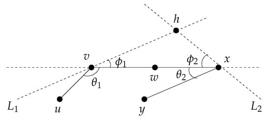
(Reference [9]). Let $u,v,w,x,y$ be points such that (a) $v,w,x$ are collinear with w between v and x, (b) $u,y$ are not collinear with line segment $\overline{vx}$, and (c) $u,y$ lie on the same side of $\overline{vx}$ such that line segments $\overline{uv}$ and $\overline{xy}$ do not intersect. Let (non-reflex) angles ${\theta }_1,{\theta }_2<{180}^{\circ }$ be ${\theta }_1=\angle (u,v,w)$ and ${\theta }_2=\angle (w,x,y)$. Let ${\varphi }_1={45}^{\circ }-\frac{{\theta }_1}{4}$ and ${\varphi }_2={45}^{\circ }-\frac{{\theta }_2}{4}$. Let $L_1$ (resp., $L_2$) be the line traversing point v (resp., x) such that it forms an angle ${\varphi }_1$ (resp., ${\varphi }_2$) with $\overline{vx}$. The point of intersection h of $L_1,L_2$ is called the “safe apex” of w w.r.t. $u,v,x,y$ and the triangle $vxh$ is called the “safe area” of $\overline{vx}$ (Figure 15).

Figure 15. An illustration of safe apex and safe area.

Stage 2 has six stages (see Figure 16). We describe the effect of these stages; Sharma et al. [9] established the correctness and collision-freedom of Stage 2 itself. Initially each side $S=(c_i,s_1,s_2,\cdots ,s_m,c_{i+1})$ has robots of color side and corner. In Stage 2.1 (the first sub-stage of Stage 2), the two extremal side robots $s_1,s_m$ (next to corners $c_i$ and $c_{i+1}$) move into the safe area of side S and become “scouts” $d_1$ and $d_m$ with color scout1 (Figure 16(1)). In Stage 2.2, each scout, $d_1$ or $d_m$, determines the circle ${\mathcal{C}}_1$ or ${\mathcal{C}}_m$ that traverses points $(c_i,d_i,c_{i+1})$ or $(c_i,d_m,c_{i+1})$, respectively.

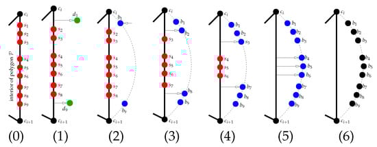
Figure 16. Stage 2 sub-stages. Part (i) shows the configuration of a side at the end of the $i^{}$th sub-stage or the beginning of the ${(i+1)}^{}$th sub-stage. The figure shows corners, side robots, scouts, and beacons as black, red, green, and blue circles.

The scout $d_x$ with the lower radius circle ${\mathcal{C}}_x$ moves to the other circle and both scouts now become “beacons” with color beacon (Figure 16(2)). The safe circle of side S (denoted by $\mathsf{Circle}\left(S\right)$) passes through both beacons $b_1$ and $b_m$ and the corners $c_i,c_{i+1}$. In Stage 2.3, the next pair of extremal points uses the corners and the two beacons to position themselves on $\mathsf{Circle}\left(S\right)$ as two more beacons $s_2$ and $s_{m-1}$ with color beacon (Figure 16(3)). Stage 2.4 similarly adds the third pair of beacons $s_3$ and $s_{m-2}$ to $\mathsf{Circle}\left(S\right)$ with color beacon (Figure 16(4)). At this point, $\mathsf{Circle}\left(S\right)$ serves as a 3-point function, and the side robots execute the Beacon-Directed Curve Positioning algorithm. Therefore, in Stage 2.5, all remaining side points, $s_4,s_5,\cdots ,s_{m-3}$ move to $\mathsf{Circle}\left(S\right)$ (Figure 16(5)). When no points remain in the interior of the polygon with color side, the beacons color themselves as corners in Stage 2.6 and the algorithm terminates (Figure 16(6)).

During Stage 2, each robot can unambiguously determine with which side S it is associated. This allows us to consider each side in isolation. We show below that this stage satisfies all the conditions required to apply the Beacon-Directed Curve Positioning framework, so it runs in $\mathcal{O}\left(1\right)$ epochs.

Lemma 26.

During Stage 2, all the side robots of ${\mathbf{P}}^{″}$ become corners of ${\mathbf{P}}^{‴}$ and take colorcorner. Stage 2 starts only after Stage 1.5.2 finishes. Moreover, Stage 2 runs for $\mathcal{O}\left(1\right)$ epochs avoiding collisions and then the algorithm terminates.

Proof. 

Stages 2.1–2.4 run in $\mathcal{O}\left(1\right)$ epochs since only, at most, two robots are moving in these stages. Stage 2.6 also runs in $\mathcal{O}\left(1\right)$ epochs as no robots move in this stage and only color computation is needed.

Therefore, it remains to show that Stage 2.5 runs in $\mathcal{O}\left(1\right)$ epochs, even by $\mathcal{ASYNC}$ robots, using the Beacon-Directed Curve Positioning framework. Observe that side S of $\mathsf{Circle}\left(S\right)$ has $1\le m<N-8$ side robots. Moreover, due to the moves of the side robots of S in Stages 2.1-2.4, six beacons are already on the safe circle, $\mathsf{Circle}\left(S\right)$.

We now argue that Stage 2.5 satisfies all the conditions required to apply the Beacon-Directed Curve Positioning technique. We first show that the waiting robots on S that are yet to move to $\mathsf{Circle}\left(S\right)$ satisfy all the conditions for an admissible configuration (Definition 2). Condition (a) is satisfied as the robots in S always move perpendicularly to S to positions on $\mathsf{Circle}\left(S\right)$. Condition (b) is also satisfied due to their perpendicular moves. Condition (c) is satisfied as the path of any robot on S perpendicular to S intersects $\mathsf{Circle}\left(S\right)$ at exactly one point, as $\mathsf{Circle}\left(S\right)$ is a circle that passes through the beacons $b_1$ and $b_m$ and the corners $c_i$ and $c_{i+1}$. Condition (d) is also satisfied as all the waiting robots are on a line S and $\mathsf{Circle}\left(S\right)$ passes through the corners $c_i$ and $c_{i+1}$ in the corridor of S. Furthermore, all the waiting robots on S are between the three left beacons and three right beacons with color beacon and the waiting robots on S have color side. Therefore, from Theorem 2, Stage 2.5 finishes in $\mathcal{O}\left(1\right)$ epochs as $k=3$ due to our use of $\mathsf{Circle}\left(S\right)$ as a curve for the final positions of the robots on S. Thus, Stage 2 runs for $\mathcal{O}\left(1\right)$ epochs. The collision-freedom in the execution of Stage 2 is immediate as the robots move perpendicularly to S. We also observe that side robots can distinguish the interior of the polygon from the outside; hence, each side S can proceed independently.

Stage 2 starts only after Stage 1.5.2 finishes as, otherwise, the robots on the sides of ${\mathbf{P}}^{″}$ with color side see at least a robot with color that is not side or corner.

The algorithm terminates after Stage 2 as all the robots have color corner after Stage 2.5 finishes and that signifies that all the robots in $\mathcal{Q}$ are on the corners of a hull $\mathbf{P}$, solving Complete Visibility.    □

Theorem 5.

Stage 2 executes in $\mathcal{O}\left(1\right)$ epochs avoiding collisions and uses 6 colors (2 colors are of Stage 1).

Proof of Theorem 1.

We have the runtime of Theorem 1 in the $\mathcal{ASYNC}$ setting combining the results of Theorems 3–5. We have the number of colors bound of Theorem 1 counting the colors listed in Table 2, which totals 47 different colors. □

8. Concluding Remarks

We have presented, to our knowledge, the first asymptotically optimal, $\mathcal{O}\left(1\right)$-time algorithm for Complete Visibility for point robots with lights using $\mathcal{O}\left(1\right)$ colors in the asynchronous setting with monotonic robot movements in a 2-dimensional real plane. The best previous results for this problem were $\mathcal{O}(logN)$ time in the fully synchronous setting and $\mathcal{O}\left(1\right)$ time for the semi-synchronous setting, both using $\mathcal{O}\left(1\right)$ colors. The result of this paper significantly improves on these existing results through new techniques as the asynchronous setting is the weakest and fully synchronous setting is the strongest among the three settings, fully synchronous, semi-synchronous, and asynchronous.

The Complete Visibility problem is fundamental with application in solving other problems under obstructed visibility. For example, the solution presented in this paper already played a crucial role in solving the pattern formation problem considered in Reference [4], where the solution was used in the first step of the four-step pattern formation algorithm. The benefit was that since the algorithm presented here arranges robots on the corners of a convex hull, we were able to exploit the knowledge of N obtained after Complete Visibility is solved to plan for how to run steps 2–4 of the pattern formation algorithm of [4].

Several questions remain open. The open questions can be categorized depending on the focus on number of colors, runtime, color/runtime trade-off, and nature of a solution. We discuss open problems in each categories below. Regarding the number of colors, a major open question is to design a 2-color algorithm (ignoring runtime) that works in the asynchronous setting even when robots have non-monotonic movements. Non-monotonic movements meaning that robots may stop before reaching the destination point or change direction before reaching the destination. The existing solutions in this direction provide a 2-color algorithm only in the case of monotonic movements in the asynchronous setting. The same can be done for the case of fat robots and design a color-optimal algorithm.

Regarding runtime, a major open question is to design a provably-efficient runtime algorithm in the asynchronous setting with non-monotonic movements. Our result in this paper only provides $\mathcal{O}\left(1\right)$ runtime with monotonic movements. First, of all, it would be interesting to see whether the algorithm of this paper can be extended to establish $\mathcal{O}(D/\Delta )$ runtime algorithm, where D is the diameter of the initial configuration and $\Delta >0$ is the minimum distance a robot travels in each move operation. $\Delta$ cannot be zero since, otherwise, the problem may not simply be solved. After that, it would be interesting to see whether the $\mathcal{O}(D/\Delta )$ bound can be improved.

Regarding trade-off, a major open question is to minimize the number of colors from current 60 to say 30 (the best possible is 2) without impacting runtime. Can we do better if we could have two lights on a robot so that it can have information on two colors for the two lights than just a single color for the single light?

Regarding nature of a solution, a major open question is to solve Complete Visibility without robots needing to be arranged on the corners of a convex hull. Can the runtime of $\mathcal{O}\left(1\right)$ can be achieved for such non-convex hull solution? What about the number of colors? What about handling non-monotonic movements? This aspect can also be considered for fat robots.

Furthermore, can the fault-tolerant algorithms be designed for Complete Visibility? There are some algorithms that handle faults in certain cases, but this direction calls for systematic effort to deal with faults under different settings. All the aforementioned aspects can be considered for robots working on a grid setting, as well.

Finally, are there other algorithms and problems that can benefit from the Beacon-Directed Curve Positioning framework the we developed in this paper?

References

- Flocchini, P.; Prencipe, G.; Santoro, N. Distributed Computing by Oblivious Mobile Robots. Synth. Lect. Distrib. Comput. Theory 2012, 3, 1–185. [Google Scholar] [CrossRef]
- Das, S.; Flocchini, P.; Prencipe, G.; Santoro, N.; Yamashita, M. Autonomous mobile robots with lights. Theor. Comput. Sci. 2016, 609, 171–184. [Google Scholar] [CrossRef]
- Peleg, D. Distributed Coordination Algorithms for Mobile Robot Swarms: New Directions and Challenges. In International Workshop on Distributed Computing; Springer: Berlin/Heidelberg, Germany, 2005; pp. 1–12. [Google Scholar]
- Vaidyanathan, R.; Sharma, G.; Trahan, J.L. On Fast Pattern Formation by Autonomous Robots. Available online: https://www.sciencedirect.com/science/article/abs/pii/S0890540121000146 (accessed on 18 January 2021).
- Di Luna, G.A.; Flocchini, P.; Chaudhuri, S.G.; Santoro, N.; Viglietta, G. Robots with Lights: Overcoming Obstructed Visibility Without Colliding. In Symposium on Self-Stabilizing Systems; Springer: Berlin/Heidelberg, Germany, 2014; pp. 150–164. [Google Scholar]
- Di Luna, G.A.; Flocchini, P.; Chaudhuri, S.G.; Poloni, F.; Santoro, N.; Viglietta, G. Mutual visibility by luminous robots without collisions. Inf. Comput. 2017, 254 Pt 3, 392–418. [Google Scholar] [CrossRef]
- Sharma, G.; Busch, C.; Mukhopadhyay, S. Mutual Visibility with an Optimal Number of Colors. In International Symposium on Algorithms and Experiments for Wireless Sensor Networks; Springer: Berlin/Heidelberg, Germany, 2015; pp. 196–210. [Google Scholar]
- Vaidyanathan, R.; Busch, C.; Trahan, J.L.; Sharma, G.; Rai, S. Logarithmic-Time Complete Visibility for Robots with Lights. In Proceedings of the 2015 IEEE International Parallel and Distributed Processing Symposium, Hyderabad, India, 25–29 May 2017; pp. 375–384. [Google Scholar]
- Sharma, G.; Vaidyanathan, R.; Trahan, J.L.; Busch, C.; Rai, S. Complete Visibility for Robots with Lights in O(1) Time. In International Symposium on Stabilization, Safety, and Security of Distributed Systems; Springer: Berlin/Heidelberg, Germany, 2016; pp. 327–345. [Google Scholar]
- Agathangelou, C.; Georgiou, C.; Mavronicolas, M. A Distributed Algorithm for Gathering Many Fat Mobile Robots in the Plane. In Proceedings of the 2013 ACM Symposium on Principles of Distributed Computing, Montreal, QC, Canada, 22–24 July 2013; pp. 250–259. [Google Scholar]
- Sharma, G.; Alsaedi, R.; Busch, C.; Mukhopadhyay, S. The Complete Visibility Problem for Fat Robots with Lights. In Proceedings of the 19th International Conference on Distributed Computing and Networking, Varanasi, India, 4–7 January 2018; pp. 21:1–21:4. [Google Scholar]
- Sharma, G.; Busch, C.; Mukhopadhyay, S. Complete Visibility for Oblivious Robots in O(N) Time. In Proceedings of the Networked Systems-6th International Conference, NETYS 2018, Essaouira, Morocco, 9–11 May 2018; pp. 67–84. [Google Scholar]
- Sharma, G.; Vaidyanathan, R.; Trahan, J.L.; Busch, C.; Rai, S. Logarithmic-Time Complete Visibility for Asynchronous Robots with Lights. In Proceedings of the 2015 IEEE International Parallel and Distributed Processing Symposium, Hyderabad, India, 25–29 May 2017; pp. 513–522. [Google Scholar]
- Sharma, G.; Vaidyanathan, R.; Trahan, J.L. Constant-Time Complete Visibility for Asynchronous Robots with Lights. In International Symposium on Stabilization, Safety, and Security of Distributed Systems; Springer: Berlin/Heidelberg, Germany, 2017; pp. 265–281. [Google Scholar]
- Di Luna, G.A.; Flocchini, P.; Poloni, F.; Santoro, N.; Viglietta, G. The Mutual Visibility Problem for Oblivious Robots. In Proceedings of the Canadian Conference on Computational Geometry, Halifax, NS, Canada, 11–13 August 2014; pp. 348–354. [Google Scholar]
- Aljohani, A.; Sharma, G. Complete Visibility for Mobile Robots with Lights Tolerating Faults. Int. J. Netw. Comput. 2018, 8, 32–52. [Google Scholar] [CrossRef]
- Poudel, P.; Aljohani, A.; Sharma, G. Fault-tolerant complete visibility for asynchronous robots with lights under one-axis agreement. Theor. Comput. Sci. 2021, 850, 116–134. [Google Scholar] [CrossRef]
- Bhagat, S.; Chaudhuri, S.G.; Mukhopadhyaya, K. Formation of General Position by Asynchronous Mobile Robots Under One-Axis Agreement. In International Workshop on Algorithms and Computation; Springer: Berlin/Heidelberg, Germany, 2016; pp. 80–91. [Google Scholar]
- Czyzowicz, J.; Gasieniec, L.; Pelc, A. Gathering Few Fat Mobile Robots in the Plane. Theor. Comput. Sci. 2009, 410, 481–499. [Google Scholar] [CrossRef]
- Adhikary, R.; Bose, K.; Kundu, M.K.; Sau, B. Mutual Visibility by Asynchronous Robots on Infinite Grid. In International Symposium on Algorithms and Experiments for Sensor Systems, Wireless Networks and Distributed Robotics; Springer: Berlin/Heidelberg, Germany, 2018; pp. 83–101. [Google Scholar]
- Sharma, G.; Vaidyanathan, R.; Trahan, J.L. Optimal Randomized Complete Visibility on a Grid for Asynchronous Robots with Lights. Int. J. Netw. Comput. 2021, 11, 607–616. [Google Scholar]
- Hector, R.; Vaidyanathan, R.; Sharma, G.; Trahan, J.L. Optimal Convex Hull Formation on a Grid by Asynchronous Robots with Lights. In Proceedings of the 2020 IEEE International Parallel and Distributed Processing Symposium, New Orleans, LA, USA, 18–22 May 2020; pp. 1051–1060. [Google Scholar]
- D’Emidio, M.; Frigioni, D.; Navarra, A. Synchronous Robots vs Asynchronous Lights-Enhanced Robots on Graphs. Electr. Notes Theor. Comput. Sci. 2016, 322, 169–180. [Google Scholar] [CrossRef][Green Version]
- Cohen, R.; Peleg, D. Local Spreading Algorithms for Autonomous Robot Systems. Theor. Comput. Sci. 2008, 399, 71–82. [Google Scholar] [CrossRef]
- Dutta, A.; Chaudhuri, S.G.; Datta, S.; Mukhopadhyaya, K. Circle Formation by Asynchronous Fat Robots with Limited Visibility. In International Conference on Distributed Computing and Internet Technology; Spring: Berlin/Heidelberg, Germany, 2012; pp. 83–93. [Google Scholar]
- Gan Chaudhuri, S.; Mukhopadhyaya, K. Leader election and gathering for asynchronous fat robots without common chirality. J. Discrete Algorithms 2015, 33, 171–192. [Google Scholar] [CrossRef]
- Honorat, A.; Potop-Butucaru, M.; Tixeuil, S. Gathering fat mobile robots with slim omnidirectional cameras. Theor. Comput. Sci. 2014, 557, 1–27. [Google Scholar] [CrossRef]
- Pagli, L.; Prencipe, G.; Viglietta, G. Getting Close Without Touching: Near-gathering for Autonomous Mobile Robots. Distrib. Comput. 2015, 28, 333–349. [Google Scholar] [CrossRef]
- Ando, H.; Suzuki, I.; Yamashita, M. Formation and agreement problems for synchronous mobile robots with limited visibility. In Proceedings of the International Conference on Distributed Computing and Internet Technology, Bhubaneswar, India, 10–13 January 1995; pp. 453–460. [Google Scholar] [CrossRef]
- Prencipe, G. Autonomous Mobile Robots: A Distributed Computing Perspective. In International Symposium on Algorithms and Experiments for Sensor Systems, Wireless Networks and Distributed Robotics; Spring: Berlin/Heidelberg, Germany, 2013; pp. 6–21. [Google Scholar]
- Yamashita, M.; Suzuki, I. Characterizing geometric patterns formable by oblivious anonymous mobile robots. Theor. Comput. Sci. 2010, 411, 2433–2453. [Google Scholar] [CrossRef]
- Abshoff, S.; Cord-Landwehr, A.; Fischer, M.; Jung, D.; Meyer auf der Heide, F. Gathering a Closed Chain of Robots on a Grid. In Proceedings of the 2016 IEEE International Parallel and Distributed Processing Symposium (IPDPS), Chicago, IL, USA, 23–27 May 2016; pp. 689–699. [Google Scholar]
- Cord-Landwehr, A.; Fischer, M.; Jung, D.; Meyer auf der Heide, F. Asymptotically Optimal Gathering on a Grid. In Proceedings of the 28th ACM Symposium on Parallelism in Algorithms and Architectures, Pacific Grove, CA, USA, 11–13 July 2016; pp. 301–312. [Google Scholar]
- Degener, B.; Kempkes, B.; Langner, T.; Meyer auf der Heide, F.; Pietrzyk, P.; Wattenhofer, R. A tight runtime bound for synchronous gathering of autonomous robots with limited visibility. In Proceedings of the Twenty-Third Annual ACM Symposium on Parallelism in Algorithms and Architectures, San Jose, CA, USA, 4–6 June 2011; pp. 139–148. [Google Scholar]
- Degener, B.; Kempkes, B.; Meyer auf der Heide, F. A local O(n2) gathering algorithm. In Proceedings of the Twenty-Second Annual ACM Symposium on Parallelism in Algorithms and Architectures, Santorini, Greece, 13–15 June 2010; pp. 217–223. [Google Scholar]
- Kempkes, B.; Kling, P.; Meyer auf der Heide, F. Optimal and competitive runtime bounds for continuous, local gathering of mobile robots. In Proceedings of the Twenty-Fourth annual ACM Symposium on Parallelism in Algorithms and Architectures, Pittsburgh, PA, USA, 25–27 June 2012; pp. 18–26. [Google Scholar]
- Izumi, T.; Potop-Butucaru, M.G.; Tixeuil, S. Connectivity-preserving Scattering of Mobile Robots with Limited Visibility. In Symposium on Self-Stabilizing Systems; Springer: Berlin/Heidelberg, Germany, 2010; pp. 319–331. [Google Scholar]
- Cord-Landwehr, A.; Degener, B.; Fischer, M.; Hüllmann, M.; Kempkes, B.; Klaas, A.; Kling, P.; Kurras, S.; Märtens, M.; Meyer auf der Heide, F.; et al. A New Approach for Analyzing Convergence Algorithms for Mobile Robots. In International Colloquium on Automata, Languages, and Programming; Springer: Berlin/Heidelberg, Germany, 2011; pp. 650–661. [Google Scholar] [CrossRef]
Publisher’s Note: MDPI stays neutral with regard to jurisdictional claims in published maps and institutional affiliations. |
© 2021 by the authors. Licensee MDPI, Basel, Switzerland. This article is an open access article distributed under the terms and conditions of the Creative Commons Attribution (CC BY) license (http://creativecommons.org/licenses/by/4.0/).