Quadratic Model-Based Dynamically Updated PID Control of CSTR System with Varying Parameters ^†

Abstract

In this paper, we discuss an improved version of the conventional PID (Proportional–Integral–Derivative) controller, the Dynamically Updated PID (DUPID) controller. The DUPID is a control solution which preserves the advantages of the PID controller and tends to improve them by introducing a quadratic error model in the PID control structure. The quadratic error model is constructed over a window of past error points. The objective is to use the model to give the conventional PID controller the awareness needed to battle the effects caused by the variation of the parameters. The quality of the predictions that the model is able to deliver depends on the appropriate selection of data used for its construction. In this regard, the paper discusses two algorithms, named 1D (one dimensional) and 2D (two dimensional) DUPID. Appropriate to their names, the former selects data based on one coordinate, whereas the latter selects the data based on two coordinates. Both these versions of the DUPID controller are compared to the conventional PID controller with respect to their capabilities of controlling a Continuous Stirred Tank Reactor (CSTR) system with varying parameters in three different scenarios. As a quantifying measure of the control performance, the integral of absolute error (IAE) metric is used. The results from the performed simulations indicated that the two versions of the DUPID controller improved the control performance of the conventional PID controller in all scenarios.

1. Introduction

To date, the PID (Proportional–Integral–Derivative) controller is the most widely used controller in industry. Certain sources indicate that it is used in up to $~$90% of the industrial plants at low control level [1,2], mainly because it is a simple, robust and cheap controller that offers good control performance in most applications. The most challenging task in PID control design is the determination of its coefficients [3,4]. Moreover, real plants are subjected to change in their parameters, i.e., parameter drift, as they operate. Hence, if the PID controller was initially designed to work for a particular operating point, after the parameters drift, the controller should be adapted to the new operating conditions. If there is no supervisory system present that automatically ensures that adaptation, one should track the parameters drift and occasionally retune the PID parameters.

To tackle the problem of changing plant parameters, adaptive control schemes are used. Among the different adaptive control schemes discussed in the literature, the most widely used is the model reference adaptive control (MRAC). This algorithm adapts the controller’s parameters with the aim to force the plant to behave as some given ideal model [5,6]. The adaptive control schemes fall into two categories [3], (i) indirect methods [5,6], and (ii) direct methods [7,8,9]. In the former, at first, a model of the plant being controlled is identified, and subsequently the obtained model is used to adjust the parameters of the PID controller. In the direct methods, the estimation of the controller parameters is carried out online so that the error between the reference model output and plant output tends to be zero. In general, these methods face difficulties emanating from two sources; one of the difficulties arises from the fact that the controlled plants are black boxes and their identification is a tough and complex task, and the second one stems from the fact that it is difficult to guarantee that the controller parameters will converge to the desired values, and achieve the goal of zero error.

Another common approach for countering the consequences of varying plant parameters found in industry is the robust control approach [10]. The ideas emerging from the development of the robust control paradigm were specialized for the case of the PID controllers, resulting in numerous tuning methods for robust PID control [11]. One of the most often used is the internal-model-based (IMC) PID robust tuning method [11,12,13]. A novel robust approach is presented in [14], to deal with the negative implications caused by the inherent feature of the IMC tuning of pole-zero cancelation. Lately, the robust control community has shifted its attention toward tuning methods based on multi-objective optimization [11,15,16]. The tuning parameters in these methods are obtained as a solution to an optimization problem which is often non-convex. The discussed robust tuning methods have proven effective in improving the robustness in a variety of control systems. However, they have certain downsides, and some of them are pinpointed as follows: firstly, in the tuning process it is necessary to account for all the parameters that can possibly vary and the bounds of their variation in advance; secondly, they usually need one or multiple linearized models of the nonlinear plant to design the controller; lastly, the methods based on optimization techniques come with a high computational burden as the optimization problem therein is non-convex.

To tackle some of the aforementioned problems, in this paper we discuss a simple and computationally non-intensive, hands-on control algorithm which is an upgraded version of the conventional PID controller—a dynamically updated PID (DUPID) control scheme [17]. This control approach uses a local quadratic model [18,19], of the plant control error to improve the robustness of the conventional PID against the change of the plant parameters. Based on this model the PID control value is adapted directly without retuning its coefficients, to steer the plant output in close proximity of the set point. The DUPID controller is mainly meant to work well for plants found in the process industry. The plants encountered there are often monotone (inert), stable and primarily affected by slow and gradual degradation in their physical components over time. The DUPID control scheme is made of two parts: a PID controller and a supervisory mechanism (SM). The SM plays the role of the adaptation mechanism; it detects the change in plant parameters by locally modelling the recent history of the control errors and uses that model to produce an incremental value that is added to the PID control value.

The control performance of the DUPID control scheme is dependent on the quality of the predictions the error model can deliver. To establish a locally precise error model, we must ensure that the data used for modelling meet certain criteria [18]. In this regard, this paper discusses two versions of the DUPID algorithm, the 1D DUPID and the 2D DUPID. The effectiveness of both versions of the DUPID controller was compared against the conventional PID controller, when each controller was applied to control the CSTR system with varying parameters [20]. We assumed that the varying parameters in question are: the heat transfer coefficient $h$ and the feed fluid temperature $T_f$. Based on this assumption we defined three different scenarios in which these parameters vary linearly over time. The observed control performance of each controller was quantified and compared against the other controllers based on the IAE metric values.

The rest of the paper is structured as follows: Firstly, the mathematical background of the PID and DUPID are presented, and the DUPID and its two versions are discussed in more detail. Secondly, the CSTR system with varying parameters is analyzed. Thirdly, the PID controller and both versions of the DUPID controller are tested when applied to the CSTR system. Finally, conclusions and an outlook for future work are given.

2. Methods

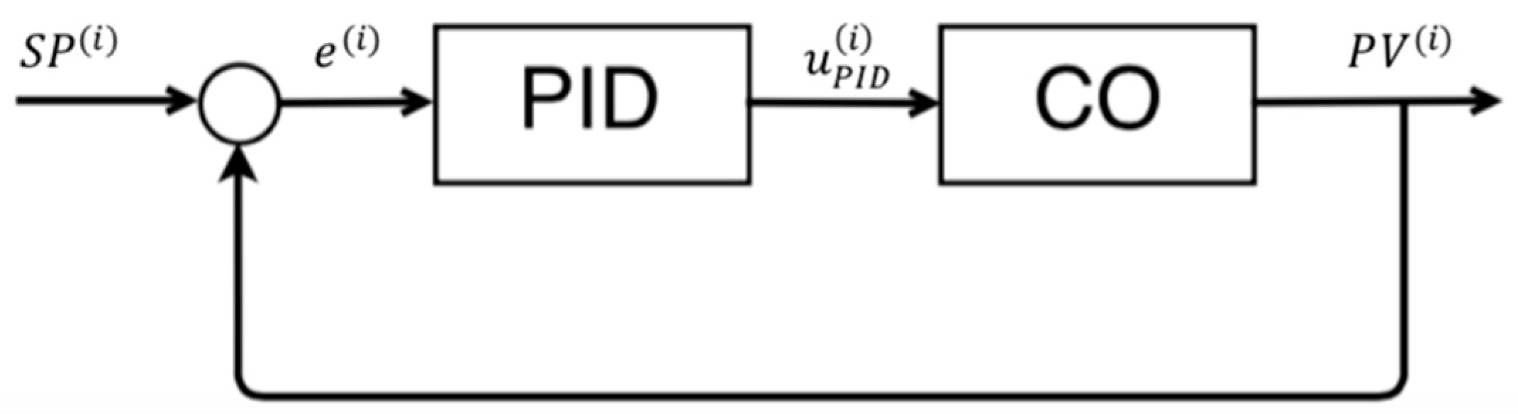
2.1. The PID Controller

In industry, more than ten particular forms of PID realizations can be found [4,21]. In this paper, the parallel PID realization is used. The mathematical definition of parallel PID realization is given with Equation (1). As it can be observed, the control value is produced in one step and it depends on the current error as well as on previous control errors. The control error in the current iteration $e^{\left(i\right)}$ is defined as the difference between the current values of the set-point (SP) and the process value (PV), $e^{\left(i\right)}=S{P}^{\left(i\right)}-P{V}^{\left(i\right)}$. The PID tuning parameters are $K_p$, $K_i$ and $K_d$, each corresponding to the P, I and D terms respectively. Finally, $u_0$ is the bias in the control signal and $T_i$ is the simulation time step:

$$u_{PID}^{\left(i\right)}=u_0+K_p{e}^{\left(i\right)} +K_i{\displaystyle \sum }_{m=1}^i{e}^{\left(m\right)}{T}_i+K_d\frac{e^{\left(i\right)}-e^{\left(i-1\right)}}{T_i}.$$

(1)

In Figure 1, the feedback control loop consisting of a PID controller and a control object (CO) is given.

2.2. The DUPID Control Scheme

The DUPID is composed of two main elements: (i) a PID controller and (ii) a supervisory mechanism (SM) (see Figure 2, dashed rectangular). The former acts as a mechanism for preserving CO stability, while the latter is responsible for calculating the incremental value $\Delta u^{\left(j\right)}$ in the PID control value. The value $\Delta u^{\left(j\right)}$ plays the role of an additional bias when the plant parameters are gradually drifting and the integral action produced by the PID controller is not enough to counter the resulting controller performance degradation caused by the varying parameters. The DUPID controller tracks the slow variation of the parameters and calculates $\Delta u^{\left(j\right)}$ which helps the PID controller to steer the plant in the direction of smaller control error.

The DUPID produces the control value in two phases: the first phase is completed after the PID control value $u_{PID}^{\left(i\right)}$ is calculated and the second is completed after $\Delta u^{\left(j\right)}$ is obtained by the SM.

With the conclusion of the second phase the aggregate control value $u_A^{\left(i\right)}$ is applied to CO, Figure 2.

$$u_A^{\left(i\right)}=u_{PID}^{\left(i\right)}+\Delta u^{\left(j\right)}$$

(2)

The term $\Delta u^{\left(j\right)}$ is generated by the SM at specific moments in time $j$, defined by the values found in the vector $DV$. The values of $DV$ are set a priori by the operator and are constant during the plant operation. The role of $DV$ is twofold: its values define the number of simulation time steps that should pass before a regression point is acquired, and at the same time its values define the frequency of $\Delta u^{\left(j\right)}$ calculation. The fundamental component of the SM is the quadratic error model given with Equation (3). The quadratic model observed here is the simplest one dimensional (one input) quadratic form:

$$E_M\left(\Delta u^{\left(j\right)},p\right)=A{\left(\Delta u^{\left(j\right)}\right)}^2+B\left(\Delta u^{\left(j\right)}\right)+C,$$

(3)

where, $p=\left\{A,B,C\right\}$ is the vector of unknown parameters and $E_M$ is the expected control error (the dependent variable). This model locally describes the functional relation between the $\Delta u^{\left(j\right)}$ and the plant control error. As new plant data are being gathered, this model is iteratively updated based on the last $N_{pp}$ point pairs $\left(\Delta u^{\left(j\right)},e_s^{\left(j\right)}\right)$, where $e_s^{\left(j\right)}$ is assigned to the $i$-th control error point $e^{\left(i\right)}$ attained at moment $j$. The objective is to use this model in iterative fashion to estimate a sequence of $\Delta u^{\left(j\right)}$ values for which the error caused by the parameters drift will be gradually decreased. To achieve this, we assume $\Delta u^{\left(j\right)}$ to be the root of the model given with Equation (3). If the roots are complex numbers, then the incremental value is calculated by differentiating Equation (3), $d{E}_M(·)/d\left(\Delta u\right)=0$. Usually, a minimum of three points is required to obtain the parameters $p$ [22]. The model based solely on the minimum required number of points has proven to be ineffective, especially when the regression data are improperly distributed or contaminated with noise [11]. These downsides can be dealt with, by choosing the number of regression points to be a compromise between the minimum required number of points and a certain threshold $\left(N_{pp}\right)$. The initial model resides on the first $N_{pp}$ points, which are gathered consecutively in $N_{pp}$ simulation time steps, as the plant is operated. Since $\Delta u^{\left(j\right)}$ does not exist at first, informative prior data are needed to establish the first model. Using a non-informative (poor) prior data can cause the DUPID to fail to converge. Therefore, the first $N_{pp}$ incremental values are calculated by Equation (4), which is a simple metric that adds extra integral action and helps to reduce the control error:

$$\Delta u^{\left(j\right)}=k_{ss}{\displaystyle \sum }_{j=1}^{N_{pp}}{e}_s^{\left(j\right)}.$$

(4)

The tuning knob of this metric is $k_{ss}$, its value is user-defined. The follow-up models are then constructed iteratively, on a window of past $N_{pp}$ point pairs $(\Delta u^{\left(j\right)},e_s^{\left(j\right)}$) as new plant data are acquired. The number of points in the regression set has a large impact on the capability of the model to adequately describe data. Thus, having in mind that plant data are acquired with each sampling period, selecting a great value for $N_{pp}$ can cause the model to become insensitive to the change in data. Contrary to this, constructing a model based on a small number of points can seriously harm its efficiency to capture the data’s curvature.

The overall process of $\Delta u^{\left(j\right)}$ calculation can be divided in the following phases: (i) initialization, (ii) acquiring data for regression, (iii) calculation of the incremental value. In the initialization phase the parameters of the DUPID controller and the plant are set; in the second phase, the points for model construction are acquired. An error point $e_s^{\left(j\right)}=S{P}^{\left(i\right)}-P{V}^{\left(i\right)}$, is acquired every time the simulation time steps counter $i$ is divisible with the current value of $DV$; in the third phase, the approach taken for calculation of the incremental value depends on the number of acquired points. If this number is less than $N_{pp}$, then the next incremental value is calculated as given with Equation (4). Otherwise, if the number of points is equal or greater than $N_{pp}$, then the next incremental value is calculated from Equation (3). These steps are repeated until the maximum allowed simulation time steps $i_{max}$ are met. The complete process of incremental value computation is modelled by the flow chart diagram shown in Figure 3.

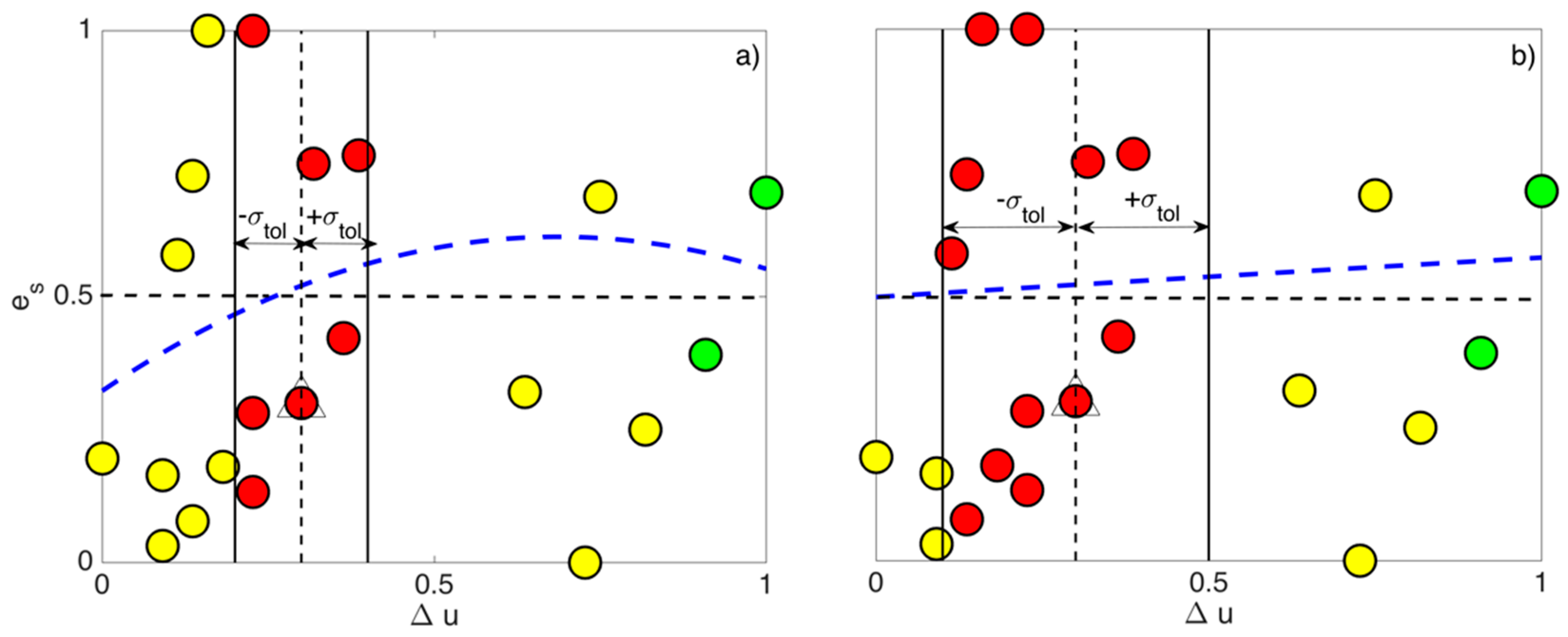
2.2.1. The 1D DUPID Controller

To ensure the quality of the regression data, this approach partitions the set $\mathbb{U}$ composed of $N_{pp}$ points pairs $(\Delta u^{\left(j\right)},e_s^{\left(j\right)}$) into two subsets with respect to the last gathered point $(\Delta u^{\left(k\right)},e_s^{\left(k\right)}$) (red point fitted within triangle). The effect of data segmentation carried out by the 1D DUPID is shown in Figure 4.

The last point obtained in the regression set will be addressed as the center point. The first subset, i.e., the vicinity set $U_v$, is comprised of all the points encompassed in $\pm {\sigma }_{tol}$ distance of the center point, measured on the $\Delta u$ axis (red points). The point selection in this version of the algorithm is carried out solely with respect to the coordinate $\Delta u$ (hence its “one-dimensional” nature). The second subset, the outer set $U_o$, contains the remaining points that are further from the center point $\Delta u^{\left(k\right)}\pm {\sigma }_{tol}$ (yellow and green points). The approach of segmenting the regression data is carried out to ensure the constructed model compromises between local precision on one hand and robustness on the other hand. The local precision of the model is guaranteed by the points found in the vicinity set $U_v$ whereas the robustness is established by the points found in the outer set $U_o$. In this paper, the robustness of the fit is guaranteed by considering two anchor points (the green points) from the outer set. The anchor points are regarded as points whose distance with respect to $\Delta u^{\left(k\right)}$ is greatest. After the regression set $U_r=\left\{U_v,U_o\right\}$ is constructed, the model parameters $p=\left\{A,B,C\right\}$ are calculated from the optimization problem defined as:

$$\underset{p}{\min }{\displaystyle \sum }_{r=1}^{n_r}{\left(e_s^{\left(r\right)}-E_M\left(\Delta u^{\left(r\right)},p\right)\right)}^2,$$

(5)

where, $n_r$ is the number of points in the regression set, $\Delta u^{\left(r\right)}$ are the points found in $U_r$, the set of the past control error values is defined as $e_s=\left\{e_s^{\left(1\right)}, \dots , e_s^{(n_r)}\right\}$, and $E_M\left(\Delta u^{\left(r\right)},p\right)$ describes the quadratic model given with Equation (3). Next, $\Delta u^{\left(j+1\right)}$ is calculated as:

$$\Delta u^{\left(j+1\right)}=\underset{\Delta u_i}{\mathrm{argmin}}\left|\Delta u_i-\Delta u^{\left(k\right)}\right|,$$

(6)

where $\Delta u_i$ represent, the roots of Equation (3):

$$\Delta u_i=\left\{\Delta u_i| E_M=0\right\}.$$

(7)

However, there might be a situation where the constructed fit does not intersect with the zero error axis. In such occasions $\Delta u^{\left(j+1\right)}$ is calculated by differentiation of the constructed model:

$$\Delta u^{\left(j+1\right)}=-\frac{B}{2A}.$$

(8)

Afterwards, $\Delta u^{\left(j+1\right)}$ is applied to the plant, and as a new error point $e_s^{\left(j+1\right)}$ is obtained, the array of past $N_{pp}$ points is moved with center at ($\Delta u^{\left(j+1\right)},e_s^{\left(j+1\right)})$ and the procedure for calculation of the next incremental value is repeated.

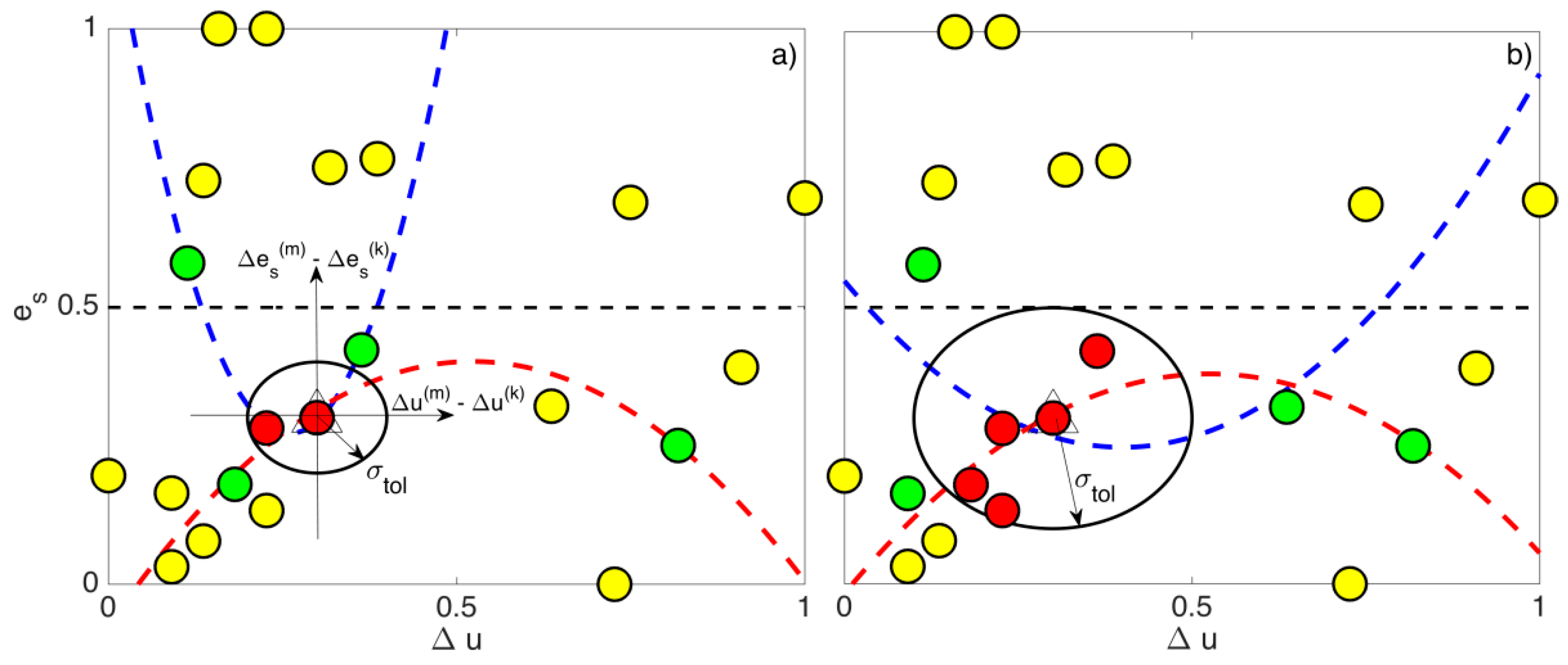
2.2.2. The 2D DUPID Controller

The process of selection of regression data in 2D DUPID is given in Figure 5. The 2D DUPID uses two coordinates, $\Delta u$ and $e_s$, in the process of points selection. This is carried out by calculating the Euclidian distances of each of the $N_{pp}-1$ points with respect to the center point $\left(\Delta u^{\left(k\right)},e_s^{\left(k\right)}\right)$. As a result, a local coordinate system around the last point is placed (see Figure 5a):

$$D_m=\sqrt{{\left(\Delta u^{\left(m\right)}-\Delta u^{\left(k\right)}\right)}^2 +{\left(e_s^{\left(m\right)}-e_s^{\left(k\right)}\right)}^2};m=1,\dots ,N_{pp}-1.$$

(9)

At first, the vicinity set $U_v$ consists of all the points encompassed by the circle centered at $\left(\Delta u^{\left(k\right)},e_s^{\left(k\right)}\right)$ with radius ${\sigma }_{tol}$ (red points):

$${\left(\Delta u^{\left(m\right)}-\Delta u^{\left(k\right)}\right)}^2+{\left(e_s^{\left(m\right)}-e_s^{\left(k\right)}\right)}^2\le {\left({\sigma }_{tol}\right)}^2.$$

(10)

The outer set $U_o$ includes the points with distance greater than ${\sigma }_{tol}$. (green and yellow points). Those points are additionally sorted based on the angles they form with the center point. If the number of points present in the outer set is larger than four, then the algorithm proceeds with the segmentation of the outer set until a point is found in each local quadrant with the smallest distance $D_m$ (green points). If the number of points is less than four, then all points are considered for regression. Finally, if the number of points found is exactly four, then two outer subsets are formed, each comprised of two points. The first outer subset $U_o^1$ contains the points found in the local quadrants 1 and 2, and the second outer subset $U_o^2$ contains the points found in the local quadrants 3 and 4. The major downside of this approach is that it may suffer in terms of time and computer resources needed for those four points to be found. The underlying idea of splitting the outer set into two subsets is to ensure that the data are fitted by two quadratic models (red and blue dashed lines), where at least one of them intersects with the zero error axis (black dashed line).

The subsets constructed from the outer set are defined as: $U_o^1=\left\{\Delta u_o^{\left(1\right)},\Delta u_o^{\left(2\right)}\right\}$ and $U_o^2=\left\{\Delta u_o^{\left(3\right)},\Delta u_o^{\left(4\right)}\right\}$. The values contained in both regression sets $U_r^1=\left\{U_v,U_o^1\right\}$ and $U_r^2=\left\{U_v,U_o^2\right\}$ are related to the entries found in the error sets, $e_s^{\left(1\right)\left(r\right)}$ and $e_s^{\left(2\right)\left(r\right)}$, respectively. The model parameters, $p^{\left(1\right)}=\left\{A_1,B_1,C_1\right\}$ and $p^{\left(2\right)}=\left\{A_2,B_2,C_2\right\}$ for both models are calculated from two optimizations problems, each defined as:

$$\underset{p^{\left(i\right)}}{\min }{\displaystyle \sum }_{r=1}^{n_r}{\left(e_s^{\left(i\right)\left(r\right)}-E_M^{\left(i\right)}\left(\Delta u^{\left(i\right)\left(r\right)},p^{\left(i\right)}\right)\right)}^2, i=1,2;$$

(11)

where $n_r$ is the number of points in the regression set, $\Delta u^{\left(i\right)\left(r\right)}$ are the points found in $U_r^{\left(i\right)}$, $E_M^1\left(\Delta u^{\left(1\right)\left(r\right)},p^{\left(1\right)}\right)$ is the quadratic model constructed from the $\left(U_r^1,e_s^{\left(1\right)\left(r\right)}\right)$ set, and $E_M^2\left(\Delta u^{\left(2\right)\left(r\right)},p^{\left(2\right)}\right)$ is the model constructed based on the $\left(U_r^2,e_s^{\left(2\right)\left(r\right)}\right)$ set. Next, $\Delta u^{\left(j+1\right)}$ is calculated in a similar fashion as given with Equation (6), but the number of roots can vary depending on, whether the constructed models intersect with the zero error value axis or not. As a result, there might be three cases:

• Both constructed models intersect with the zero error axis. The total number of roots, in this case, is $i=4$;
• Just one of the constructed models intersects with the zero error axis. The total number of roots, in this case, is $i=2$;
• None of the constructed models intersects with the zero error value. Consequently, the next incremental value $\Delta u^{\left(j+1\right)}$ is chosen as the minimum value of the model that predicts the smallest error.

After $\Delta u^{\left(j+1\right)}$ is calculated, it is applied to the plant and a new error point $e_s^{\left(j+1\right)}$ is attained. The procedure of calculating the next incremental value is repeated by moving the coordinate system at ($\Delta u^{\left(j+1\right)},e_s^{\left(j+1\right)})$.

3. Results

3.1. Case Study

In this paper, as a benchmark plant model for the controllers the highly nonlinear continuous stirred tank reactor (CSTR) system, Figure 6, with varying parameters is considered.

The model equations were taken from [20]. The CSTR system is a second-order control system which is modelled by the Equations (12) and (13). In spite of the simplicity of this model, it is well known by its strong nonlinear dynamics which is often manifested by: strong dependence of particular parameters, steady-state multiplicity, limit cycle etc. [23].

$$\frac{dT}{dt}=\frac{q}{V}\left(T_f-T\right)+\frac{\Delta H}{\rho C_p}{k}_0{C}_A{e}^{-\frac{E}{RT}}+\frac{h{A}_{ta}}{V\rho C_p}\left(T_c-T\right),$$

(12)

$$\frac{d{C}_A}{dt}=\frac{q}{V}\left(C_{Af}-C_A\right)-k_0{C}_A{e}^{-\frac{E}{RT}}.$$

(13)

The parameters of the model are defined as: $q$—Volumetric flow-rate; $V$—Volume of the CSTR; $\rho$—Density of the mixture; $C_p$—Heat capacity; $\Delta H$—Heat of the reaction; $E$—Activation energy; $R$—Universal gas constant; $k_0$—Pre-exponential factor; $h$—Overall heat transfer coefficient; $A_{ta}$—Heat transfer area; $T_f$—Feed fluid temperature; $C_{Af}$—Feed concentration of reactant A; $T_c$—Temperature of the cooling jacket; $C_A$—Concentration of reactant A; $T$—Temperature in the CSTR. The nominal values assumed for the plant parameters are given in

Table 1. The considered nominal values for the parameters of the CSTR plant.

Parameter	Value	Parameter	Value
$q$	$100 \mathrm{L}/\min$	$h{A}_{ta}$	$5·{10}^4 \mathrm{J}/\min \mathrm{K}$
$V$	$100\mathrm{L}$	$T_f$	$350 \mathrm{K}$
$\rho$	$1000 \mathrm{g}/\mathrm{L}$	$C_{Af}$	$0.5 \mathrm{mol}/\mathrm{L}$
$C_p$	$0.239 \mathrm{J}/\mathrm{g}\mathrm{K}$	$T_c\left(0\right)$	$300 \mathrm{K}$
$\Delta H$	$5·{10}^4 \mathrm{J}/\mathrm{mol}$	$C_A\left(0\right)$	$\approx 0.46 \mathrm{mol}/\mathrm{L}$
$E/R$	$8750 \mathrm{K}$	$T\left(0\right)$	$\approx 318.9 \mathrm{K}$
$k_0$	$7.2·{10}^{10}1/\min$	$[T_{c, min}, T_{c, max}]$	[250, 350] K

. The manipulated variable is assumed to be the cooling jacket fluid temperature $T_c$, which is operated in the interval $\left[250, 350\right] \mathrm{K}$, and the reactor temperature $T$ is assumed to be the controlled variable, and the only measured state.

For relevant comparison between the discussed control algorithms, it is assumed that the heat transfer coefficient h and the feed fluid temperature $T_f$ change over time. These changes are realistic in practice as they often occur as a result of material deposition (fouling film) on the heat transfer surfaces, over the period of the plant operation. The process of fouling film development on the heat transfer surfaces is a slow and gradual process, which as a consequence adds resistance to the flow of heat. There are two types of fouling film build-up: asymptotic and linear. In the former, the resistance due to the fouling film increases very quickly at the beginning of the operation and becomes asymptotic to a steady-state value at the end. In the latter, the fouling film develops linearly over the entire period of plant operation [24].

Here, linear deposit contamination was assumed, and the parameters $h$ and $T_f$ were assumed to be subjected to linear change. The heat transfer coefficient $h$ is replaced in Equation (12) by $h_d$, which is defined as:

$$h_d={\varphi }_h\left(t\right)h=\left(1-{\alpha }_{h}t\right)h,$$

(14)

where $t$ is time, $h$ is the value of the heat transfer coefficient, $h_d$ is the scaled version of the heat transfer coefficient, ${\varphi }_h\left(t\right)\in \left(0,1\right)$ is the fouling coefficient (the scaling coefficient), and ${\alpha }_h$ is the fouling constant. The feed fluid temperature $T_f$ was assumed to be constant for a certain period of time, before changing into a ramp function in a negative direction. To broaden the discussion further, it was assumed that $T_f$ changes as ramp function in positive direction also:

$$T_f=\{\begin{array}{c}{T}_{fconst};1\le i<lb\\ \pm T_d\frac{i-lb}{i_{max}-lb}+T_{fconst}; lb\le i\le i_{max}\end{array},$$

(15)

where $T_{fconst}$ is the initial value of the feed temperature, $lb$ defines the interval of simulation time steps $i$ while $T_f$ is kept constant, $T_d$ defines how much $T_f$ changes in the positive or negative direction, and $i_{max}$ is the maximal number of simulation time steps. The model equations are numerically solved in MATLAB by the function ode23t with simulation time step $T_i=0.1 \min$.

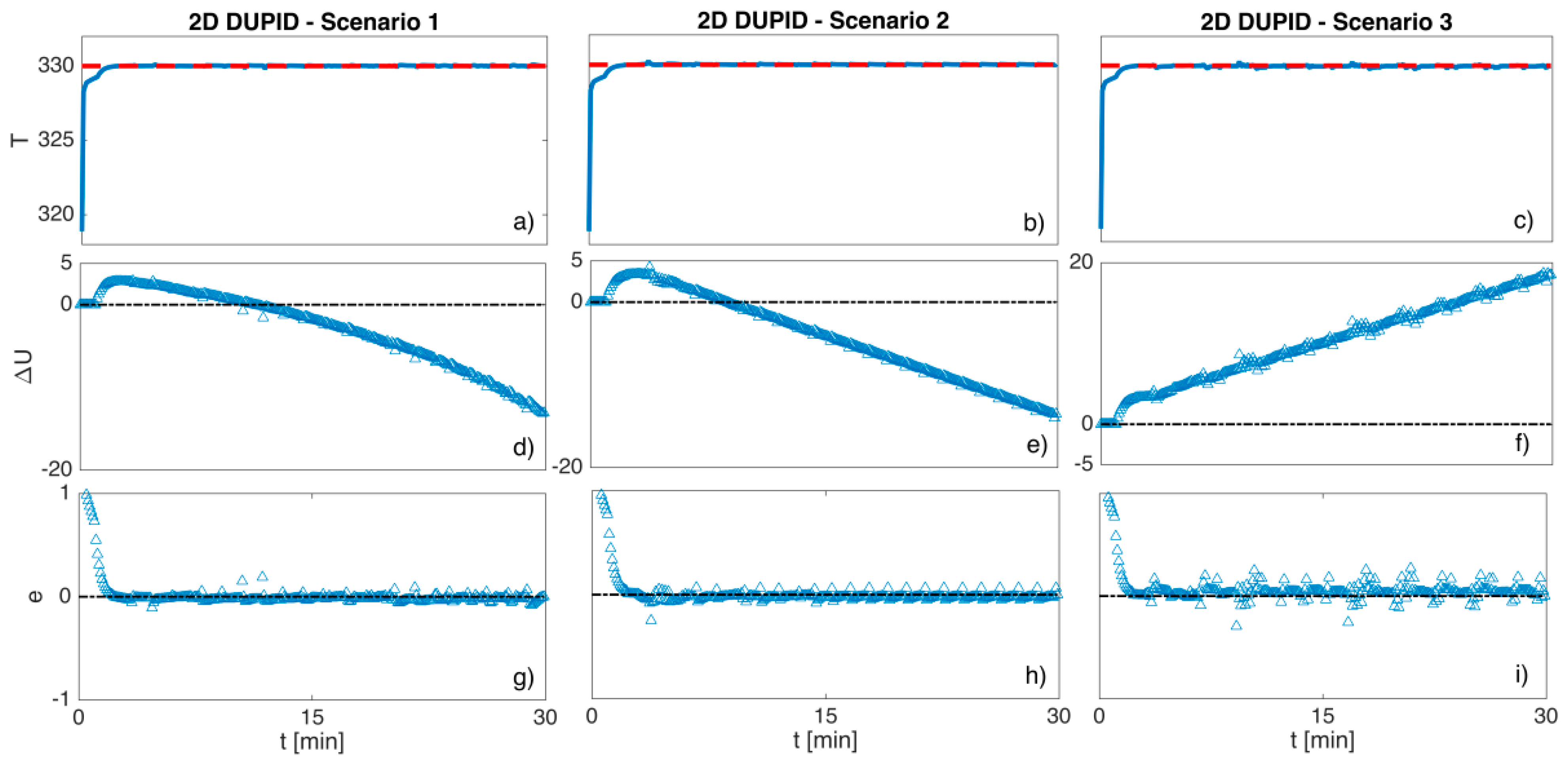
3.2. Simulation Results and Discussion

In this section, the control performances of the 1D and 2D DUPID controllers are compared against a benchmark PID controller. The benchmark PID controller is tuned by trial and error, as it is carried out in numerous industrial plants. To support this fact, in [25] the authors are referring to a statistic indicating that 30% of the PID controllers in the industry operate in manual mode and require continuous fine-tuning and supervising by the process technologist. Additionally, in [26], it is reported that 25% of the PID applications use coefficients that are pre-set by the manufacturer with no update of their values with respect to the particular process. Therefore, to showcase a realistic scenario, the parameters of the PID controller are tuned by trial and error assuming non-varying plant parameters. The PID controller parameters were assumed to be constant over the plant operation and they were selected so that the plant output achieves smooth transient response and zero steady-state error, without breaching the bounds of the interval of admissible control values. As a quantifying measure for the performance assessment of the controllers, the Integral of Absolute Error (IAE) metric is used (Equation (16)).

$$IAE=\frac{1}{i_{max}}{\displaystyle \sum }_{i=1}^{i_{max}}\left|e^{\left(i\right)}\right|.$$

(16)

For the sake of relevant comparison, three scenarios were addressed when the controllers were applied to control the CSTR system. These three scenarios are defined as follows:

• In the first scenario (Scenario 1), it is assumed that the heat transfer coefficient linearly drops to 50% of its initial value. Therefore, the value of ${\alpha }_h$ was assumed to be 0.0167.
• In the second scenario (Scenario 2), it is assumed that the feed temperature $T_f$ linearly increases for $T_d=+40 K$ of its initial value, $T_{fconst}=350 K$. The value of $lb$ is $30$.
• In the third scenario (Scenario 3), it is assumed that the feed temperature $T_f$ linearly drops for $T_d=-40 K$ of its initial value $T_{fconst}=350 K.$ The value of $lb$ is $30$.

The PID parameters were tuned to be $K_p=4.5, K_i=3.31$ and $K_d=0.01$. All DUPID parameters are pre-set and are constant in all scenarios. The DUPID parameters in both versions are assumed to be constant in all scenarios, $N_{pp}=12$ and ${\sigma }_{tol}=0.1$. The simplest guideline for tuning these two parameters would be to select the value of the first parameter ($N_{pp})$ to be at least three times larger (we used here four times larger number) than the minimum needed points for establishing the model given with Equation (3), while selecting the value of 0.1 for the latter parameter $\left({\sigma }_{tol}\right)$ will be suitable in most of the cases. Regarding the rest of the DUPID parameters, the $k_{ss}$ value is set to be 1 and $DV$ is given as:

$$DV=\{\begin{array}{c}D{V}^{\left(i\right)}=10;i \in \left[1,10\right]\\ D{V}^{\left(i\right)}=1; i \in \left[11,i_{max}\right]\end{array}.$$

(17)

The SM calculates the first incremental value after ten simulation time steps (one minute), whereas the other incremental values are calculated in each simulation time step. The idea behind the calculation of the first incremental value after ten simulation time steps is to start adding bias after the plant is settled in the steady-state. Adding bias during the transient state can provoke an unwanted overshoot in the plant response, or in the extreme case, it can destabilize the plant. The possible downside of calculating the other incremental values in each simulation time steps is having the added computational time burden. On the other hand, this can be justified by achieving a smaller IAE value and a better overall control performance.

In a real case scenario, the number of time steps needed to pass for the SM to start calculating the incremental value will be determined based on the plant itself, and on the experience of the process technician (the operator) on how much time is needed for the plant output to settle in steady-state. However, to omit the possible subjective human decision, in future modifications of the DUPID algorithm the moment of the first incremental value calculation should be determined automatically by accounting for the proximity of the PV with respect to the SP over time.

The simulation time step is assumed to be $T_i=0.1$ min. In the first ten simulation time steps (until minute 1) the value of $\Delta u$ is kept on zero since the first calculated incremental value by SM is carried out at the tenth time step. The termination criterion was defined with respect to the maximum permitted time steps $i_{max}=300$. The total time of the plant operation is $i_{max}·T_i=30$ min.

In Figure 7, the resulting plant response under PID control in all three scenarios is given. It is indicative that the error area increases over time in all scenarios, (d), (e) and (f). This is a consequence of the changing plant parameters over time. Since the PID controller coefficients are kept constant the controller is unable to adapt to the change in plant operating conditions and is therefore unable to steer the controlled variable ($T$) to the set point.

The 1D and 2D DUPID controllers proved to be more agile in detecting and countering the effects caused by the time-varying parameters. From the Figure 8d–f and Figure 9d–f, it can be seen that the DUPID anticipates the change in plant parameters and pushes the PID control value in the right direction to compensate for its stationary coefficients.

The control performance of each controller was quantified by the IAE metric,

Table 2. Table (a) contains the average time needed for calculating the incremental value by each DUPID controller in the considered scenarios (Scen.). In the last column of this table, the relative differences (RD) are given. In table (b), the integral of absolute error (IAE) values obtained by the controllers in each scenario are given, and in the last table, (c), the relative differences of the obtained IAE values by the controllers are given.

(a)	Time in sec.
Scen.	1D	2D	RD
1	0.0436	0.1007	0.5670
2	0.0497	0.1105	0.5502
3	0.0514	0.1070	0.5196
(b)	IAE values
Scen.	1D	2D	PID
1	0.1002	0.1005	0.2529
2	0.1066	0.1084	0.2781
3	0.1097	0.1337	0.2960
(c)	RD values
Scen.	1D/2D	1D/PID	2D/PID
1	0.0030	0.6038	0.6026
2	0.0166	0.6167	0.6102
3	0.1795	0.6294	0.5483
Avg.	0.0664	0.6166	0.5870

b. The relative differences (The relative difference is calculated as $d_r=\left|x-y\right|/\max \left(\left|x\right|,\left|y\right|\right)$) of the obtained IAE values, Table 2c, were calculated for each scenario. On average, the 1D DUPID and 2D DUPID controllers achieved improvement over PID control performance of around $62\%$ and 59%, respectively. The direct comparison between 1D and 2D DUPID controllers showed that 1D DUPID is performing slightly better, on average of around $7\%$ (Table 2c) first column). Moreover, we compared 1D and 2D DUPID in terms of how much time is needed on average for each controller to calculate the incremental value in each scenario, Table 1. From the values of the calculated relative differences, it is clear that 2D DUPID needs around twice as much time on average to produce the next incremental value compared to the 1D DUPID. This is an expected result having in mind that the 2D DUPID has an added computational burden which comes from its design to search for a point in each of the four quadrants of the local coordinate system placed around the centre point. Overall, the two controllers 1D and 2D DUPID showed that they can steer the controlled variable toward the set point with satisfactory precision.

4. Conclusions

In this paper, we discussed an improved version of the PID controller, the Dynamically Updated PID controller. The DUPID controller is constructed based on the assumption that the parameters in the plant vary with time in a smooth and gradual fashion. Its objective is to track the variation of the parameters and to intervene in the PID control value to reduce the increasing control error, which is a direct consequence of their variation. This controller resides on the paradigm of using recent history error data to construct a quadratic model that models the error caused by the varying parameters. This model is then exploited for the iterative calculation of a sequence of incremental values, which are applied directly to the PID control value, without changing the controller parameters, for the purpose of lessening the effect caused by the varying parameters in plant’s output.

The control performance of the DUPID controller is dependent on the precision of the quadratic model. To ensure the quadratic model describes the data well, the regression data used for its construction must fulfil certain criteria. In this regard, we discussed two versions of DUPID, the 1D and 2D DUPID. These versions differ in the approach of how the data are selected before the model coefficients are determined: the 1D DUPID uses only one coordinate in the process of regression data selection, whereas the 2D DUPID uses two coordinates for data selection.

We compared the control performances of the conventional parallel-form PID controller and the DUPID controllers (1D and 2D DUPID). Both controllers were applied to the CSTR system with varying parameters. We observed the control performance of the controllers in three scenarios which were derived from the assumption that the parameters $h$ and $T_f$ vary linearly over the time the plant is controlled. The results showed that the DUPID controller was capable of reducing the control error to a satisfactory level, whereas the PID control performance dropped with time. Finally, we performed a direct comparison between 1D and 2D DUPID controllers, and the results showed that their control performances do not differ by much.

To illustrate that the DUPID controller has the potential of broader use, different than the one discussed here, a meaningful control scenario is pinpointed in the Supplementary Materials. Namely, the DUPID controller is used to attribute the problem of the poorly tuned integral term in the PID controller. In this scenario, it was assumed that the integral term ($K_i$) of the PID controller is seriously mistuned and the set-point is changing as a ramp function. The results indicated that the DUPID controller accomplished set-point tracking with satisfactory steady-state error, and therefore it was able to make up for the mistuned integral term. To show that the improvement is genuine, we simulated the plant for 10 different uniformly distributed values of $K_i$ drawn from the interval $\left[0.01,1\right]$. For all the realizations of $K_i$ the DUPID showed superior performance with respect to the mistuned PID controller.

There are few open questions that will be addressed in the future versions of the DUPID controller:

First of all, to prove that the DUPID controller is multifaceted, it should be tested on the same plant discussed here, but when the concentration of the reactant A ($C_{Af}$) or the volumetric flow rate ($q$) are subject to change. Moreover, it will be tested on more complex high-order nonlinear processes of practical importance. In the next modifications, the DUPID algorithm will be adapted to be able also to detect and tackle step changes in the plant parameters.

In addition, a trust-region based on covariance analysis around the centre point will be included. The importance of the trust-region will be twofold; it will constrain the algorithm to calculate an incremental value in the direction of poor level data spread and, at the same time, it will define bounds of the validity of the model.

Lastly, after the aforementioned improvements are implemented, the DUPID controller will be tested based on its ability to average out the noise that is omnipresent in real plants.

Furthermore, one should note that in this paper, the focal point was set on discussing the hands-on implementation of the DUPID controller without elaborating on the stability margins of the proposed algorithm. However, the topic of stability is a significant issue in control engineering, so further investigations will be conducted on establishing a formal mathematical proof of the asymptotical stability of the plant around a given set-point when DUPID is used as controller. This discussion is motivated by the result reported in [27], where the authors proved that for CSTRs that are isothermal and asymptotically stable, a classical PI compensator can yield to global asymptotic stabilization about a prescribed operating point [23].

References

1. Åström, K.J.; Hägglund, T.; Astrom, K.J. Advanced PID Control. vol. 461. ISA-The Instrumentation, Systems, and Automation Society Research Triangle. 2006. Available online: https://www.researchgate.net/publication/3207690_Advanced_PID_Control_-_Book_Review (accessed on 19 January 2021).
2. Rotach, V.Y. Teoriya Avtomaticheskogo Upravleniya: Uchebnik dlya VUZov (Automated Control Theory: University Textbook), 5th ed.; MEI Publishing House: Moscow, Russia, 2008. [Google Scholar]
3. Fahmy, R.A.; Badr, R.I.; Rahman, F.A. Adaptive PID Controller Using RLS for SISO Stable and Unstable Systems. Adv. Power Electron. 2014, 2014, 1–5. [Google Scholar] [CrossRef]
4. Ziegler, J.G.; Nichols, N.B. Optimum Settings for Automatic Controllers. J. Dyn. Syst. Meas. Control. 1993, 115, 220–222. [Google Scholar] [CrossRef]
5. Haykin, S.S. Adaptive Filter Theory; Pearson Education India: Chennai, India, 2008. [Google Scholar]
6. Åström, K.J.; Wittenmark, B. Adaptive Control; Courier Corporation: North Chelmsford, MA, USA, 2013. [Google Scholar]
7. Tian, B.; Su, H.; Chu, J. An optimal self-tuning PID controller considering parameter estimation uncertainty. In Proceedings of the 3rd World Congress on Intelligent Control and Automation (Cat. No.00EX393), Hefei, China, 26 June–2 July 2000; pp. 3107–3111. [Google Scholar] [CrossRef]
8. Martínez, J.I.O.; Paz Ramos, M.; Garibo, S.; Luna-Ortega, C. PI controller with dynamic gains calculation to comply with time specs in presence of parametric disturbances. In Proceedings of the 6th International Conference Electrical Engineering, Computing Science and Automatic Control, Toluca, Mexico, 10–13 November 2009. [Google Scholar]
9. Xiao, S.; Li, Y.; Liu, J. A model reference adaptive PID control for electromagnetic actuated micro-positioning stage. In Proceedings of the 2012 IEEE International Conference on Automation Science and Engineering (CASE), Seoul, Korea, 20–24 August 2012; pp. 97–102. Available online: http://citeseerx.ist.psu.edu/viewdoc/download?doi=10.1.1.721.2583&rep=rep1&type=pdf (accessed on 19 January 2021).
10. Petersen, I.R.; Tempo, R. Robust control of uncertain systems: Classical results and recent developments. Automatica 2014, 50, 1315–1335. [Google Scholar] [CrossRef]
11. Vilanova, R.; Alfaro, V.M.; Arrieta, O. Robustness in PID Control. In PID Control in the Third Millennium; Springer: London, UK, 2012; pp. 113–145. [Google Scholar]
12. Morari, M.; Zafiriou, E. Robust Process Control. 1989. Available online: https://cse.sc.edu/~gatzke/cache/morari-zafiriou-PI-chapters1-3.pdf (accessed on 19 January 2021).
13. Lee, Y.; Park, S.; Lee, M.; Brosilow, C. PID controller tuning for desired closed-loop responses for SI/SO systems. AIChE J. 1998, 44, 106–115. [Google Scholar] [CrossRef]
14. Ge, M.; Chiu, M.-S.; Wang, Q.-G. Robust PID controller design via LMI approach. J. Process. Control 2002, 12, 3–13. [Google Scholar] [CrossRef]
15. Garpinger, O.; Hägglund, T. A Software Tool for Robust PID Design. IFAC Proc. Vol. 2008, 41, 6416–6421. [Google Scholar] [CrossRef] [Green Version]
16. Mercader, P.; Astrom, K.J.; Banos, A.; Hagglund, T. Robust PID Design Based on QFT and Convex–Concave Optimization. IEEE Trans. Control. Syst. Technol. 2016, 25, 441–452. [Google Scholar] [CrossRef]
17. Stavrov, D.; Nadzinski, G.; Stojanovski, G.; Deskovski, S. Performance analysis of DUPID control over CSTR sys-tem with varying parameters. In Proceedings of the 14th International Conference ETAI, Struga, Macedonia, 20–22 September 2018; pp. 2545–4889. [Google Scholar]
18. Wenzel, S.; Gao, W.; Engell, S. Handling Disturbances in Modifier Adaptation with Quadratic Approximation. The research leading to these results was funded by the ERC Ad-vanced Investigator Grant MOBOCON under the grant agreement No. 291458. IFAC-PapersOnLine 2015, 48, 132–137. [Google Scholar] [CrossRef]
19. Wenzel, S.; Paulen, R.; Engell, S. Quadratic Approximation in Price-Based Coordination of Constrained Systems-of-Systems. Focapo/cpc. 2017. Available online: http://folk.ntnu.no/skoge/prost/proceedings/focapo-cpc-2017/FOCAPO-CPC%202017%20Contributed%20Papers/92_CPC_Contributed.pdf (accessed on 19 January 2021).
20. Seborg, D.E.; Mellichamp, D.A.; Edgar, T.F.; Doyle, F.J., III. Process Dynamics and Control; John Wiley & Sons: Hoboken, NJ, USA, 2010. [Google Scholar]
21. O’Dwyer, A. Handbook of PI and PID Controller Tuning Rules; Imperial College Press: London, UK, 2009. [Google Scholar]
22. Brunton, S.L.; Kutz, J.N. Data-Driven Science and Engineering: Machine Learning, Dynamical Systems, and Control, 1st ed.; Cambridge University Press: Cambridge, UK, 2019. [Google Scholar]
23. Alvarez, J.; Alvarez-Ramirez, J. Linear PI control of batch exothermic reactors with temperature measurement. Int. J. Robust Nonlinear Control 2006, 16, 113–131. [Google Scholar] [CrossRef]
24. Nikravesh, M.; Farell, A.E.; Stanford, T.G. Control of nonisothermal CSTR with time varying parameters via dy-namic neural network control (DNNC). Chem. Eng. J. 2000, 76, 1–16. [Google Scholar] [CrossRef]
25. Bucz, Š.; Kozáková, A. Advanced methods of PID controller tuning for specified performance. PID Control Ind. Process 2018, 73–119. Available online: https://www.intechopen.com/books/pid-control-for-industrial-processes/advanced-methods-of-pid-controller-tuning-for-specified-performance (accessed on 19 January 2021).
26. Yu, C.-C. Autotuning of PID Controllers: A Relay Feedback Approach; Springer Science & Business Media: Berlin, Germany, 2006. [Google Scholar]
27. Alvarez-Ramirez, J. Global stabilization of chemical reactors with classical PI control. Int. J. Robust Nonlinear Control IFAC Affil. J. 2001, 11, 735–747. [Google Scholar] [CrossRef]
Figure 1. PID (Proportional–Integral–Derivative) control loop structure.
Algorithms 14 00031 g001
Figure 2. Dynamically updated PID (DUPID) control loop structure.
Algorithms 14 00031 g002
Figure 3. The flow chart diagram of the DUPID controller.
Algorithms 14 00031 g003
Figure 4. The effects of using of 1D DUPID algorithm to select adequate data for model construction for different values of σ t o l : (a) σ t o l = 0.1 and (b) σ t o l = 0.2 . The blue dashed lines in (a,b) are the obtained quadratic fits. The last point fed to the algorithm is marked with a triangle. The collected data used for testing consist of 20 random integer points drawn on the interval [ 0 , 50 ] for Δ u and [ 70 , 70 ] for e s . The data are normalized before it is fed to the algorithm. The black dashed line is zero error axis mapped in the normalized search space.
Algorithms 14 00031 g004
Figure 5. The effects of using of 2D DUPID algorithm to select adequate data for model construction for different values of σ t o l : (a) σ t o l = 0.1 and (b) σ t o l = 0.2 . The blue and red dashed lines in (a,b) are the obtained quadratic fits. The last point fed to the algorithm is marked with a triangle. The collected data used for testing consist of 20 random integer points drawn on the interval [0, 50] for Δ u and [−70, 70] for e s . The data are normalized before it is fed to the algorithm. The black dashed line is zero error axis mapped in the normalized search space.
Algorithms 14 00031 g005
Figure 6. Graphical representation of the Continuous Stirred Tank Reactor (CSTR) system.
Algorithms 14 00031 g006
Figure 7. The plant response under PID control in all three scenarios. The figure is structured in two rows of three pictures, in the first row (ac) show the plant output (blue line) and the set point (red dashed line); in the second row (df) show the resultant control error (blue markers) is plotted against the zero error line (black dashed line).
Algorithms 14 00031 g007
Figure 8. The plant response under 1D DUPID control in all three scenarios. The figure is structured in three rows of three pictures, in the first row (ac) the plant output (blue line) and the set point (red dashed line) are plotted; in the second row (df) the incremental value is given (blue markers); in the third row (gi) the resultant control error (blue markers) is plotted against the zero error line (black dashed line).
Algorithms 14 00031 g008
Figure 9. The plant response under 2D DUPID control in all three scenarios. The figure is structured in three rows of three pictures; in the first row (ac) the plant output (blue line) and the set point (red dashed line); in the second row (df) the incremental value is given (blue markers); in the third row (gi) the resultant control error is given (blue markers) and it is plotted against the zero error line (black dashed line).
Algorithms 14 00031 g009