3. Description of the Algorithm
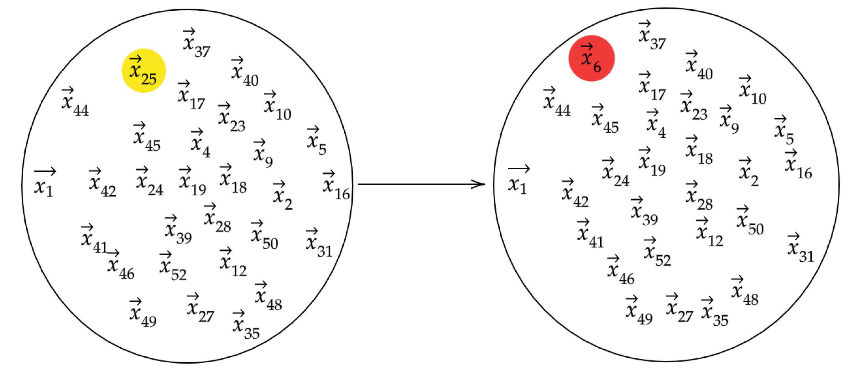
Our algorithm is motivated by the intuition that if we take a data set of vectors that represent typical behavior and one of the vectors were replaced with an anomalous observation, the topology of the data set would be significantly altered. The topology of the set is understood by computing persistence diagrams of randomly chosen subsets
. When we modify a bag
by randomly replacing one of its vectors with
we denote the resulting modified bag by
.
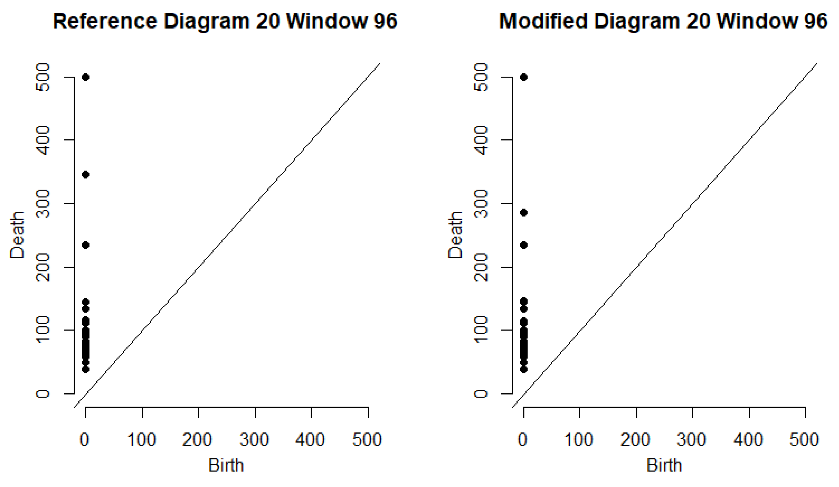
Figure 2 depicts the data points in the reference and modified bags. We then let
D and
denote the persistence diagrams for vectors in
and
, respectively.
Figure 3 depicts the persistence diagrams for the reference and modified bags for a specfic data point.
The bottleneck distance quantifies how much the topology of a set has changed. We say there is evidence that
is anomalous if
is relatively large compared to the values in
. There are some undesirable cases that may occur due to the random sampling used to form
. It may be that the observations contained in
do not adequately represent the entire data set, or if the reference bag contains an anomaly, we might replace an anomaly with a non-anomalous vector when forming the modified bag. To mitigate issues such as these, the algorithm uses multiple bags of the same size. We select hyperparameters
and repeat
N times the process of randomly choosing
S vectors to form
. This creates a collection of reference bags
. For each of the
N bags, we form
m distinct modified bags
by randomly choosing
and replacing it with
. We calculate the summary statistics mean, median, and standard deviation for the bottleneck distances, and choose a function
that identifies anomalies from the summary statistics. The entire algorithm is presented in Algorithm 1.
| Algorithm 1: Anomaly Detection using Persistence Diagrams of Random Subsamples |
 |
The summary statistics of the bottleneck distances can be used in various ways depending on the application. In our application to traffic data, we set thresholds for each summary statistic based on training data. Thus, we set thresholds for the three summary statistics, and we defined if and only if and .
In addition to those previously mentioned, we may also encounter the issue when the modified bag
is formed by replacing the same vector
. This would make an anomaly look much less anomalous based on our bottleneck distance measurement. Fortunately, if
N is chosen to be sufficiently large, then the effect can be very small since the summary statistics converge in probability. Let us formalize the probability distribution here. The sample space consists of ordered pairs
We place the uniform distribution on and denote this by .
Theorem 1. Let , , and be denote the mean, standard deviation, and median respectively of bottleneck distance associated with as computed in Algorithm 1. Then there exist , and such that as , and for all , Proof. Define the random variable
on
by
We have that
are i.i.d. random variables. Since
and there are no infinite points in
,
is bounded. The three limits are consequences of the Weak Law of Large Numbers, which requires a sequence of i.i.d. random variables with finite expectation. In particular, let
and
. Since the
are i.i.d. with finite mean
, by the Weak Law of Large Numbers,
as
. To prove the second limit, we start by writing
Since
are i.i.d with
, it follows from the Weak Law of Large Numbers that
as
N tends to infinity. Since we have established
as
, it follows that
as
N tends to infinity. Adding up the terms in (
1), this means
in probability. For the third equation, first define
For any
, we have
. We can define
if
, and
otherwise. It follows that
. Since
is the sample median of
, it follows that
Since
, we apply the Weak Law of Large Numbers to
to see that
. Similarly, we have
, Thus, if we instead define
if
, we have
. Much like what we had in (
2), we find
Since , we again have from the Weak Law of Large Numbers applied to that . □
Remark 2. Since we are sampling from a discrete probability distribution, it is not guaranteed that the distribution producing the has a true median. Hence we must settle for convergence of the sample median to some interval. In the case where there exists η such that , then and the sample median converges in probability to η. We define the sample median the usual way where if , the sample median would be if N is odd or if N is even.
Remark 3. We note that the values guaranteed in Theorem 1 are data dependent, and that for the purposes of Theorem 1 as well as Algorithm 1, the data are fixed.
4. Results
In this section, we present our contribution to the ATD challenge problem through the application of our method on traffic data collected from major highways in the Sacramento area. The problem was divided into two phases–depending on whether the location information of the sensors was provided–where each phase consisted of a training and testing data set. The objective of each phase of the challenge problem was to predict the time and location of hand-selected traffic incidents in the testing data using the training data which had very few labeled incidents. The data was collected as a count of cars that passed a given sensor during each 5-min interval throughout the 2017 calendar year. An example of this can be seen in
Table 1.
The training sets included details on certain incidents reported during the year that include the nearest sensor, the timestamp, and the duration of each incident. In each data set there are a few instances in which a particular sensor was not operating so that there are no counts reported during those five-minute intervals.
Table 2 contains additional information on the data sets that were provided.
To apply the algorithm to the volumetric data, we considered the embedding of the data in as sequences of 12 consecutive 5-min counts from a sensor. This means each vector represents 1 hour’s worth of counts. We index each vector by a 3-tuple . We use p to denote the sensor ID from which the counts were collected. We let , where t denotes the starting time of the five-minute window corresponding to the first of the 12 counts and indicates the day of the week with corresponding to Sunday, corresponding to Monday, etc. We let denote the week in which these counts were collected. (We note that in 2017, there were 53 Sundays, and so for , .) The vectors were then sorted by sensor, starting time, and day of week, meaning the set of all vectors was partitioned into smaller data sets of 52 vectors. We let denote the collection of count vectors from sensor p collected at the time (hour and day of the week) corresponding to . For two different starting times from the same weekday, say and , it is possible that the components of vectors in overlap with those of vectors in . For example, if 8:00 AM, and 8:05 AM, then the vectors in are nearly the same vectors as in , but the entries are shifted left by one component and the final entry is the count from 9:00–9:05 AM. Since there are 288 five-minute intervals throughout the day and we required 12 consecutive counts to form each vector, there are 277 possible vectors of counts each day.
After sorting the vectors, we applied Algorithm 1 to each collection of counts with and . Thus, each vector in , was assigned 30 bottleneck distances. For each time window , we recorded the mean, median, and standard deviation of these bottleneck distances which we denote by , , and , respectively.
As in [
53], we expected different periods of the day to exhibit different behavior. Therefore, after obtaining the summary statistics from Algorithm 1, our vectors were classified again according to three factors: day of week, sensor, and time of day. Time of day had 5 levels based on the time of the vector’s first count. The levels were
Early Morning, Morning, Mid Day, Evening, and
Late Evening, and they corresponded to one-hour windows with start times in the ranges:
The windows were ranked by each of their summary statistics within their classification. These rankings were given in the form of a percentile and used as anomaly scores.
We expected that traffic patterns throughout the year should be fairly consistent given a particular sensor, day of the week, and period of the day; however, it is possible that traffic behavior could be unusual for an entire day due to a holiday, road construction, or a weather event. Then, according to this window classification, it cannot be readily ascertained if a particular window with a relatively large mean bottleneck distance is due to something acute, such as a traffic incident, or to something predictable, like Labor Day or a major sporting event. We took this into account by reclassifying the windows by sensor, time of day, and day of the year. We then ranked the windows a second time within each of these treatment groups. Each window was assigned 6 percentile scores, based on three different summary statistics each ranked two different ways.
We describe our procedure using an example from the Phase 2-Train data. To measure the likelihood that there was an incident occurring near sensor
on Monday, 6 February 2017, during the window from 7:55 AM to 8:55 AM, we set
. We apply our algorithm to
. See
Figure 3 for an example of the persistence diagrams related to this particular timestamp. If an incident occurred on February 6th, the sixth Monday of 2017 in the time window classification, we would expect that
would be large compared to the rest of the collection
. When this is done, we find that
, which is the second largest of the 52 average bottleneck distances in
. Even though this was not the largest average bottleneck distance observed for this sensor, day of week, and time of day, it did rank above the mid-98th percentile among all
Mid Day windows according to average bottleneck distance for
on a Monday. Similarly,
ranked above the 96th percentile and of standard deviations of bottleneck distance, and
ranked just above the 99th percentile of median bottleneck distances observed from
Mid Day, Monday windows at sensor
S314402. If we consider this window among only the observations from
Mid Day on February 6th at sensor
, then
ranks just above the mid-89th percentile,
ranks above the mid-90th percentile, and
is at least tied as the highest ranking sample median of its class.
After the six rankings are determined for each window in our data set, we are ready to apply selection criteria to determine which windows overlapped with traffic incidents. The selection consists of six thresholds for the six rankings. The thresholds are determined by the rankings of windows near the starting times of the labeled incidents in the training data using the procedure outlined below:
Identify all windows starting within 30 min of the timestamp of a reported incident at the same sensor where the incident was located.
For each of the 6 types of rankings, identify a minimum ranking needed to include at least one window corresponding to each labeled incident. If all 6 minimum rankings seem too small, the minimum ranking to include one window from all but one incident could be used instead.
Set the first threshold, as the largest of the six minimums.
Identify which of the windows found in step 1 satisfy the threshold of
For each of the 5 types of rankings that were not used to determine , identify the minimum ranking met by all the windows identified in step 4.
Set the other 5 thresholds, according to the 5 minimums identified in step 5.
Once the thresholds are set, we classify all windows that have all six rankings each above their respective thresholds as incidents. In the rest of this section, we present the results when this procedure is applied to each of the four data sets. We present the rankings of windows near each incident in the data sets and the thresholds we determined from training data sets. In each phase, we use the thresholds determined by the training data to classify the windows in the corresponding testing data. We measure the performance of these predictions using precision, recall and an F-score.
Remark 4. Our performance evaluation using Algorithm 1 exclude any incidents detected on Sundays since the training data did not include any reported incidents on Sunday.
To provide some comparison, we also apply a standard normal deviates (SND) algorithm to detect incidents in the phase-1 data. The SND algorithm detects an incident in the
kth 5-min time window if the count for that window,
, satisfies
We let
and
respectively denote the mean count and standard deviation of counts from the same treatment group and
denotes some threshold that applies across all treatment groups. In this case, a treatment group is made up of all counts belonging to the same sensor, on the same day of week, at the same time of day. For example, in Phase-1, there were 52 counts taken at sensor
, on Monday mornings at 8:00 AM,
. We can compute the mean and standard deviation of this treatment group,
For a better description of the SND algorithm and its application to incident detection see [
11], where incident detection was performed using vehicle velocity rather than traffic flow. The threshold
was determined using the Phase 1-Train data by computing the deviates for each window occurring during a labeled incident. For each of the 15 incidents, we computed the 85th percentile of the counts that took place during the incident. We chose
to be the second smallest of the 15 percentiles we computed. Thus, for the phase 1 data, we found
, meaning any 5-min window where the count exceeded 1.06 standard deviations from the mean was detected as an incident.
4.1. Data without Sensor Locations
In the Phase 1-Train data set, we were able to find windows near the incidents that had very large average bottleneck distances. When sorted by sensor, day of week, and time of day, all of the 15 labeled incidents overlapped with a one-hour window starting within half an hour of some window that was ranked in the 85th percentile. When sorting these sensors further by day of year, the start time of six of the incidents fell within half an hour of the window with the highest average bottleneck distance in their category.
Table 3 and
Table 4 present the percentile scores of the incidents in the Phase 1-Train dataset.
Table 5 contains the 6 thresholds determined using the rankings of windows near the labeled incidents. The quality of the fit is given in
Table 6; as a comparison, the quality of fit using the standard normal derivates is given in
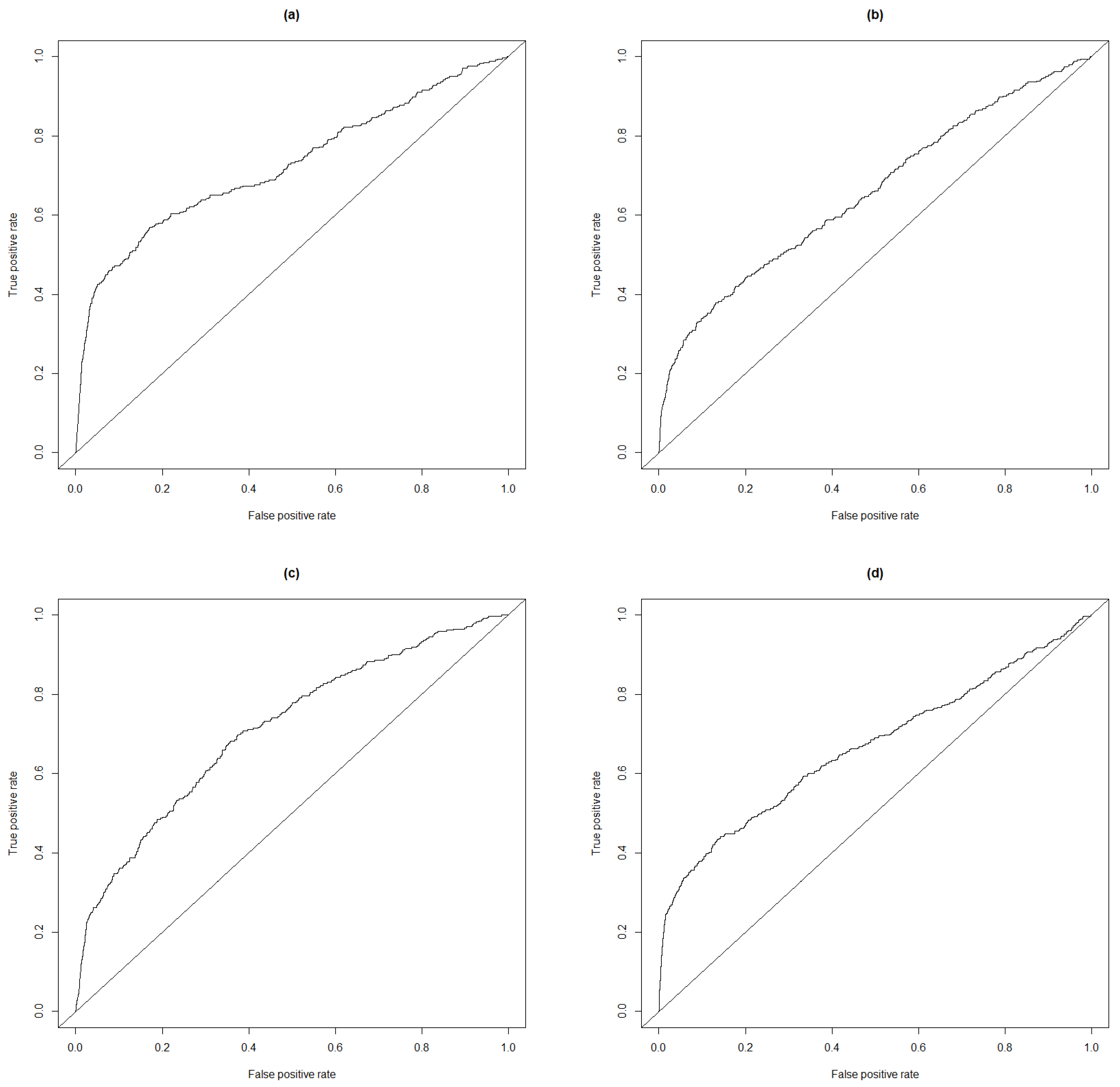
Table 7. To better describe the quality of the anomaly scores, we provide the receiver operating characteristic (ROC) curve based on the three rankings in
Figure 4. We also provide the ROC curve based on the standard normal deviates.
Of course, these performance scores say very little about the method since the thresholds were determined using the incidents in the data set. Rather, we apply the thresholds in
Table 5 to classify the Phase 1-Test data.
Table 8 has the performance scores from this experiment, whereas
Table 9 has the performance for the standard normal deviates on this dataset.
4.2. Data with Sensor Locations
In Phase 2 we were given the locations of the sensors in terms of latitude and longitude.
Table 10 and
Table 11 display the nine incidents reported in Phase 2-Train and the largest percentile recorded for each summary statistic in windows starting within half an hour of the starting time of each incident at the sensor where the incident was reported.
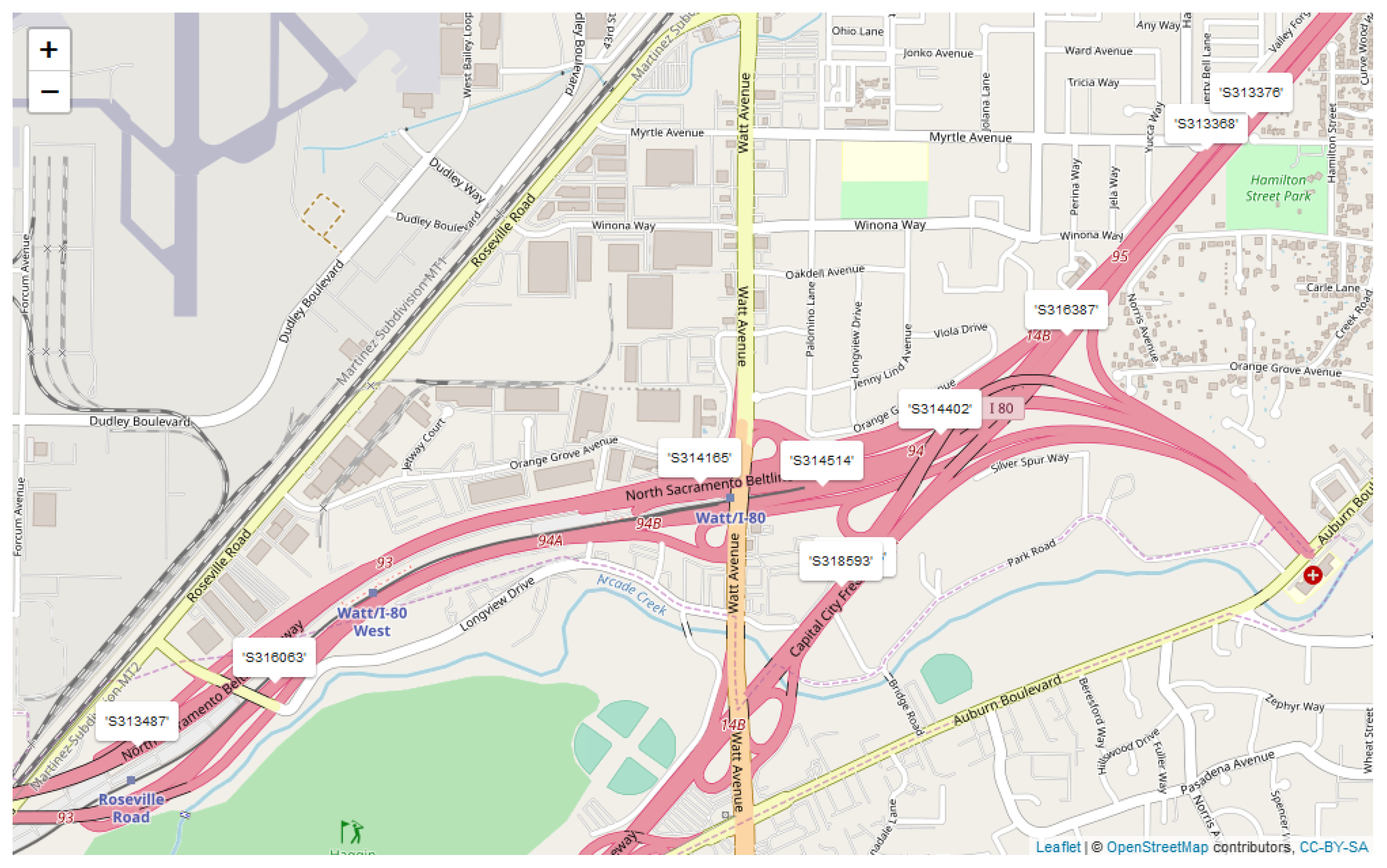
Depending on the severity of the incident, it is possible that a traffic incident occurring near one sensor will cause some abnormal behavior in the counts of the adjacent sensors. For example, in the network of sensors used in the Phase 2-Train data, traffic flows directly from
to
. A map of all the sensor locations in this data set is provided in
Figure 1. If one of the lanes is obstructed near
it is likely to slow down traffic between the two sensors. This might cause the counts from
to look fairly large when compared to
. On the other hand, if a motorist was able to anticipate this problem in the traffic a mile ahead, they might deviate their route before even passing
. If enough cars did this, there would be a lower count at the first sensor, but the count at
might still be higher because of all the unfortunate cars that got caught between the sensors at the time of the incident. In either scenario, we would expect some unusual behavior when we compare the counts of both sensors together. Not knowing if the difference should be large or small, we apply the random bagging algorithm to the sequence of differences between the counts, with the intuition that if an incident occurred during a particular hour, especially one with lots of traffic, the mean bottleneck distance for that time window would also be large. We refer to the summary statistics obtained from this procedure as adjacency statistics. In
Table 12 and
Table 13 we provide the highest rankings near the reported incidents based on the adjacency statistics.
The most noticeable difference made by the adjacency statistics can be observed by the percentile of the July incident when windows are sorted by sensor, day of year, and time of day. The highest any window near that time ranks by average bottleneck distance of raw counts is in the 66th percentile of Mid Day counts for that day, but if we consider the differences in counts between the two adjacent sensors, we find the highest ranking Mid Day window for July 24th starts within half an hour of the July incident.
With the addition of the adjacency statistics, we had 12 percentiles to consider for each window.
Table 14 presents the 12 thresholds determined from the incidents in the data for Phase 2-Train. The quality of the fit is given in
Table 15. We only report the performance statistics for sensors
and
since those were the only sensors in the data set where incidents were labeled.
As in Phase 1, we use the thresholds learned from the training data to classify the windows in the Phase 2-Test data. In this data set, there were 8 sensors. The 8 sensors formed 8 pairs of adjacent sensors, meaning we were able to compute adjacency scores for the windows on every sensor. In
Table 16 we present the performance scores for this classification. The data for Phase 2-Test was very different from any of the other data sets. There were 1409 incidents with an average duration of 42 min. Surprisingly, no true incidents were reported at sensor
.


