Abstract
In order to improve the efficiency of transportation networks, it is critical to forecast traffic congestion. Large-scale traffic congestion data have become available and accessible, yet they need to be properly represented in order to avoid overfitting, reduce the requirements of computational resources, and be utilized effectively by various methodologies and models. Inspired by pooling operations in deep learning, we propose a representation framework for traffic congestion data in urban road traffic networks. This framework consists of grid-based partition of urban road traffic networks and a pooling operation to reduce multiple values into an aggregated one. We also propose using a pooling operation to calculate the maximum value in each grid (MAV). Raw snapshots of traffic congestion maps are transformed and represented as a series of matrices which are used as inputs to a spatiotemporal congestion prediction network (STCN) to evaluate the effectiveness of representation when predicting traffic congestion. STCN combines convolutional neural networks (CNNs) and long short-term memory neural network (LSTMs) for their spatiotemporal capability. CNNs can extract spatial features and dependencies of traffic congestion between roads, and LSTMs can learn their temporal evolution patterns and correlations. An empirical experiment on an urban road traffic network shows that when incorporated into our proposed representation framework, MAV outperforms other pooling operations in the effectiveness of the representation of traffic congestion data for traffic congestion prediction, and that the framework is cost-efficient in terms of computational resources.
1. Introduction
Cars have become the preferred means of transportation for more and more people due to the rapid development of urbanization and improvement of people’s living standards. The huge number of cars has become very challenging in terms of the efficient operation of urban road traffic networks and causes traffic congestion. Road traffic congestion in many cities around the world is very serious, especially in metropolitan cities [1]. There have been a lot of research on the prediction of urban road traffic congestion and traffic management [2,3,4,5]. Understanding the congestion patterns of an entire road network rather than a single road or several roads in an area is important. Prediction of traffic congestion helps people choose better routes and helps traffic administration departments manage and operate road networks more effectively and more efficiently [6,7].
With the development and improvement of intelligent transportation systems, traffic data has become more and more accessible due to factors such as the deployment of road sensors and probes, free availability of online map services, and widespread popularization of GPS services and equipment such as smart phones. Similar to other industries, the field of transportation has entered the era of big data. One of the challenges proposed by the large amount of traffic-related data is how to represent large-scale traffic data and apply various models to utilize these data.
In recent years, researchers have utilized various types of urban traffic flow data as inputs to different kinds of models for the prediction of traffic flow variables such as speed, volume, density and demand [8]. Two methods dominate the research of traffic prediction: parametric and nonparametric methods [5,9]. Parametric methods require a model’s structure and parameters to be determined in advance according to theoretical or physical assumptions [9]. Auto regressive integrated moving average (ARIMA) is a typical parametric method. This method builds a model based on historical time series data to predict future values. ARIMA and other ARIMA-based models, such as seasonal ARIMA (SARIMA) models [10,11,12], KARIMA models [13], ARIMAX models [14], and CTM-SARIMA models [15], have been used to predict traffic flow variables such as congestion and volumes [13,16].
Compared with parametric methods, nonparametric methods are flexible because their structure and parameters are not fixed. The support vector machine (SVM) approach is based on statistical learning theory and is very popular when making prediction because it can transform low-dimensional nonlinear data to high-dimensional space through a kernel function [17]. SVMs together with their variants, such as SVR, seasonal SVM, PSO-SVM, and online-SVM, have been utilized for traffic flow prediction [18,19,20,21]. Another typical nonparametric method is neural networks. Neural networks are widely used in almost all fields including traffic flow prediction. Neural networks can model complex nonlinear relationships and have an excellent performance in processing multidimensional data [22]. In recent years, deep neural networks have been involved in traffic flow prediction, such as deep belief networks (DBN) [23] and deep neural networks [24]. Although these neural network-based methods are suitable for small traffic networks or networks with a small number of roads, they cannot take advantage of spatial correlations among different roads and temporal dependencies of traffic flow variables.
On the other hand, for neural network models, especially deep neural network models, oversized input data make models use too many computing resources, such as GPU memory, and also cause overfitting [25]. Additionally, such input data increase the training and prediction time of models, which restricts the application of neural network models. In order to alleviate such problems, there are methods in the existing literature which are used to represent traffic flow data about road networks. These methods aim to reduce the sizes of traffic flow data and lower the demand of computation resources while at the same time preserving the spatial structures of traffic networks as much as possible.
At present, in the related literature regarding the prediction of traffic flow variables of urban road traffic networks, one commonly used method to represent traffic flow data for an urban road traffic network is to first segment that network into consecutive equally sized grids, and then apply a certain pooling operation, such as addition or arithmetic mean, to values of traffic flow variables in each grid. For example, Hu et al. segmented a road network of Beijing into grids when predicting traffic speed using floating car data from taxis, and then they calculated the average speed for these grids [26]. When predicting the traffic flow of Beijing and New York City, Zhang et al. divided each city into grids in longitude and latitude directions, and counted the number of vehicles entering and leaving each grid within a certain time interval [27]. Yu et al. segmented a local road network in Beijing when predicting speed in that area, and used the average speed of all road segments covered by each grid as that grid’s speed [5]. Xu et al. divided the urban area of Beijing into grids when predicting speed on roads in that area, and calculated each grid’s average speed in the same way as Yu et al. for every 30 min [28]. Duan et al. segmented an urban area of Xi’an into 16 × 16 grids and summed the number of trips from a certain origin to a certain destination when predicting the number of such trips [29]. Zhang et al. divided a metropolitan freeway transportation network in Seattle into grids and calculated the average congestion level for each grid when predicting traffic congestion in that area [30]. However, these operations are often selected without further consideration, and specifically, there has rarely been an evaluation of their impacts regarding the prediction of traffic flow variables.
Although this existing scheme has facilitated the prediction of traffic flow variables such as traffic volume, speed, congestion, and demand, until recently there has been little in-depth research on how to properly represent traffic congestion data for an urban road network in order to retain its spatial structure as much as possible and to predict traffic congestion on its road segments. Compared with the prediction of other traffic flow variables, prediction of traffic congestion in an urban traffic network is much more intuitive for and practically significant to both travelers and traffic management departments. For travelers, traffic congestion prediction helps one to choose better travel routes and reduce pollution associated with emissions from vehicles. For traffic management, it can improve operational efficiency by controlling and coordinating urban road traffic networks. Therefore, we propose a representation framework for traffic congestion data in urban road networks. This framework aims to reduce the size of large-scale traffic congestion data in order to lower the requirements of computing resources for deep learning models. Moreover, it does not damage the performance of models used to predict traffic congestion.
The contributions of the paper can be summarized as follows:
- We develop an effective and cost-efficient representation framework for traffic congestion data of urban road networks. This framework combines grid-based partition of urban road traffic networks and a pooling function to reduce the size of traffic congestion data, while at the same time still retaining the spatial structure of road networks on a courser scale;
- We construct a model based on convolutional neural networks and long short-term memory neural networks to learn both spatiotemporal correlations and dependencies of traffic congestion between road segments and predict traffic congestion in road networks;
- The effectiveness and efficiency of our proposed representation framework is demonstrated by extensive experiments on a typical urban road traffic network.
The remainder of this paper is organized as follows. Section 2 presents a detailed account of our proposed framework and pooling operation. Section 3 describes extensive experiments on a dataset of traffic congestion for an urban road traffic network, which verify the effectiveness, efficiency, and feasibility of the proposed approach. Finally, Section 4 provides some conclusions.
2. The Proposed Approach
In this section we first propose our framework for the representation of traffic congestion data of a road network. Our proposed representation framework consists of two steps. The first step segments original traffic congestion matrices into equally sized grids. The second step reduces all values in each grid using a pooling operation into a single value which will replace all values in that grid, and thus, the size of original traffic congestion matrices is reduced in a way similar to image down-sampling [31]. These two steps are described in Section 2.1 and Section 2.2. Then, we construct a deep learning model based on CNNs and LSTMs to evaluate the effectiveness of the proposed representation framework.
We use raw snapshots, as shown in Figure 1a, of traffic congestion maps captured from online map service providers as a raw data source for traffic congestion data. As can be seen in Figure 1a, roads are marked with different colors for different congestion levels which provide useful traffic congestion data, yet there are also background and other nonroad elements which are not needed and thus need to be removed. In order to keep only roads marked with congestion information, an image mask is derived from a special kind of raw snapshots of traffic congestion maps for the same area. Such special raw snapshots are special in that all roads in them are marked with the color for being smooth, which is green, as used by almost all online map service providers. They are widely available late at night when there are few vehicles running on roads. As an example, Figure 2a shows such a special raw snapshot captured at 02:54, 30 March 2019. With help of image processing algorithms, green pixels for smooth roads are converted to 1 while all other pixels were converted to 0. Thus, an image mask was obtained as shown in Figure 2b. After background removal using image masks for road networks, these raw snapshots are transformed into images like Figure 1b, which only keep a road network whose road segments are marked with congestion levels using different colors, for example green, yellow, red, and dark red. Then, each of these network-only images is converted into a matrix, with each pixel inside turned into a normalized value in according to color of that pixel’s congestion level. Although the derived properties of traffic flow, such as the congestion intensity [32] and congestion index [33], in the existing literature are defined on wider ranges of values, such value ranges are inappropriate as direct inputs to deep learning models for the prediction of traffic congestion, because without being normalized they cause a problem known as internal covariate shift [34]. Such matrices form a set of original traffic congestion matrices. As discussed in Section 1, these original traffic congestion matrices need to be reduced because of the often limited availability of computing resources and to prevent overfitting.
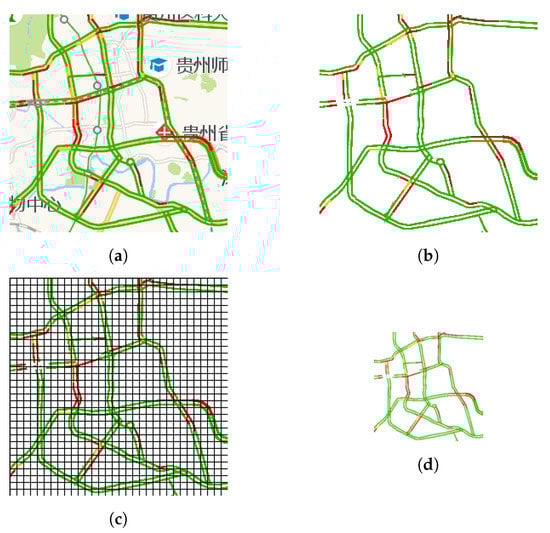
Figure 1.
Congestion maps of an urban area traffic network in Guiyang, Guizhou, China. (a) A raw snapshot of the traffic network’s congestion map. (b) Only the road network marked with congestion levels is retrained after removing the background and other elements. (c) An original congestion matrix visualized as a network-only image is partitioned into grids. (d) A down-sampled traffic congestion matrix rendered as a map.
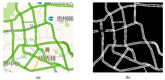
Figure 2.
Transformation from a special raw snapshot to a derived image mask based on it. (a) A special raw snapshot captured at late night. (b) A derived image mask.
2.1. Grid-Based Partition of Congestion Data
Let be an original traffic congestion matrix with M rows and N columns representing traffic congestion levels for a road network at time t as shown below:
where each element of is a numerical value representing one traffic congestion level for a corresponding pixel of a raw traffic congestion map snapshot captured at time t.
After grid-based partition of using a grid size of , now is divided into grids. As an intuitive visual illustration, Figure 1c shows this segmentation process applied to a network-only image corresponding to . For a grid located at (i, j) where , and , denotes the set of values for congestion levels as represented by all pixels in that grid at time t.
2.2. Reduction of Grid Values
Each of these grids of are reduced into a single value through a pooling operation, so that is converted into a compressed traffic congestion matrix with R rows and C columns, as shown below:
where an element of will be calculated by a pooling function applied upon a set which contains all values in a grid index by of .
Through this process of grid-based partition and reduction, each element of is a derived value representing one corresponding grid of .Thus, is now down-sampled and compressed into by a ratio of , yet the relative spatial relationships between roads are mostly kept, as shown in Figure 1d.
Pooling operations used by the reduction process above are requisite to our proposed approach because the effectiveness of grid-based representation of road network traffic congestion data is determined by such operations, which act as a kind of feature extraction filter. We propose a pooling function which retrieves the maximum of all values (MAV) in a grid of , which is rarely used when representing traffic congestion data. MAV is described by Equation (1):
2.3. Prediction Model
Convolutional neural networks (CNNs) use convolution filters to extract local and global features through sliding windows, and can learn spatial correlations of traffic flow variables nearby or in entire cities [22,27,35,36,37]. Long short-term memory neural networks (LSTM) were proposed by Hochreiter and Schmidhuber in 1997 [38]. They can learn temporal relationships and dependencies from time series data and have been applied to short-term traffic prediction [5,39,40,41]. Deep learning models combining CNNs and LSTMs are widely used in the literature regarding traffic flow prediction and can capture both the spatial correlations and temporal dependencies of traffic flow variables on road networks [5,36,42,43,44].
On the basis of the popularity and performance of models combining CNNs and LSTMs in the existing literature, we propose a spatiotemporal traffic congestion network (STCN) based on CNNs and LSTMs to evaluate the effectiveness of our proposed representation framework for traffic congestion data. An overview of STCN’s architecture is shown in Figure 3. STCN contains three main components. The first component consists of four CNNs and is used to learn spatial features and their correlations to traffic congestion between roads in a road network. The second consists of two LSTMs and is used to mine temporal dependencies across a series of historical traffic congestion data. Finally, the third has a full connection layer and a reshape operation to construct predicted traffic congestion in that road network.
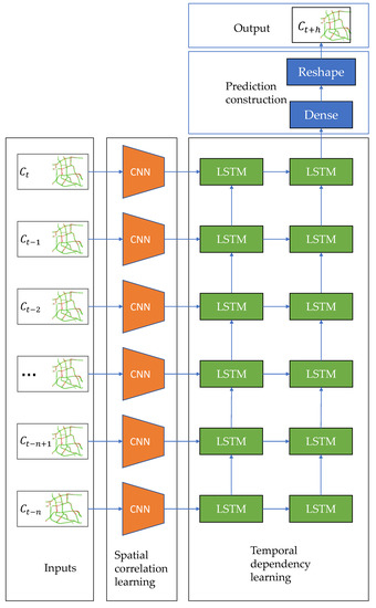
Figure 3.
Architecture of the prediction model.
The first component takes a sequence of matrices in the form of ordered chronologically as its input. The spatial features and correlations extracted by the first component are used as inputs to the second component. The output by the second component is processed by the third to predict traffic congestion levels and construct a traffic congestion map as output.
Additionally, a max-pooling layer is used after each convolution layer to select representative features, and a batch-normalization layer to overcome internal covariate shift. A dropout layer is inserted before the full connection layer to prevent overfitting.
3. Experiments
3.1. Dataset
Originating from various traffic detectors [45] or powered by online map services such as Google Maps [46], real-time traffic condition maps of transportation networks are regularly archived in the form of snapshots by transportation administration departments 24 h a day, 7 days a week, and are provided online [47,48]. In order to build a dataset of traffic congestion data, we first create an initial data source in this work by complying with procedures used by these transportation administration departments. Figure 1a is an example of a raw snapshot of a traffic congestion map for an urban area in Guiyang, Guizhou province, China, which was one of top 10 most congested major cities in China in 2019 [49]. Each raw snapshot for this area is 256 pixels wide and 256 pixels high and mainly covers urban arterial roads. Such snapshots are retrieved at a scale of 1:50,000 every 10 min during morning rush hours between 07:00 and 10:00 from 1 January 2019 to 30 September 2019 through a free API provided by an online map service provider AutoNavi [50]. Requests to that API sometimes fail and cause missing data, which are left blank as is in this paper. These snapshots form an initial data source of traffic congestion data.
After their background and other nonroad elements have been removed as described in Section 2, raw snapshots from our initial data source are transformed into network-only images. Then, we use these network-only images containing road segments marked with congestion levels to build a dataset for traffic congestion research. The congestion level given by the color of each pixel inside images like Figure 1b is linearly converted to a normalized value based on its color (transparent, green, yellow, red, or dark red) to form an original traffic congestion matrix [30]. Specifically, transparent pixels are converted to 0.0, green ones to 0.25, yellow ones to 0.5, red ones to 0.75, and dark red one to 1.0, because traffic congestion levels are categorized by the online service provider based on the calculated linear travel time index. Gray pixels in a network-only image such as Figure 1b indicate road segments inaccessible or with missing data and are treated as transparent ones. After conversion, the size of original traffic congestion matrices is .
3.2. Comparative Methods and Metric
Pooling operations applied to values in each grid of an original traffic congestion matrix determine the effectiveness of our proposed representation framework, as discussed in Section 2.1. We compare our proposed MAV pooling operation with three others used in the existing literature:
- The nearest neighbor value (NNV), as defined by Equation (2), is based on a common image resampling algorithm [51]. In our experiment, this operation returns the value in the upper left corner of a grid [52];
- The average of the maximum and minimum values (AMM) which is inspired by weighted median filter [53,54]. In our experiment, this operation returns the mean of the maximum value and minimum value in a grid, as defined by Equation (3);
- The nonzero average (ANZ) of the values in each grid used in the existing literature for the prediction of traffic flow variables such as speed or congestion [5,28], as defined by Equation (4).
3.3. Experiment Settings
Detailed descriptions of the architecture and parameter configuration of our STCN are shown in Table 1. It was implemented based on an open-source deep learning framework—Keras [55]. Experiments were run on a workstation with Ubuntu 18.04 installed. This experimental device had only one Nvidia GeForce RTX 2080 Ti graphics card which had 11,019 megabytes of GPU memory. The model was trained based on the optimizer RMSprop [56]. The learning rate was set to 0.001 and the decay parameter was set to 0.9. The batch size was dynamic because this model was trained and tested by day using back-testing, and thus missing data introduce different numbers of samples each day. The loss function was a customized weighted mean squared error (wMSE) defined in Equation (5), where stands for the penalty weight applied to different congestion levels because different congestion levels have different priorities. In addition, early stopping was used to prevent overfitting.

Table 1.
Architecture and parameter settings of CNN-LSTM.
STCN discussed in Section 2.3 was used to compare the accuracy of our proposed pooling method and the other three described above, which are essential to our proposed framework for the representation of road network traffic congestion data in a down-sampled and compressed way to predict traffic congestion.
Previous work determined an optimized time lag of 120 min for traffic prediction [57]. Therefore, for all pooling operations, 12 compressed traffic congestion matrices with an interval of 10 min during the past min arranged in chronological order were used as input to the STCN model. These input matrices were obtained after grid-based partition of the original traffic congestion matrices using a grid size of and the separate application of each of these four pooling operations. The reason for using a grid size of in our work is twofold. Firstly, it is inspired by its popular utilization in convolutional neural networks [25,58,59,60,61,62] and as a default pool size of pooling layers in deep learning frameworks such as Keras [55] and TensorFlow [63]. Secondly and more importantly, it can strike a balance between demand of computational resources and loss of traffic congestion information due to down-sampling [64,65]. The output of this model is a compressed congestion matrix at one of six short terms including typical prediction horizons of 10, 30, and 60 min as used in [5,30], and also 20, 40, and 50 min used in this paper. For all four pooling operations, the ground-truth matrices for the predicted output matrices were obtained after grid-based partition of corresponding original traffic congestion matrices using a grid size of and application of the NNV operation defined by Equation (2).
Instead of dividing the dataset into a training set and a test set by a certain fixed time point or using cross-validation, we used back-testing by day to compare the accuracy of each of the four pooling operations when incorporated into our proposed traffic congestion representation framework for traffic congestion prediction [30]. Traffic congestion levels in the morning rush hours between 07:00 and 10:00 on each of the 20 working days from 3 September 2019 to 30 September 2019 were tested. Traffic congestion data from the past 133 consecutive working days before each tested working day were used as training data.
We used mean absolute error (MAE), mean squared error (MSE), and roads-only mean absolute percentage error (roMAPE) defined respectively by Equations (6)–(8) as the accuracy metrics to evaluate the performance of the traffic congestion prediction when using different pooling operations inside our proposed representation framework in this paper. Because nonroad areas including background and other elements were converted to 0 in the original traffic congestion matrices, roMAPE only considers errors for which corresponds to an original traffic congestion matrix’s grid containing road segments marked with congestion levels. In these three equations, and respectively denote a ground-truth traffic congestion level and a predicted traffic congestion level at time t for an element indexed by () in a compressed traffic congestion matrix . In Equation (8), is the Iverson bracket which converts a logical proposition P to either 1 or 0 according to whether P is true or false.
3.4. Results
Table 2 and Figure 4 show the results of the accuracy metrics of our proposed representation framework incorporating each pooling operation, as evaluated by STCN. The metric values in Table 2 were rounded to four places and minimum values were marked with a bold typeface according to their original values before they were rounded.
Table 2.
Comparison of overall prediction metrics by different methods during 20 days with a prediction horizon of 10, 20, 30, 40, 50, and 60 min. Minimum metric values are marked with a bold typeface.
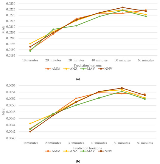
Figure 4.
Prediction errors for prediction horizons of 10, 20, 30, 40, 50, and 60 min. (a) Mean absolute error (MAE). (b) Mean squared error (MSE).
It can be seen that in terms of MSE, MAV achieved minimum average daily errors with 0.0050 for 30 min, 0.0052 for 40 min, and 0.0052 for 60 min. As for MAE, MAV performed better than the other three with 0.0189 for 10 min, 0.0211 for 30 min, 0.0219 for 40 min, 0.0219 for 60 min. With regard to roMAPE, MAV produced three minimum average daily errors with 5.6986 for 20 min, 5.8901 for 40 min, and 5.8229 for 50 min. Considering MSE, MAE, and roMAPE, in more than half of these six prediction horizons, MAV produced minimum errors when predicting traffic congestion levels. Additionally, Figure 2 illustrates the trends of MAE and MSE according to the four pooling operations along the prediction horizon. It can be observed that the prediction errors generally go upward, which might be caused by more uncertainties as the prediction horizon moves further into the future. However, MAV produces optimal overall prediction errors with a more stable trend than the others. Hence, it can be inferred that when used as a pooling operation, MAV together with our proposed framework can properly and effectively represent traffic congestion data for short-term traffic congestion prediction. The reason for MAV’s overall optimal performance might be twofold. Firstly, MAV always chooses the most serious congestion level in each grid, which is foremostly representative for real-world regions corresponding to these grids. Secondly, serious traffic congestion in one region is more likely to propagate to other ones. As for the other three pooling operations, NNV misses the most congested level in cases, while the other two reduce the significance and representativeness of the most congested level through averaging.
As an example of the prediction errors by day, details about the daily prediction performance in terms of MAE and MSE with a horizon of 40 min are shown in Figure 5. It can be seen that MAV has a smaller variation than ANZ, AMM, and NNV, which is confirmed by the standard deviation values shown in Table 3.

Figure 5.
Comparison of the daily prediction metrics with a prediction horizon of 40 min during 20 days, evaluated with back-testing. (a) Daily MAE. (b) Daily MSE.
Table 3.
Standard variations corresponding to Figure 5.
To evaluate requirement of computational resources, Table 4 lists the usage of GPU time and memory both by the original matrices and compressed ones derived using our proposed framework with MAV as the pooling reduction operation. When original traffic congestion matrices are used as input, STCN and these input data could not fit onto the one graphics card of our experiment device. Therefore, it had to be evaluated on another workstation with the same configuration as our experimental device, the difference being that it had two graphics cards of the same type described in Section 3.3. In addition, it was run with the help of a distributed deep learning framework—Horovod [66]. Metric values are reported as recorded on each experimental device. It can been seen the compressed matrices derived using our proposed representation framework combined with MAV save more than GPU time and use only a little more than of GPU memory when compared to the original matrices. Using a grid size of , original matrices are reduced by in size and thus our proposed representation framework is cost-efficient in terms of GPU time and memory.
Table 4.
Comparison of the required computing resources on original traffic congestion matrices and down-sampled ones using maximum of all values (MAV).
To compare the effectiveness of the original traffic congestion matrices (ORIGINAL) and the compressed ones derived using our proposed approach, Table 5 lists the average metric values of MAE and MSE across six prediction horizons. The metric values in Table 5 were rounded to four places and minimum values were marked with a bold typeface according to their original values before they were rounded. In terms of MSE, MAV commits smaller errors of 0.0047, 0.0050, 0.0052, respectively, for the prediction horizons of 20, 30, and 60 min. As for MAE, MAV performs better with error values of 0.0208, 0.0211, 0.0224, and 0.0219, respectively, for 20, 30, 50, 60 min into the future. It can be inferred that the compressed traffic congestion matrices derived using our proposed approach are at least as effective as the original ones, while at the same time are more efficient. This might be because the maximum value of a grid is characteristic of that gird. Particularly, when only a grid size of is used in our experiment, it is possible for the maximum value to well represent its grid with no loss of information.
Table 5.
Comparison of the effectiveness of original traffic congestion metrics and compressed ones derived using our proposed approach.
As an example of the prediction of traffic congestion levels using MAV as the pooling operation of our proposed representation framework and using STCN, Figure 6 shows several examples of both the ground truth congestion levels and the predicted ones on 25 September 2017, with a prediction horizon of 10 min. It can be seen that the predicted congestion maps are visually intuitive and recover congestion levels for most road segments in the network.
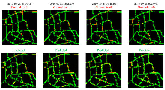
Figure 6.
Examples of ground-truth congestion maps (above) and predicted congestion maps (below) on 25 September 2019 with a prediction horizon of 10 min using MAV.
4. Conclusions
In this work, in order to reduce the usage of computational resources while at the same achieve optimal performance, we first propose a framework to represent urban road traffic network congestion levels. This was used to utilize historical records of traffic congestion data with a large size to predict future short-term traffic congestion levels. We captured raw snapshots of congestion maps for an urban road traffic network in Guiyang, Guizhou province, China. These snapshots were preprocessed and transformed into a dataset consisting of matrices representing traffic congestion levels at different times. To evaluate the effectiveness and cost-efficiency of our proposed MAV pooling operation, we compared its prediction performance with that of three other existing methods within our proposed representation framework. We also propose a deep learning neural network STCN for traffic congestion prediction, using it with the back-testing method. The results as regards our aforementioned dataset show that MAV achieves optimal overall performance and can effectively and cost-efficiently represent congestion levels in an urban road traffic network for short-term traffic congestion forecasting.
On the other hand, this study only focuses on the evaluation of the representation performance of traffic congestion levels using raw snapshots of a single urban area traffic network. In addition, MAV has a limited compression ratio because it depends on the grid-based partition of urban road traffic networks, restricting its scope in terms of applicable road networks. In future work, we will try to experiment with snapshots of congestion maps for different scales of road networks and look for other representation schemes to improve the compression ratio of urban road traffic networks, as to make it feasible to investigate congestion of traffic networks with larger scales.
Author Contributions
Conceptualization, S.Z. and X.L.; methodology, S.Z., Y.Y. and X.L.; software, S.Z.; validation, S.Z., X.L. and Y.Y.; formal analysis, S.Z.; investigation, S.Z.; resources, S.L.; data curation, S.Z.; writing—original draft preparation, S.Z., Y.Y. and X.L.; writing—review and editing, S.Z and Y.Y.; visualization, S.Z.; supervision, S.L.; project administration, S.L.; funding acquisition, S.L. All authors have read and agreed to the published version of the manuscript.
Funding
This research was funded by The National Natural Science Foundation of China under Grant No. 91746116 and 51741101, and Science and Technology Project of Guizhou Province under Grant Nos. [2018]5788, Talents [2015]4011 and [2016]5013, Collaborative Innovation [2015]02.
Conflicts of Interest
The authors declare no conflict of interest.
References
- Zheng, Y.; Li, Y.; Own, C.M.; Meng, Z.; Gao, M. Real-Time Predication and Navigation on Traffic Congestion Model with Equilibrium Markov Chain. Int. J. Distrib. Sens. Netw. 2018, 14. [Google Scholar] [CrossRef]
- Wen, F.; Zhang, G.; Sun, L.; Wang, X.; Xu, X. A Hybrid Temporal Association Rules Mining Method for Traffic Congestion Prediction. Comput. Ind. Eng. 2019, 130, 779–787. [Google Scholar] [CrossRef]
- Liu, Y.; Wu, H. Prediction of Road Traffic Congestion Based on Random Forest. In Proceedings of the 2017 10th International Symposium on Computational Intelligence and Design (ISCID), Hangzhou, China, 9–10 December 2017; Volume 2, pp. 361–364. [Google Scholar] [CrossRef]
- Chen, M.; Yu, X.; Liu, Y. PCNN: Deep Convolutional Networks for Short-Term Traffic Congestion Prediction. IEEE Trans. Intell. Transp. Syst. 2018, 19, 3550–3559. [Google Scholar] [CrossRef]
- Yu, H.; Wu, Z.; Wang, S.; Wang, Y.; Ma, X. Spatiotemporal Recurrent Convolutional Networks for Traffic Prediction in Transportation Networks. Sensors 2017, 27, 1501. [Google Scholar] [CrossRef] [PubMed]
- Zhang, J.; Wang, F.Y.; Wang, K.; Lin, W.H.; Xu, X.; Chen, C. Data-Driven Intelligent Transportation Systems: A Survey. IEEE Trans. Intell. Transp. Syst. 2011, 12, 1624–1639. [Google Scholar] [CrossRef]
- Park, J.; Li, D.; Murphey, Y.L.; Kristinsson, J.; McGee, R.; Kuang, M.; Phillips, T. Real Time Vehicle Speed Prediction Using a Neural Network Traffic Model. In Proceedings of the 2011 International Joint Conference on Neural Networks, San Jose, CA, USA, 31 July–5 August 2011; pp. 2991–2996. [Google Scholar]
- Lieu, H.; Gartner, N.; Messer, C.; Rathi, A. Traffic flow theory. Public Roads 1999, 62, 45–47. [Google Scholar]
- Van Lint, J.W.C.; Van Hinsbergen, C. Short-Term Traffic and Travel Time Prediction Models. Artif. Intell. Appl. Crit. Transp. Issues 2012, 22, 22–41. [Google Scholar]
- Williams, B.M.; Hoel, L.A. Modeling and Forecasting Vehicular Traffic Flow as a Seasonal ARIMA Process: Theoretical Basis and Empirical Results. J. Transp. Eng. 2003, 129, 664–672. [Google Scholar] [CrossRef]
- Ghosh, B.; Basu, B.; O’Mahony, M. Time-Series Modelling for Forecasting Vehicular Traffic Flow in Dublin. In Proceedings of the 84th Annual Meeting of the Transportation Research Board, Washington, DC, USA, 9–13 January 2005. [Google Scholar]
- Tran, Q.T.; Ma, Z.; Li, H.; Hao, L.; Trinh, Q.K. A Multiplicative Seasonal ARIMA/GARCH Model in EVN Traffic Prediction. Int. J. Commun. Netw. Syst. Sci. 2015, 8, 43. [Google Scholar] [CrossRef]
- Van Der Voort, M.; Dougherty, M.; Watson, S. Combining Kohonen Maps with Arima Time Series Models to Forecast Traffic Flow. Transp. Res. Part C Emerg. Technol. 1996, 4, 307–318. [Google Scholar] [CrossRef]
- Williams, B. Multivariate Vehicular Traffic Flow Prediction: Evaluation of ARIMAX Modeling. Transp. Res. Rec. 2001, 1776, 194–200. [Google Scholar] [CrossRef]
- Szeto, W.Y.; Ghosh, B.; Basu, B.; O’Mahony, M. Multivariate Traffic Forecasting Technique Using Cell Transmission Model and SARIMA Model. J. Transp. Eng. 2009, 135, 658–667. [Google Scholar] [CrossRef]
- Alghamdi, T.; Elgazzar, K.; Bayoumi, M.; Sharaf, T.; Shah, S. Forecasting Traffic Congestion Using ARIMA Modeling. In Proceedings of the 2019 15th International Wireless Communications & Mobile Computing Conference (IWCMC), Tangier, Morocco, 24–28 June 2019; pp. 1227–1232. [Google Scholar]
- Cortes, C.; Vapnik, V. Support vector machine. Mach. Learn. 1995, 20, 273–297. [Google Scholar] [CrossRef]
- Wu, C.H.; Ho, J.M.; Lee, D.T. Travel-Time Prediction with Support Vector Regression. IEEE Trans. Intell. Transp. Syst. 2004, 5, 276–281. [Google Scholar] [CrossRef]
- Castro-Neto, M.; Jeong, Y.S.; Jeong, M.K.; Han, L.D. Online-SVR for Short-Term Traffic Flow Prediction under Typical and Atypical Traffic Conditions. Expert Syst. Appl. 2009, 36, 6164–6173. [Google Scholar] [CrossRef]
- Hong, W.C.; Dong, Y.; Zheng, F.; Lai, C.Y. Forecasting Urban Traffic Flow by SVR with Continuous ACO. Appl. Math. Model. 2011, 35, 1282–1291. [Google Scholar] [CrossRef]
- Yue-sheng, G.; Ding, W.; Ming-fu, Z. A New Intelligent Model for Short Time Traffic Flow Prediction via EMD and PSO–SVM. In Green Communications and Networks; Springer: Berlin, Germany, 2012; pp. 59–66. [Google Scholar]
- Liu, Y.; Zheng, H.; Feng, X.; Chen, Z. Short-Term Traffic Flow Prediction with Conv-LSTM. In Proceedings of the 2017 9th International Conference on Wireless Communications and Signal Processing (WCSP), Nanjing, China, 11–13 October 2017; pp. 1–6. [Google Scholar] [CrossRef]
- Huang, W.; Song, G.; Hong, H.; Xie, K. Deep Architecture for Traffic Flow Prediction: Deep Belief Networks With Multitask Learning. IEEE Trans. Intell. Transp. Syst. 2014, 15, 2191–2201. [Google Scholar] [CrossRef]
- Qu, L.; Li, W.; Li, W.; Ma, D.; Wang, Y. Daily Long-Term Traffic Flow Forecasting Based on a Deep Neural Network. Expert Syst. Appl. 2019, 121, 304–312. [Google Scholar] [CrossRef]
- Sharma, S.; Mehra, R. Implications of Pooling Strategies in Convolutional Neural Networks: A Deep Insight. Found. Comput. Decis. Sci. 2019, 44, 303–330. [Google Scholar] [CrossRef]
- Hu, Y.; Li, M.; Liu, H.; Guo, X.; Wang, X.; Li, T. City Traffic Forecasting Using Taxi GPS Data: A Coarse-Grained Cellular Automata Model. arXiv 2016, arXiv:1612.02540. [Google Scholar]
- Zhang, J.; Zheng, Y.; Qi, D. Deep Spatio-Temporal Residual Networks for Citywide Crowd Flows Prediction. In Proceedings of the Thirty-First AAAI Conference on Artificial Intelligence, San Francisco, CA, USA, 4–9 February 2017; pp. 1655–1661. [Google Scholar]
- Xu, J.; Zhang, Y.; Jia, Y.; Xing, C. An Efficient Traffic Prediction Model Using Deep Spatial-Temporal Network. In Proceedings of the International Conference on Collaborative Computing: Networking, Applications and Worksharing, Shanghai, China, 1–3 December 2018; Springer: Berlin, Germany, 2018; pp. 386–399. [Google Scholar]
- Duan, Z.; Zhang, K.; Chen, Z.; Liu, Z.; Tang, L.; Yang, Y.; Ni, Y. Prediction of City-Scale Dynamic Taxi Origin-Destination Flows Using a Hybrid Deep Neural Network Combined With Travel Time. IEEE Access 2019, 7, 127816–127832. [Google Scholar] [CrossRef]
- Zhang, S.; Yao, Y.; Hu, J.; Zhao, Y.; Li, S.; Hu, J. Deep Autoencoder Neural Networks for Short-Term Traffic Congestion Prediction of Transportation Networks. Sensors 2019, 19, 2229. [Google Scholar] [CrossRef] [PubMed]
- Youssef, A. Image Downsampling and Upsampling Methods; National Institute of Standards and Technology: Gaithersburg, MD, USA, 1999.
- Sisiopiku, V.P.; Rostami-Hosuri, S. Congestion Quantification Using the National Performance Management Research Data Set. Data 2017, 2, 39. [Google Scholar] [CrossRef]
- Nair, D.J.; Gilles, F.; Chand, S.; Saxena, N.; Dixit, V. Characterizing Multicity Urban Traffic Conditions Using Crowdsourced Data. PLoS ONE 2019, 14, e0212845. [Google Scholar] [CrossRef]
- Ioffe, S.; Szegedy, C. Batch Normalization: Accelerating Deep Network Training by Reducing Internal Covariate Shift. arXiv 2015, arXiv:1502.03167. [Google Scholar]
- Mahmood, A.; Bennamoun, M.; An, S.; Sohel, F.; Boussaid, F.; Hovey, R.; Kendrick, G.; Fisher, R.B. Deep learning for coral classification. In Handbook of Neural Computation; Elsevier: Amsterdam, The Netherlands, 2017; pp. 383–401. [Google Scholar]
- Yao, H.; Wu, F.; Ke, J.; Tang, X.; Jia, Y.; Lu, S.; Gong, P.; Ye, J.; Li, Z. Deep multi-view spatial-temporal network for taxi demand prediction. In Proceedings of the Thirty-Second AAAI Conference on Artificial Intelligence, New Orleans, LA, USA, 2–7 February 2018. [Google Scholar]
- Zhang, W.; Yu, Y.; Qi, Y.; Shu, F.; Wang, Y. Short-term traffic flow prediction based on spatio-temporal analysis and CNN deep learning. Transp. A Transp. Sci. 2019, 15, 1688–1711. [Google Scholar] [CrossRef]
- Hochreiter, S.; Schmidhuber, J. Long Short-Term Memory. Neural Comput. 1997, 9, 1735–1780. [Google Scholar] [CrossRef]
- Zhao, Z.; Chen, W.; Wu, X.; Chen, P.C.; Liu, J. LSTM Network: A Deep Learning Approach for Short-Term Traffic Forecast. IET Intell. Transp. Syst. 2017, 11, 68–75. [Google Scholar] [CrossRef]
- Nguyen, H.; Kieu, L.M.; Wen, T.; Cai, C. Deep Learning Methods in Transportation Domain: A Review. IET Intell. Transp. Syst. 2018, 12, 998–1004. [Google Scholar] [CrossRef]
- Wang, J.; Chen, R.; He, Z. Traffic Speed Prediction for Urban Transportation Network: A Path Based Deep Learning Approach. Transp. Res. Part C Emerg. Technol. 2019, 100, 372–385. [Google Scholar] [CrossRef]
- Wu, Y.; Tan, H. Short-Term Traffic Flow Forecasting with Spatial-Temporal Correlation in a Hybrid Deep Learning Framework. arXiv 2016, arXiv:1612.01022. [Google Scholar]
- Duan, Z.; Yang, Y.; Zhang, K.; Ni, Y.; Bajgain, S. Improved Deep Hybrid Networks for Urban Traffic Flow Prediction Using Trajectory Data. IEEE Access 2018, 6, 31820–31827. [Google Scholar] [CrossRef]
- Shi, Y.; Feng, H.; Geng, X.; Tang, X.; Wang, Y. A Survey of Hybrid Deep Learning Methods for Traffic Flow Prediction. In Proceedings of the 2019 3rd International Conference on Advances in Image Processing (ICAIP), Chengdu, China, 8–10 November 2019; pp. 133–138. [Google Scholar] [CrossRef]
- Bodvarsson, G.A.; Muench, S.T. Effects of Loop Detector Installation on the Portland Cement Concrete Pavement Lifespan: Case Study on I-5; Technical Report; Department of Transportation, Office of Research and Library: Washington, DC, USA, 2010.
- Google Maps. Available online: https://www.google.com/maps (accessed on 6 October 2018).
- WSDOT—Traffic Map Archive. Available online: https://www.wsdot.wa.gov/data/tools/traffic/maps/archive/ (accessed on 21 December 2019).
- Houston TranStar—Speed Map Archive. Available online: http://traffic.houstontranstar.org/map_archive/ (accessed on 21 December 2019).
- Traffic Analysis Report Of China’s Major Cities. Available online: https://report.amap.com/ (accessed on 21 December 2019).
- AutoNavi Map. Available online: https://ditu.amap.com (accessed on 6 March 2018).
- Parker, J.A.; Kenyon, R.V.; Troxel, D.E. Comparison of Interpolating Methods for Image Resampling. IEEE Trans. Med. Imaging 1983, 2, 31–39. [Google Scholar] [CrossRef] [PubMed]
- Liu, W.; Sun, Y.; Ji, Q. MDAN-UNet: Multi-Scale and Dual Attention Enhanced Nested U-Net Architecture for Segmentation of Optical Coherence Tomography Images. Algorithms 2020, 13, 60. [Google Scholar] [CrossRef]
- Brownrigg, D.R. The Weighted Median Filter. Commun. ACM 1984. [Google Scholar] [CrossRef]
- Ko, S.J.; Lee, Y. Center Weighted Median Filters and Their Applications to Image Enhancement. IEEE Trans. Circuits Syst. 1991, 38, 984–993. [Google Scholar] [CrossRef]
- Chollet, F. Keras. 2015. Available online: https://github.com/fchollet/keras (accessed on 22 June 2018).
- Tieleman, T.; Hinton, G. Lecture 6.5-Rmsprop: Divide the Gradient by a Running Average of Its Recent Magnitude. COURSERA Neural Netw. Mach. Learn. 2012, 4, 26–31. [Google Scholar]
- Koesdwiady, A.; Soua, R.; Karray, F. Improving Traffic Flow Prediction with Weather Information in Connected Cars: A Deep Learning Approach. IEEE Trans. Veh. Technol. 2016, 65, 9508–9517. [Google Scholar] [CrossRef]
- Masci, J.; Meier, U.; Cireşan, D.; Schmidhuber, J. Stacked Convolutional Auto-Encoders for Hierarchical Feature Extraction. In Proceedings of the International Conference on Artificial Neural Networks, Espoo, Finland, 14–17 June 2011; Springer: Berlin, Germany, 2011; pp. 52–59. [Google Scholar]
- Giusti, A.; Cireşan, D.C.; Masci, J.; Gambardella, L.M.; Schmidhuber, J. Fast Image Scanning with Deep Max-Pooling Convolutional Neural Networks. In Proceedings of the 2013 IEEE International Conference on Image Processing, Melbourne, Australia, 15–18 September 2013; pp. 4034–4038. [Google Scholar]
- Ronneberger, O.; Fischer, P.; Brox, T. U-Net: Convolutional Networks for Biomedical Image Segmentation. In Medical Image Computing and Computer-Assisted Intervention—MICCAI 2015; Navab, N., Hornegger, J., Wells, W.M., Frangi, A.F., Eds.; Lecture Notes in Computer Science; Springer: Cham, Switzerland, 2015; pp. 234–241. [Google Scholar] [CrossRef]
- Subramaniam, A.; Chatterjee, M.; Mittal, A. Deep neural networks with inexact matching for person re-identification. In Proceedings of the 30th Conference on Neural Information Processing Systems (NIPS 2016), Barcelona, Spain, 9 December 2016; pp. 2667–2675. [Google Scholar]
- Boulch, A.; Le Saux, B.; Audebert, N. Unstructured Point Cloud Semantic Labeling Using Deep Segmentation Networks. 3DOR 2017, 2, 7. [Google Scholar]
- Abadi, M.; Barham, P.; Chen, J.; Chen, Z.; Davis, A.; Dean, J.; Devin, M.; Ghemawat, S.; Irving, G.; Isard, M.; et al. TensorFlow: A system for large-scale machine learning. In Proceedings of the 12th USENIX Symposium on Operating Systems Design and Implementation (OSDI 16), Savannah, GA, USA, 2–4 November 2016; pp. 265–283. [Google Scholar]
- Zhang, Y.; Zhao, D.; Zhang, J.; Xiong, R.; Gao, W. Interpolation-dependent image downsampling. IEEE Trans. Image Process. 2011, 20, 3291–3296. [Google Scholar] [CrossRef]
- Díaz García, J.; Brunet Crosa, P.; Navazo Álvaro, I.; Vázquez Alcocer, P.P. Downsampling methods for medical datasets. In Proceedings of the International Conferences Computer Graphics, Visualization, Computer Vision and Image Processing 2017 and Big Data Analytics, Data Mining and Computational Intelligence 2017, Lisbon, Portugal, 21–23 July 2017; pp. 12–20. [Google Scholar]
- Sergeev, A.; Del Balso, M. Horovod: Fast and easy distributed deep learning in TensorFlow. arXiv 2018, arXiv:1802.05799. [Google Scholar]


© 2020 by the authors. Licensee MDPI, Basel, Switzerland. This article is an open access article distributed under the terms and conditions of the Creative Commons Attribution (CC BY) license (http://creativecommons.org/licenses/by/4.0/).