Article

A Survey of Low-Rank Updates of Preconditioners for Sequences of Symmetric Linear Systems

Department of Civil Environmental and Architectural Engineering, University of Padua, 35100 Padua, Italy
Algorithms 2020, 13(4), 100; https://doi.org/10.3390/a13040100
Submission received: 28 February 2020 / Revised: 8 April 2020 / Accepted: 19 April 2020 / Published: 21 April 2020

Abstract

:
The aim of this survey is to review some recent developments in devising efficient preconditioners for sequences of symmetric positive definite (SPD) linear systems A k x k = b k , k = 1 , arising in many scientific applications, such as discretization of transient Partial Differential Equations (PDEs), solution of eigenvalue problems, (Inexact) Newton methods applied to nonlinear systems, rational Krylov methods for computing a function of a matrix. In this paper, we will analyze a number of techniques of updating a given initial preconditioner by a low-rank matrix with the aim of improving the clustering of eigenvalues around 1, in order to speed-up the convergence of the Preconditioned Conjugate Gradient (PCG) method. We will also review some techniques to efficiently approximate the linearly independent vectors which constitute the low-rank corrections and whose choice is crucial for the effectiveness of the approach. Numerical results on real-life applications show that the performance of a given iterative solver can be very much enhanced by the use of low-rank updates.

1. Introduction

The solution of sequences of large and sparse linear systems A k x k = b k , k = 1 , , is a problem arising in many realistic applications including time-dependent solution of Partial Differential Equations (PDEs), computation of a part of the spectrum of large matrices, solution to nonlinear systems by the Newton methods and its variants, evaluation of a matrix function on a vector, by rational Krylov methods. The large size and sparsity of the matrices involved make iterative methods as the preeminent solution methods for these systems and therefore call for robust preconditioners. Standard—full purpose—preconditioners for SPD matrices, such as the Incomplete Cholesky (IC) factorization or approximate inverses [1,2], as well as Multigrid Methods [3] are aimed at clustering eigenvalues of the preconditioned matrices around one.
In this paper, we will analyze a number of techniques of updating a given IC preconditioner (which we denote as P 0 in the sequel) by a low-rank matrix with the aim of further improving this clustering. The most popular low-rank strategies are aimed at removing the smallest eigenvalues (deflation, see e.g., References [4,5,6,7] for the nonsymmetric case) or at shifting them towards the middle of the spectrum. The low-rank correction is based on a (small) number of linearly independent vectors whose choice is crucial for the effectiveness of the approach. In many cases these vectors are approximations of eigenvectors corresponding to the smallest eigenvalues of the preconditioned matrix P 0 A  [8,9].
We will also review some techniques to efficiently approximate these vectors when incorporated within a sequence of linear systems all possibly having constant (or slightly changing) coefficient matrices. Numerical results concerning sequences arising from discretization of linear/nonlinear PDEs and iterative solution of eigenvalue problems show that the performance of a given iterative solver can be very much enhanced by the use of low-rank updates.
The issue of updating (not necessarily by a low-rank matrix) a given preconditioner for solving sequences of linear systems has been considered by many authors, among which I would mention Reference [10,11], in which the authors modify a given LU factorization to precondition many systems in the sequence, and the work related to the solution of sequences of shifted linear systems, namely systems with matrices of the form A k = A 0 + α k I . Among the others we mention the works in Reference [12,13] and also Reference [7] when A k is nonsymmetric.
The synopsis of the paper is as follows: In Section 2 we will discuss various low-rank updates, namely, the deflation technique, the tuning strategy, described in an original fashion on the basis of a revisited secant condition; and the spectral preconditioners. In Section 3 we will be concerned with the computational complexity of the low-rank updates. Section 4 discusses the choice of the vectors which form the low-rank matrices while Section 5 will address the issue to cheaply assessing some of the leftmost eigenpairs of the coefficient matrix. In Section 6 we will give some hint on the possibility of extending these techniques to sequences of nonsymmetric linear systems. Section 7 is devoted to reporting some, partly new, numerical experiments in the framework of discretization of transient PDES and solution to eigenvalue problems. The conclusions are drawn in Section 8.
Notation. Throughout the paper we use the Euclidean norm for vectors and the induced spectral norm for matrices.

2. Low-Rank Updates

2.1. Deflation

The idea to use deflation to accelerate the Conjugate Gradient (CG) method goes back to the middle of the 1980s. The most cited article on this subject is a paper by Nicolaides [4] who developed a deflated Conjugate Gradient method based on a three-term recurrence. Other similar formulations are presented in Reference [14,15]. Some years later in Reference [6] a deflated Generalized Minimal Residual (GMRES) method was proposed by using an augmented basis. Rigorous bounds on the eigenvalues of the deflated-preconditioned matrices are given in Reference [16]. We finally mention a recent interesting survey on deflation methods in Reference [17].
We will follow here the formulation of the Deflated-CG algorithm developed in Reference [5]. Given a full column rank n × p matrix W = w 1 w p the A-orthogonal projector H is defined as
H = I W ( W T A W ) 1 W T A ,
which maintains the CG residuals orthogonal to the subspace spanned by { w 1 , , w p } , provided that also r 0 satisfies W T r 0 = 0 . The Deflated-CG algorithm is described in Algorithm 1.
Algorithm 1 Deflated CG.
 Choose an n × p full column rank matrix W. Compute Π = W T A W .
 Choose x ˜ 0 ; Set r 0 = b A x 0 and x 0 = x ˜ 0 + W Π 1 W T r 0 .
 Compute z 0 = P 0 r 0 ;
 Set k = 0 , p 0 = z 0 W Π 1 W T A z 0
ρ 0 = r 0 T z 0
repeat until convergence
    α k = ρ k p k T A p k
    x k + 1 = x k + α k p k
    r k + 1 = r k α k A p k
    k = k + 1
    z k = P 0 r k
    ρ k = r k T z k
    β k = ρ k ρ k 1
    p k + 1 = β k p k + z k W Π 1 W T A z k
end repeat.
Note that this algorithm is mathematically equivalent to the PCG method with preconditioner P = H P 0 H T since
r k T z k = r k T P 0 r k = r k T H P 0 H T r k ,
being W T r k = 0 and therefore H T r k = r k . P is only symmetric positive semidefinite, however PCG could not breakdown as stated in the following result ([5], Theorem 4.2).
Theorem 1.
Let A be an SPD matrix and W an n × p matrix with full column rank. The Deflated-CG algorithm applied to the linear system A x = b will not break down at any step. The approximate solution x ( k ) is the unique minimizer of x ( k ) x ( ) A over the affine space x 0 + s p a n ( W , K k ( r 0 ) ) .
The action of this deflated preconditioner is to put some of the eigenvalues of the preconditioner matrix to zero in fact:
P A W = H P 0 H T A W = 0 ,
that is, all p columns of W are eigenvectors of P A corresponding to the zero eigenvalue. Deflated CG guarantees that (at least in infinite precision arithmetic) all residuals satisfy W T r k = 0 . If the columns of W are (approximate) eigenvectors of P 0 A corresponding to the smallest eigenvalues, then these eigenvalues are removed from the spectrum of P A with obvious decrease of the condition number.

2.2. Tuning

The adjective tuned associated with a preconditioner was introduced in Reference [18] in the framework of iterative eigensolvers. In our context we redefine it in the following way:
Definition 1.
Given a preconditioner P 0 and a vector w , a tuned preconditioner for matrix A is a matrix P M 1 obtained by correcting P 0 by a rank one or rank two matrix depending on A and w and satisfying
P A w = w ( M w = A w ) .
In this way matrix M agrees with A in the direction w and also the preconditioned matrix has the eigenvalue 1 corresponding to the eigenvector w . This definition can be easily extended to multiple vectors:
Definition 2.
Given a preconditioner P 0 and an n × p matrix W with full column rank, a block tuned preconditioner for matrix A is a matrix P obtained by correcting P 0 by a low-rank matrix depending on A and W and satisfying
P A W = W .
In  Reference [19], the following single-vector tuned preconditioned for SPD linear systems was proposed (here M 0 = L L T A and P = M 1 is computed by the Sherman-Morrison formula).
u = ( A M 0 ) w z = P 0 u = P 0 A w w
M = M 0 + uu T u T w P = P 0 zz T z T A w
It is easily checked that P A w = P 0 A w z = w .

Digression

This tuned preconditioner, as many others, has however an older derivation. Let us now consider the solution of a nonlinear system of equations
F ( x ) = 0 , F : R n R n
by the Newton method
F ( x k ) s k = F ( x k ) x k + 1 = x k + s k .
Quasi-Newton methods construct a sequence of approximations of the Jacobians B k F ( x k ) . Each B k is defined by a low-rank update of the previous matrix in the sequence B k 1 . Such sequences are also used to correct a given initial preconditioner to accelerate the iterative solution of systems like (6) [20,21,22,23,24].
Among those Quasi-Newton methods we recall three of the most commonly used one (note that y k = F ( x k + 1 ) F ( x k ) ):
Broyden’s method: B k + 1 = B k + ( y k B k s k ) s k T s k T s k
SR1 (Symmetric Rank-1): B k + 1 = B k + ( y k B k s k ) ( y k B k s k ) T ( y k B k s k ) T s k
BFGS (Named after Broyden, Fletcher, Goldfarb and Shanno, who all discovered the same formula independently in 1970, by different approaches) update: B k + 1 = B k + y k y k T y k T s k B k s k s k T B k s k T B k s k .
All these updates satisfy the so called secant condition which reads
B k + 1 s k = y k .
The first update is nonsymmetric, the SR1 and BFGS formulae define a symmetric sequence provided B 0 is so. Consider now the problem of updating a given preconditioner P 0 = M 0 1 . We can use all the preceding equations after employing the following substitutions:
s k w , y k A w , B k M 0 , B k + 1 M ,
which transform the secant condition into
M w = A w ,
that is the tuning property. We can then develop three different tuning strategies. For each of them, in Table 1, Table 2 and Table 3, we write the “direct” formula (with M , M 0 ) the inverse representation (with P , P 0 ), by the Shermann-Morrison inversion formula, and develop the corresponding inverse block formula.
The Broyden tuning strategy must be used for nonsymmetric problems, the BFGS formula is well suited to accelerate the PCG method due to the following result:
Theorem 2.
The preconditioner P yielded by the BFGS update formula is SPD provided P 0 is so.
Proof. 
For every nonzero x R n we set z = H T x and u = W T x . Then we have
x T P x = ( W T x ) T Π 1 ( W T x ) + x T H P 0 H T x = u T Π 1 u + z T P 0 z 0 ,
the last inequality holding since both Π 1 and P 0 are SPD matrices. The inequality is strict since if u = 0 then W T x = 0 and hence z = ( I A W Π 1 W T ) x = x 0 . □
Finally, the SR1 update provides clearly symmetric matrices, upon symmetry of P 0 . If in addition P 0 is SPD the new update P is also likely to be SPD as well, depending on the quality of the initial preconditioner P 0 , as stated in the following result [25] (Section 3.2).
λ min ( P ) λ min ( P 0 ) P 0 A I 2 ( W T A W ) 1 ,
which has however a modest practical use as ( W T A W ) 1 may be large.
Whenever the columns of W approximate the smallest eigenvalues of P 0 A something more can be said. Assume that P 0 A W = W Θ , with Θ = diag μ 1 , , μ p the diagonal matrix with the eigenvalues of the initially preconditioned matrix. Assume further that μ j < 1 , j = 1 , , p . Since P 0 A is not symmetric but P 0 1 / 2 A P 0 1 / 2 is so it follows that W must satisfy W T P 0 1 W = I and hence W T A W = Θ . In such a case we have that matrix
Z T A W = W P 0 A W T A W = ( I Θ ) W T A W = ( I Θ ) Θ
is obviously SPD and therefore so is P which is the sum of an SPD matrix ( P 0 ) and a symmetric positive semidefinite matrix ( Z ( Z T A W ) 1 Z T ).
The Broyden tuned preconditioner was used in Reference [26] to accelerate the GMRES for the inner linear systems within the Arnoldi method for eigenvalue computation. The SR1 preconditioner appeared in References [19,25] and also in Reference [27]. This low-rank update has also been employed to accelerate the PCG method in the solution of linear systems involving SPD Jacobian matrices. In Reference [28] some conditions are proved under which the SR1 update maintains the symmetric positive definiteness of a given initial preconditioner. The BFGS preconditioner was used (under the name of balancing preconditioner) in Reference [29], in Reference[30] for eigenvalue computation and also in Reference [31] to update the Constraint Preconditioner for sequences of KKT linear systems. It has been successfully employed (under the name of limited memory preconditioner) to accelerate sequences of symmetric indefinite linear systems in Reference [32].
We finally mention the work in Reference [33], where the author used this correction to update an Inexact Constraint Preconditioner, by damping the largest eigenvalues of the preconditioned matrices.

2.3. Spectral Preconditioners

A further strategy to improve the preconditioner’s efficiency by a low-rank update can be found in References [8,9,27,34,35]. A spectral preconditioner for SPD linear systems is defined as
P = P 0 + W ( W T A W ) 1 W T ,
with the leftmost eigenvectors of P 0 A as the columns of W. Denoted as μ 1 , μ 2 , , μ p the smallest eigenvalues of P 0 A it is easily checked that matrix P A has the same eigenvectors w 1 , , w p as P 0 A with μ 1 + 1 , , μ p + 1 as eigenvalues.

3. Implementation and Computational Complexity

We sketch below the most time-consuming computational tasks when using a low-rank update of a given preconditioner. Notation: with the symbol O ( f ( n ) ) we mean that there are two constant c 1 and c 2 independent of n such that c 1 f ( n ) O ( f ( n ) ) c 2 f ( n ) .
We first evaluate the preliminary cost, which has to be done before starting he iterative process:
  • All low-rank updates: Computation of A W = A W ( O ( n p ) operations).
  • Broyden and SR1 only: Computation of Z = P 0 A W W (p applications of the initial preconditioner).
  • All low-rank updates: Computation of Π = W T A W ( O ( p 2 n ) operations).
The cost of this tasks is likely to be amortized during the PCG iterations of the various linear systems to be solved.
Regarding the most important cost per iteration, the deflated, Broyden, SR1 and spectral preconditioners behave in the same way, being all based on the following main tasks, in addition to the application of the initial preconditioner P 0 to a given vector.
  • Multiplication of an n × p matrix times a vector ( O ( n p ) operations)
  • Solution of a small linear system with matrix Π . ( O ( p 3 ) operations).
  • Multiplication of a p × n matrix times a vector ( O ( n p ) operations)
The BFGS preconditioner, as it needs to correct P 0 by a rank- ( 2 p ) matrix, roughly doubles tasks 1–3 and hence the total updating cost at each iteration.

4. Choice of the Vectors { w j }

In principle every set of linearly independent vectors can be selected as columns of W. However, the optimal choice is represented by the eigenvectors of the preconditioned matrix P 0 A corresponding to the smallest eigenvalues. Approximation of these vectors as a by-product of the Conjugate Gradient method has been considered in various works. We will turn on this crucial issue later on.
We start by presenting some numerical results obtained computing the “true” 10 leftmost eigenvectors of P 0 A using the Matlab eigs command. To measure the sensitivity of the method to eigenvector accuracy we also use perturbed eigenvectors that is, satisfying P 0 A w j μ j w j δ . The coefficient matrix was chosen as the FD discretization of the Laplacian on an L-shaped domain obtained using the Matlab command
A = delsq(numgrid(‘L’,500));
which returns a sparse matrix of order n = 186003 . The linear system A x = b , with b a random uniformly distributed vector, was solved by the PCG method with various low-rank update techniques with P 0 = I C ( 0 ) .
The results in Table 4 show that a very low accuracy on the eigenvectors (absolute residual of order of δ = 0.01 ) is sufficient to provide good preconditioning results. Also notice that the tuned preconditioner seems to be more sensitive to the parameter δ .
It may also happen that some of the leftmost eigenpairs of the coefficient matrix are instead available. What if one uses these vectors as columns of W? The following Table 5 gives a surprising answer: if they are computed to a good accuracy they provide a notable acceleration of convergence. Again we use either exact eigenvectors or vectors satisfying A w j λ j w j δ .
The conclusion is: yes we can use the leftmost eigenvectors of A instead of those of P 0 A without dramatically loosing efficiency. The reason for this behavior is connected to the action of preconditioners such as Incomplete Cholesky or approximate inverses. They usually leave almost unchanged the eigenvectors corresponding to the smallest eigenvalues (though increasing the latter ones).
Consider again the previous matrix and compare the eigenpairs ( λ j , v j ) of A, with those of the preconditioned matrix with two choices of P 0 : I C ( 0 ) ( μ j P 1 , v j P 1 ) and the IC factorization with droptol  = 1 e 2 ( μ j P 2 , v j P 2 ) . As expected, in Figure 1 (left) we give evidence that the preconditioners shift bottom-up the smallest eigenvalues. However the angle between the corresponding eigenvectors, computed as
u , v = arccos u T v u · v ,
and displayed in Figure 1, right, turns out to be close to zero showing that they are almost parallel.

Using Previous Solution Vectors
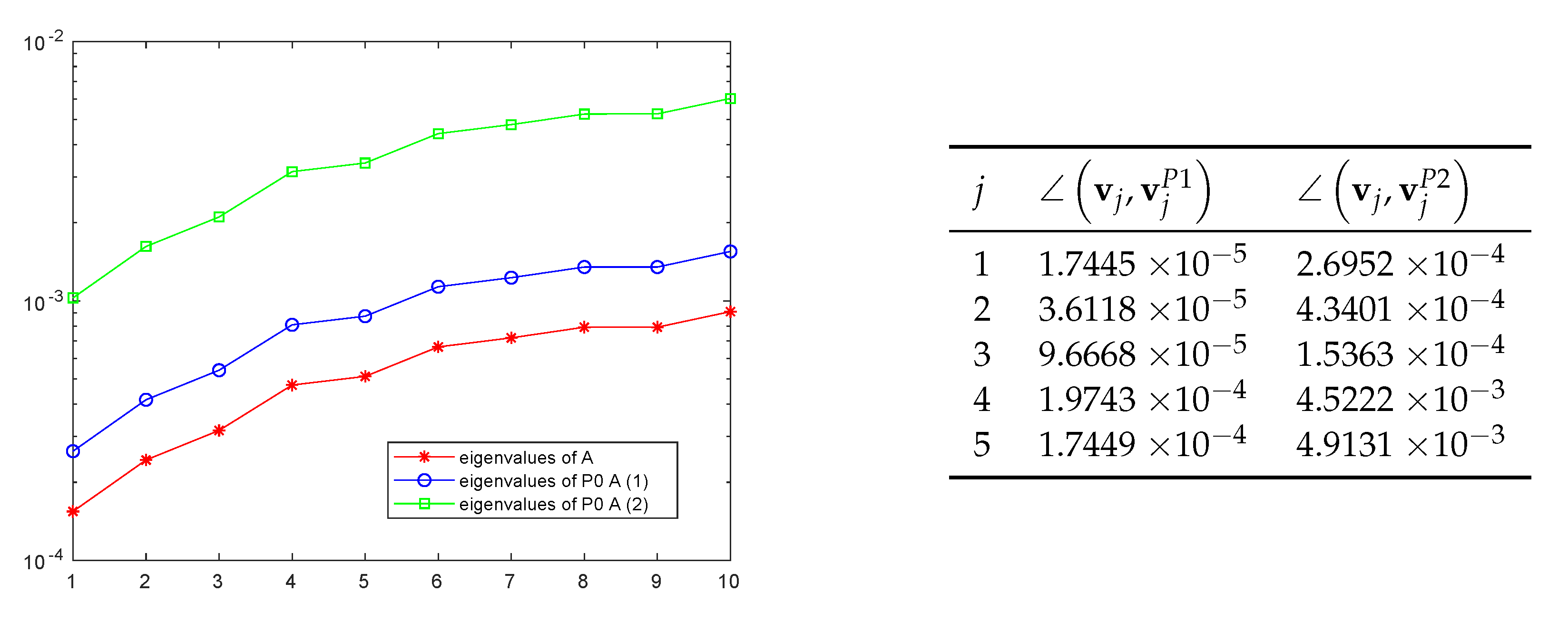
Computing a subset of the extremal eigenvectors of a given large and sparse matrix may reveal computationally costly. In the next Section we will develop some methods to save on this cost. However another possibility for the vectors w j is to use a number of the solutions to the previous linear systems in the sequence. Assume now that the matrices in the sequence are allowed to (slightly) change, that is, we want to solve
A k x k = b k , k = 1 , , N .
In this case computing the leftmost eigenvectors of A k is inefficient since this preprocessing should be done at each linear system.
We then use, for the jth linear system ( 1 < j N ), the j e f f = min { j 1 , p } solutions to the previous linear systems as columns of W W j , thus yielding:
W j = x j j e f f x j 1 .
The idea beyond this choice, which is completely cost-free, comes from the reasoning that:
  • A solution x k of the k-th linear system has with high probability non-negligible components in the directions of the leftmost eigenvectors of A k since, if b k = i = 1 n α i u i ( k ) , then x k = i = 1 n α i λ i ( k ) u i ( k ) , with the largest weights provided by the smallest eigenvalues.
  • The leftmost eigenvector of A k , k = j e f f , j 1 are good approximation of the leftmost eigenvectors of A j .
To give experimental evidence of the efficiency of this approach we report some results in solving a sequence of 30 linear systems arising from the Finite Element/Backward Euler discretization of the branched transport equation [35] which gives raise to a sequence of ( 2 × 2 ) block nonlinear systems in turn solved by the Inexact Newton method. After linearization and block Gaussian Elimination the problem reduces to the solution of a sequences of symmetric linear systems of the form
( A + B T E B ) k x = b k , k = 1 , ,
where A is SPD, B is rectangular with full row rank, E is diagonal and possibly indefinite. We take 30 consecutive linear systems from this sequence, and solve them with the minimum residual (MINRES) iterative method using as the initial preconditioner the incomplete Cholesky factorization of A with drop tolerance 10 2 and the following updates
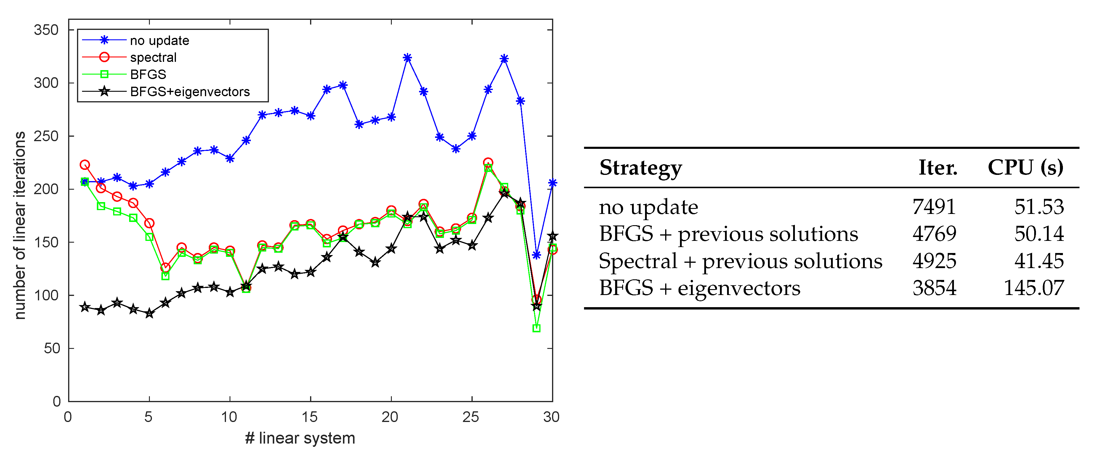
  • BFGS, with update directions as in (11).
  • Spectral preconditioner, with update directions as in (11).
  • BFGS, with the accurate leftmost eigenvectors of A k as the update directions.
The results are reported in Figure 2 where we can appreciate reduction of the number of iterations provided by the low-rank update. The (cheaper) spectral preconditioner provides as good acceleration as the BFGS approach with update directions as in (11). Moreover the number of iterations is comparable to those obtained with the “ideal” eigenvectors (which are obtained by the Matlab eigs function).

5. Cost-Free Approximation of the Leftmost Eigenpairs

The most appropriate candidate vectors for the columns of W are anyway the eigenvectors of the preconditioned matrix corresponding to the smallest eigenvalues.

The Lanczos-PCG Connection

A simple way to recover some of the extremal eigenpairs of the preconditioned matrix is to exploit the so called Lanczos connection [36,37]. During the PCG method, preconditioned with P 0 , it is possible to save the first m (scaled) preconditioned residuals as columns of a matrix V m :
V m = P 0 r 0 r 0 T P 0 r 0 , P 0 r 1 r 1 T P 0 r 1 , , P 0 r m 1 r m 1 T P 0 r m 1 .
Matrix V m is such that V m T P 0 1 V m = I m , in view of the P 0 orthogonality of the residuals generated by the PCG method. The Lanczos tridiagonal matrix can be formed using the PCG coefficients α k , β k :
T m = 1 α 0 β 1 α 0 β 1 α 0 1 α 1 + β 1 α 0 β 2 α 1 β m 1 α m 2 β m 1 α m 2 1 α m 1 + β m 1 α m 2
Matrices V m and T m obey to the classical Lanczos relation that is:
V m T A V m = T m .
The eigensolution of T m provides the eigendecomposition T m Λ m = Λ m Q m . Then, the eigenvectors corresponding to the p smallest eigenvalues are selected as p columns of matrix Q p . Finally, the columns of W p = V m Q p are expected to approximate the p leftmost eigenvectors of P 0 A .
This procedure can be implemented to a very little computational cost but it has a number of disadvantages: First, it requires the storage of m preconditioned residuals, Second, as the convergence for the Lanczos process to the smallest eigenvalues is relatively slow, it sometimes happens that PCG convergence takes place before eigenvector convergence. Third, some of the leftmost eigenpairs can be missing by the non-restarted Lanczos procedure.
To partially overcome these drawbacks in Reference [38] the authors suggest implementing a thick restart within the PCG iteration (without affecting it) and incrementally correct the eigenvector approximations during subsequent linear system solvers. The final set of directions is, in that paper, used only to deflate the initial vector and not to form a preconditioner (eigCG algorithm) in the solution of a sequence of hundreds of linear systems in lattice quantum chromodynamics.
A number of alternative ways to approximate eigenvectors during the PCG iteration can be found in the literature. In Reference [5], a technique is suggested to refine them during subsequent linear systems with the same matrix but different right-hand-sides by using the p smallest harmonic Ritz values. In this approach the vector stored within the PCG iteration are the conjugate directions p k instead of the preconditioned residuals (they actually lie in the same Krylov subspace).

6. Sequences of Nonsymmetric Linear Systems

The techniques described so far have been especially developed to accelerate the PCG method for SPD matrices. In principle they can however be extended also to nonsymmetric linear systems. Even though eigenvalues of the preconditioned matrices are not always completely informative [39,40] on the convergence of Krylov methods for such problems, in any case shifting a small number of eigenvalues towards the middle of the spectrum is usually beneficial for iterative solvers. The spectral low-rank preconditioner (SRLU) was originally presented in Reference [9] for general matrices, with no diagonalizability assumptions, to accelerate the GMRES-DR method proposed by Morgan in Reference [41]. Regarding the tuning preconditioner, the Broyden update has been successfully used, for example, in Reference [26] to accelerate the GMRES for the inner linear systems within the Arnoldi method for eigenvalue computation. For shifted linear systems, the shift invariance property of Krylov subspace is very important for building the preconditioner (see e.g., References [7,42] for details). Regarding (non necessarily low-rank) updates of a given preconditioner, we mention Reference [43] in the framework of constrained optimization, and Reference [44], which showed that (roughly) one matrix factorization and a single Krylov subspace is enough for handling the whole sequence of shifted linear systems.

7. Numerical Results

The technique previously described are very powerful when applied to sequences of linear systems where the coefficient matrix remains the same. In this case it is possible to refine the eigenvalues of the preconditioned matrix during the first linear systems solutions up to machine precision [38]. However, in most situations this high accuracy is not really needed (see the discussion in Section 4).
In this section we will consider a particular case of sequences of linear systems with (slightly) changing matrices as
A k x = b k , A k = A 0 + α k A 1 ,
which can be viewed as shifted linear systems. These sequences appear for example, in the Finite Difference or Finite Element discretization of transient PDEs or as an inner linear system within iterative eigensolvers. We will show that the low-rank techniques could be successfully employed in the acceleration of iterative methods in the solution of such linear systems.

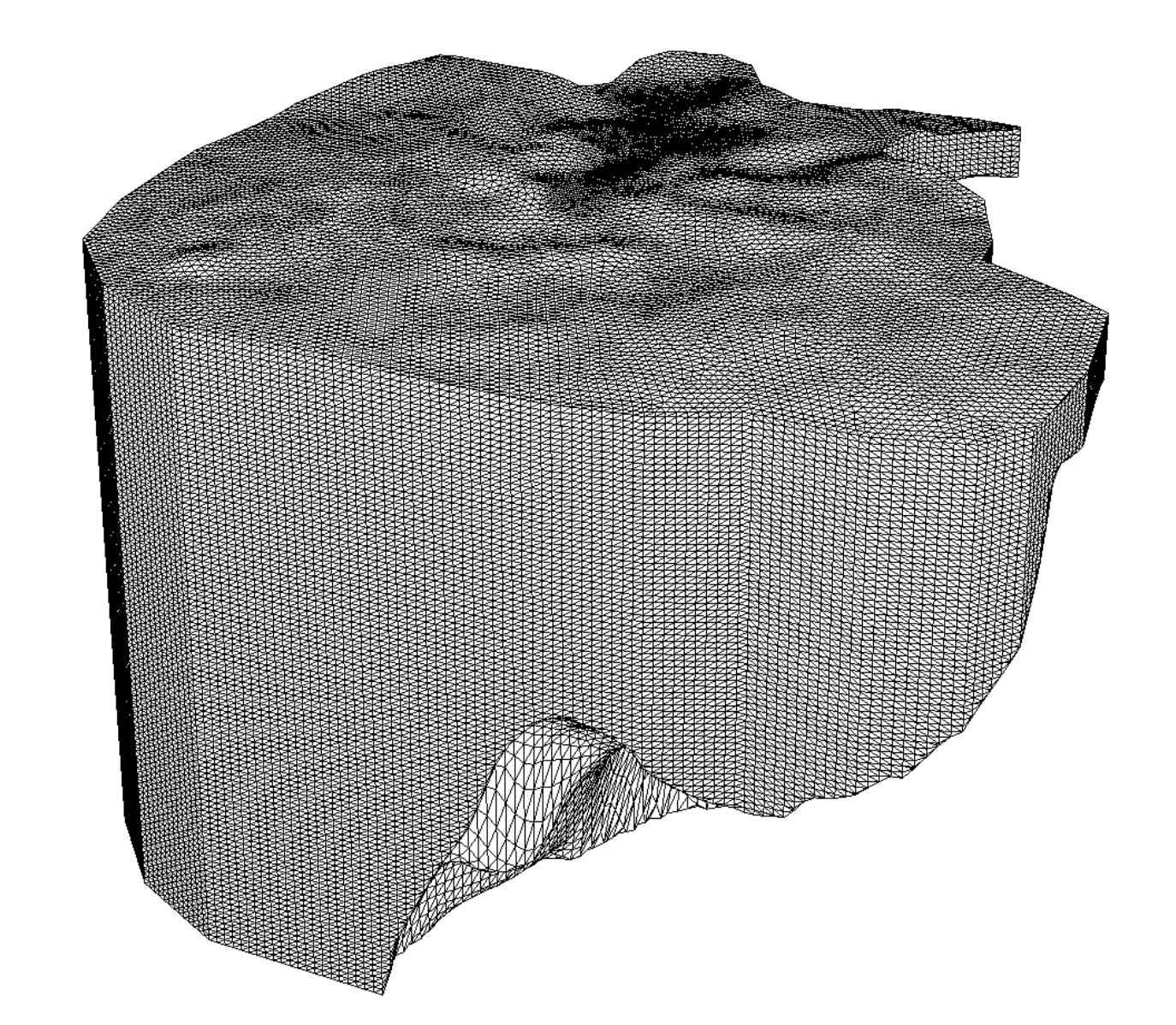
7.1. Fe Discretization of a Parabolic Equation

Consider the parabolic PDE
S h u ( x , t ) t = ( K ( x ) u ( x , t ) ) + BCs .
u is the pressure of the fluid, S h the elastic storage, K the (SPD) hydraulic conductivity tensor. This equation is used to model water pumping in the Beijing plan to predict land subsidence in that area [45]. The 3D computational domain turns out to be very heterogeneous and geometrically irregular as sketched in Figure 3:
FE discretization in space needs highly irregular tetrahedra, which, combined with the high heterogeneity of the medium, gives raise to an ill-conditioned discretized diffusion matrix. After FE discretization a system of ODEs is left:
B u ( t ) t = A u ( t ) + b ( t ) .
where A is the SPD stiffness matrix, B is the SPD mass matrix. The right-hand-side account for source terms and Neumann boundary conditions. Using a time marching scheme (e.g., Crank-Nicolson for stiff problems) yields a sequence of linear systems
( A + σ k B ) u k = b k , σ k = 2 Δ t k , k = 1 , N s t e p .
The discretized FE matrices have both n = 589,661 and a number of nonzeros n z = 8,833,795. We now report the results of a complete simulation which took N s t e p = 32 steps. The near steady state is reached after T = 36,000 days. Initially we set Δ t 1 = 60 (days). Then we incremented the timesteps as
Δ t k = min ( 1.2 Δ t k 1 , 7300 , T Δ t k 1 ) σ k = 2 Δ t k , k = 2 , , N s t e p .
This formula allows the timestep size to constantly increase and to take its largest value approaching the steady state solution. The initial preconditioner P 0 was evaluated employing the Matlab function ichol with
(1)
droptol = 10 5 applied to A 1 = A + 5 B to enhance diagonal dominance; this resulted in a triangular Cholesky factor with density 5.18 and
(2)
droptol = 10 4 applied to A 2 = A + 20 B (density 2.83 ).
We solved the first linear system to a high accuracy to assess as accurately as possible the p = 10 leftmost eigenvectors. Using the residual δ j = P 0 A w j μ j w j w j to measure the accuracy of the approximate eigenvectors we found:
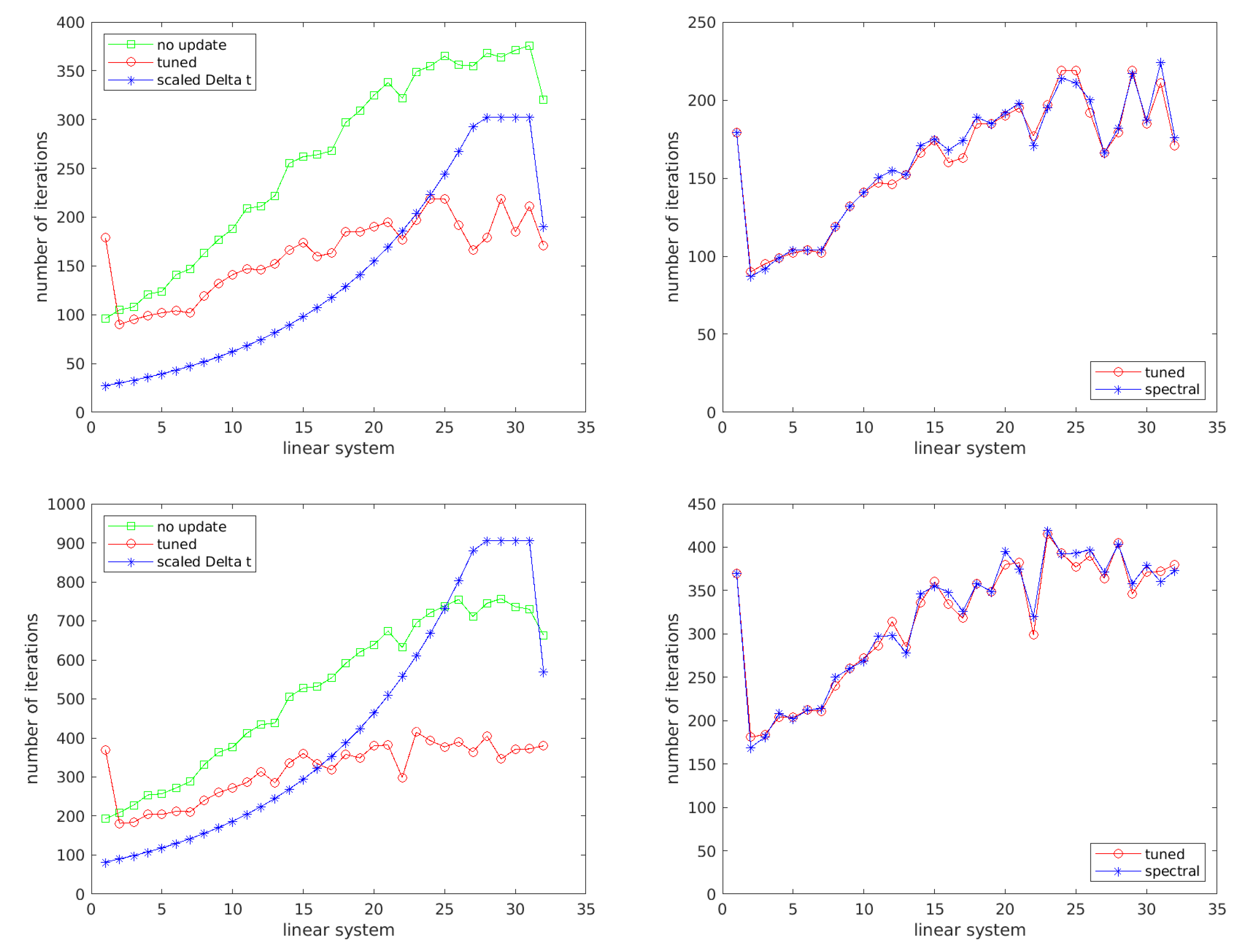
  • Case (1). 179 PCG iterations for the first linear system; δ j [ 1.1 10 3 , 5.8 10 3 ] .
  • Case (2). 370 PCG iterations for the first linear system; δ j [ 1.1 10 3 , 3.3 10 3 ] .
This set of vectors is then used to construct deflation, tuned and spectral preconditioners for all the subsequent linear systems in the sequence (with exit test on relative residual and tolerance tol = 1 e 10 ).
The results are summarized in Table 6. The eigenvectors estimated during the first linear system are adequate to accelerate the subsequent iterations for both the tuned and spectral approaches which provide an improvement in both iteration number and CPU time. Note also that the time per iteration is only slightly increased with respect to the “no update” case.
Instead, the PCG residuals obtained with the deflation preconditioner in some instances stagnate before reaching the exit test. The lack of robustness of the deflation approach is also observed in Reference [5] where the authors suggest a reorthogonalization of the residuals at the price of increasing costs per iteration and also Reference [26] in the framework of iterative eigensolvers. Regarding tuned preconditioners, SR1 is definitely superior to the BFGS approach due to its lower computational cost.
In Figure 4, left, we plot the number of iterations needed by the “no update” and tuned preconditioners for every system in the sequence compared also with the scaled Δ t k σ k 1 / 2 values (blue lines) as indicators of the increasing condition number of the coefficient matrices. On the right plot the behavior of the tuned vs spectral preconditioners is displayed, showing the substantial equivalence between the two approaches. Note finally that the PCG solver with the tuned preconditioner is almost insensitive to the increasing condition number of the matrices, displaying a number of iterations roughly constant throughout the timesteps.

7.2. Iterative Eigensolvers

When computing the smallest or a number of the interior eigenvalues of a large and sparse matrix, most iterative solvers require the solution of a shifted linear system of the type
( A σ B ) x = b .
This is true for instance in the shift-invert Arnoldi method, in the inverse power iteration, in the Rayleigh Quotient iteration. A related linear system is also to be solved within the correction equation in the Jacobi-Davidson method. Other gradient-based methods such as the Locally Optimal Block PCG method (LOBPCG) [46] or the Deflation-Accelerated Conjugate Gradient method (DACG) [47] implicitly solve a shifted linear system. The sequence of linear systems are characterized by a constant or a slowly varying parameter σ so informations on matrix A or on the pencil ( A , B ) can be profitably used for all the sequence.
We denote as 0 < λ 1 λ 2 λ m λ n its eigenvalues and v 1 , v 2 , , v m , v n the corresponding eigenvectors. Our aim is to investigate the efficiency of the SR1 tuned preconditioner in the acceleration of the so-called correction equation in the simplified Jacobi-Davidson (JD) method [48,49].
To assess eigenpair ( λ j , v j ) a number of linear systems have to be solved of the form
J k ( j ) s = ( A θ j ( k ) I ) u k ; for s u k , where
J k ( j ) = ( I QQ T ) ( A θ j ( k ) I ) ( I QQ T ) , θ j ( k ) = q ( u k ) u k T A u k u k T u k , Q = v 1 v j 1 u k .
The PCG method is proved to converge if applied to systems (13) as the Jacobian J k ( j ) is shown to be SPD in the subspace orthogonal to u k [22,49]. Following the works in [27,50], which are based on a two-stage algorithm, the columns of W are orthonormal approximate eigenvectors of A provided by a gradient method, DACG [47], satisfying
A v ˜ s = λ ˜ s v ˜ s + res s , res s τ λ s s = 1 , , m .
λ ˜ s λ s τ λ s .
These vectors are also used as initial guesses for the Newton phase. To update a given initial preconditioner for ( λ j , v j ) we use the next approximate eigenvectors v j + 1 , , v m to define an SR1 tuned preconditioner as
P j = P 0 Z Z T A W j 1 Z T , Z = P 0 A W j W j , with W j = v ˜ j + 1 v ˜ m .
We recall the following result stated in ([27], Lemma 3.1):
Lemma 1.
Let P j a block tuned preconditioner satisfying condition (17). In the hypothesis (15) each column of W j that is, v ˜ s , s = j + 1 , , m , is an approximate eigenvector of P j ( A θ j I ) satisfying
P j ( A θ j I ) v ˜ s = 1 θ j λ ˜ s v ˜ s + ε s , w i t h ε s τ λ j + 1 P j .
The effect of applying a tuned preconditioner to A θ j I is to set a number of eigenvalues of P ( A θ j I ) to a value that is close to one only under the conditions that the eigenvalues are well separated, that is, λ j λ j + 1 1 , which is not always the case in realistic problems.
In order to define a more effective preconditioner for shifted linear systems one can allow the preconditioned matrix P A to have eigenvalues different from one corresponding to the columns of matrix W. In Reference [50] a generalized block tuned (GBT) preconditioner is defined:
Definition 3.
Given a preconditioner P 0 , an n × p matrix W with full column rank, and a diagonal matrix Γ = diag ( γ 1 , , γ p ) , a generalized block tuned preconditioner for matrix A is a matrix P obtained by correcting P 0 with a low-rank matrix depending on A , W and Γ and satisfying
P A W = W Γ .
The generalized SR1 preconditioner is defined as
P = P 0 Z Π 1 Z T , where Z = P 0 A W W Γ , and Π = Z T A W .
Note that the above preconditioner is not in general symmetric as small matrix Π is not and hence its use would prevent convergence either of the DACG eigensolver or the inner PCG iteration within the Newton method. However, this drawback can be circumvented when W W j represents the matrix of the (approximate) eigenvectors corresponding to the diagonal matrix with the eigenvalues of A: Λ j = diag ( λ ˜ j + 1 , λ ˜ j + 2 , , λ ˜ m ) . In such case we can approximate Π as
Π = W j T A P A W j Γ W j T A W j W j T A P A W j Γ Λ j = Π ˜ ,
so restoring symmetry. This modified preconditioner P ˜ j = P 0 Z Π ˜ 1 Z satisfies only approximately the tuning property as
P ˜ j A v ˜ s = γ s v ˜ s + E s , E s τ λ s Z Π ˜ 1 Γ , s = j + 1 , , m .
The following theorem states that it is however possible to have p eigenvalues of the preconditioned matrix P ˜ j ( A θ j I ) very close to one depending on how the columns of matrix W approximate the eigenvectors of A. We also define the reciprocal of the relative separation between pairs of eigenvalues as
ξ j = λ j + 1 λ j + 1 λ j .
Theorem 3.
Let matrix W j be as in (17), P ˜ j an approximate GBT preconditioner satisfying condition (21), with γ s = λ ˜ s / ( λ ˜ s λ ˜ j ) , s = j + 1 , , m , then each column of W j is an approximate eigenvector of P ˜ j ( A θ j I ) corresponding to the approximate eigenvalue
μ s = λ ˜ s θ j λ ˜ s λ ˜ j .
satisfying
P ˜ j ( A θ j I ) v ˜ s = μ s v ˜ s + ε s , w i t h ε s τ λ s Z Π ˜ 1 Γ + λ j + 1 P ˜ j .
Proof. 
See Reference [50]. □
The eigenvalues μ s can be very close to one depending on the initial tolerance τ as stated in Corollary 1, under reasonable additional hypotheses
Corollary 1.
Let θ j , τ such that, for all j = 1 , , m 1 :
λ j θ j λ ˜ j ,
τ < ( 2 ξ j ) 1 ,
then
1 μ s 1 + 2 τ ( ξ j 1 ) , s = j + 1 , , m .
Proof. 
See Reference [50]. □
From Corollary 1 it is clear that μ s can be made arbitrarily close to one by appropriately reducing the tolerance τ . As an example, if ξ j = 10 2 , τ = 10 3 then all μ s are expected to be in ( 1 , 1.2 ) .
In Reference [50] (Theorem 2) is also stated that the eigenvalues of the preconditioned projected Jacobian matrix (13) are characterized in the same way as stated in Theorem 3, that is, that for a suitable function C ( τ ) , increasing in τ
P Q J k ( j ) v ˜ s = μ s v ˜ s + err , err τ C ,
where P ˜ j a generalized block tuned preconditioner, P Q = ( I QQ T ) P ˜ j ( I QQ T ) .
To limit the cost of the application of the low-rank correction it is customary to fix the maximum number of columns of matrix W j , parameter l max . Conversely, it is required to enlarge it when assessing eigenpairs with j m . The first DACG stage is hence used to compute an extra number ( win ) of approximated eigenpairs. In this way the number of columns of W j is m j = min { l max , m + win j } .
The construction (C) of P ˜ j and its application (A) as P ˜ j r are sketched below. MVP = matrix-vector products, Z j = Z 0 ( :,j+1:j+ m j ) and Π j = Π 0 ( j+1:j+ m j , j+1:j+ m j ).
PhaseWhenWhatRelevant Cost
Conce and for all
  • Z 0 = P 0 A V 0
  • Π 0 = Z 0 T A V 0
m + win MVPs and applications of P 0
( m + win ) 2 / 2 dot products.
Cfor every eigenpair
  • Z = Z j V j Γ
  • Π ˜ = Π j Γ Λ j
m j daxpys
Aat each iteration
  • h = Z T r
  • g = Π ˜ \ h
  • w = P 0 r Z g
m j dot products
1 system solve of size m j
1 application of P 0 , m j daxpys
We report from Reference [50] the results of the described preconditioner in the computation of the 20 smallest eigenpairs of matrix thermomec, which is available in the SuiteSparse Matrix Collection at https://sparse.tamu.edu/. This is a challenging test due to the high clustering of its smallest eigenvalues. The CPU times (in seconds) refer to running a Fortran 90 code on a 2 x Intel Xeon CPU E5645 at 2.40 GHz (six core) and with 4 GB RAM for each core. The exit test is on the relative eigenresidual: A u q ( u ) u q ( u ) ε = 10 8 , with q ( u ) defined in (14).
The results of the runs are displayed in Table 7 where the number of iterations (and CPU time) of the initial DACG method are reported as well as the cumulative number of iterations (and CPU time) needed for solving all the linear systems (13) within the Newton iteration for the 20 eigenpairs. Especially the second (Newton) phase takes great advantage by the GBT preconditioner as also accounted for by Figure 5 shows the number of iterations taken by the Newton phase with the fixed IC, SR1 tuned and GBT preconditioners, together the (scaled) log ξ j , which is a measure of the condition number of the inner linear systems.
The almost constant GBT curve confirms the property of this preconditioner which makes the number of iterations nearly independent on the relative separation between consecutive eigenvalues.

8. Conclusions

We have presented a general framework of updating a given preconditioner P 0 with a low-rank matrix with the aim of further clustering eigenvalues of the preconditioned matrix P 0 A . We have shown that this approach is particularly efficient when a sequence of linear systems has to be solved. In this case the cost of computation of the leftmost eigenvector of the preconditioned matrices is payed for by the number of system solutions. Alternatively, the vector forming the low-rank updates can be chosen as the previous solutions in the sequence. In summary we have reviewed three updating processes:
  • Deflation, aimed at shifting to zero a number of approximate eigenvalues of P 0 A .
  • Tuning, aimed at shifting to one a number of approximate eigenvalues of P 0 A .
  • Spectral preconditioners, aimed at adding one to a number of approximate eigenvalues of P 0 A .
The most popular choices of the vectors (such as leftmost eigenvectors of either A or P 0 A ) have been considered together with some techniques to cheaply assess them.
Finally we have considered a number of applications, such as discretization of evolutionary PDEs and solution of large eigenvalue problems. In all these applications the low-rank correction is much beneficial to reduce the number of iterations of the iterative solver of choice.
As a general recommendation we can say that accelerating a given preconditioner by a low-rank matrix can be useful when both the following situations occur:
  • A sequence of linear systems with constant or slightly varying matrices has to be solved.
  • Either the smallest or the largest eigenvalues do not form a cluster.

Funding

This research received no external funding.

Acknowledgments

The author is indebted to the reviewers whose suggestions helped improve the quality of the paper. This work was partially supported by the INdAM Research group GNCS (Year 2020 project: Optimization and Advanced Linear Algebra for Problems Governed by PDEs) and by the project funded by CARIPARO: Matrix-Free Preconditioners for Large-Scale Convex Constrained Optimization Problems (PRECOOP).

Conflicts of Interest

The author declares no conflict of interest.

References

  1. Kolotilina, L.Y.; Yeremin, A.Y. Factorized Sparse Approximate Inverse Preconditionings I. Theory. SIAM J. Matrix Anal. Appl. 1993, 14, 45–58. [Google Scholar] [CrossRef]
  2. Benzi, M.; Meyer, C.D.; Tůma, M. A Sparse Approximate Inverse Preconditioner for the Conjugate Gradient Method. SIAM J. Sci. Comput. 1996, 17, 1135–1149. [Google Scholar] [CrossRef] [Green Version]
  3. Elman, H.C.; Silvester, D.J.; Wathen, A.J. Finite Elements and Fast Iterative Solvers: With Applications in Incompressible Fluid Dynamics, 2nd ed.; Numerical Mathematics and Scientific Computation; Oxford University Press: New York, NY, USA, 2014; p. xiv+400. [Google Scholar]
  4. Nicolaides, R.A. Deflation of Conjugate Gradients with Applications to Boundary Value Problems. SIAM J. Numer. Anal. 1987, 24, 355–365. [Google Scholar] [CrossRef]
  5. Saad, Y.; Yeung, M.; Erhel, J.; Guyomarc’h, F. A deflated version of the conjugate gradient algorithm. SIAM J. Sci. Comput. 2000, 21, 1909–1926. [Google Scholar] [CrossRef] [Green Version]
  6. Morgan, R.B. A Restarted GMRES method augmented with eigenvectors. SIAM J. Matrix Anal. Appl. 1995, 16, 1154–1171. [Google Scholar] [CrossRef] [Green Version]
  7. Gu, X.M.; Huang, T.Z.; Yin, G.; Carpentieri, B.; Wen, C.; Du, L. Restarted Hessenberg method for solving shifted nonsymmetric linear systems. J. Comput. Appl. Math. 2018, 331, 166–177. [Google Scholar] [CrossRef] [Green Version]
  8. Carpentieri, B.; Duff, I.S.; Giraud, L. A class of spectral two-level preconditioners. SIAM J. Sci. Comput. 2003, 25, 749–765. [Google Scholar] [CrossRef] [Green Version]
  9. Giraud, L.; Gratton, S.; Martin, E. Incremental spectral preconditioners for sequences of linear systems. Appl. Numer. Math. 2007, 57, 1164–1180. [Google Scholar] [CrossRef]
  10. Tebbens, J.D.; Tůma, M. Efficient Preconditioning of Sequences of Nonsymmetric Linear Systems. SIAM J. Sci. Comput. 2007, 29, 1918–1941. [Google Scholar] [CrossRef] [Green Version]
  11. Duintjer Tebbens, J.; Tůma, M. Preconditioner updates for solving sequences of linear systems in matrix-free environment. Numer. Linear Algebra Appl. 2010, 17, 997–1019. [Google Scholar] [CrossRef] [Green Version]
  12. Benzi, M.; Bertaccini, D. Approximate inverse preconditioning for shifted linear systems. BIT 2003, 43, 231–244. [Google Scholar] [CrossRef]
  13. Bertaccini, D. Efficient preconditioning for sequences of parametric complex symmetric linear systems. Electron. Trans. Numer. Anal. 2004, 18, 49–64. [Google Scholar]
  14. Dostál, Z. Conjugate gradient method with preconditioning by projector. Int. J. Comput. Math. 1988, 23, 315–323. [Google Scholar] [CrossRef]
  15. Mansfield, L. On the use of deflation to improve the convergence of conjugate gradient iteration. Commun. Appl. Numer. Methods 1988, 4, 151–156. [Google Scholar] [CrossRef]
  16. Frank, J.; Vuik, C. On the Construction of Deflation-Based Preconditioners. SIAM J. Sci. Comput. 2001, 23, 442–462. [Google Scholar] [CrossRef] [Green Version]
  17. Gutknecht, M.H. Spectral deflation in Krylov solvers: A theory of coordinate space based methods. Electron. Trans. Numer. Anal. 2012, 39, 156–185. [Google Scholar]
  18. Freitag, M.A.; Spence, A. Convergence of inexact inverse iteration with application to preconditioned iterative solves. BIT Numer. Math. 2007, 47, 27–44. [Google Scholar] [CrossRef] [Green Version]
  19. Freitag, M.A.; Spence, A. A tuned preconditioner for inexact inverse iteration applied to Hermitian eigenvalue problems. IMA J. Numer. Anal. 2008, 28, 522–551. [Google Scholar] [CrossRef]
  20. Bergamaschi, L.; Bru, R.; Martínez, A.; Putti, M. Quasi-Newton preconditioners for the inexact Newton method. Electron. Trans. Numer. Anal. 2006, 23, 76–87. [Google Scholar]
  21. Bergamaschi, L.; Bru, R.; Martínez, A. Low-Rank Update of Preconditioners for the Inexact Newton Method with SPD Jacobian. Math. Comput. Model. 2011, 54, 1863–1873. [Google Scholar] [CrossRef]
  22. Bergamaschi, L.; Martínez, A. Efficiently preconditioned Inexact Newton methods for large symmetric eigenvalue problems. Optim. Methods Softw. 2015, 30, 301–322. [Google Scholar] [CrossRef] [Green Version]
  23. Bergamaschi, L.; Bru, R.; Martínez, A.; Mas, J.; Putti, M. Low-rank Update of Preconditioners for the nonlinear Richard’s Equation. Math. Comput. Model. 2013, 57, 1933–1941. [Google Scholar] [CrossRef]
  24. Bergamaschi, L.; Bru, R.; Martínez, A.; Putti, M. Quasi-Newton Acceleration of ILU Preconditioners for Nonlinear Two-Phase Flow Equations in Porous Media. Adv. Eng. Softw. 2012, 46, 63–68. [Google Scholar] [CrossRef]
  25. Martínez, A. Tuned preconditioners for the eigensolution of large SPD matrices arising in engineering problems. Numer. Linear Algebra Appl. 2016, 23, 427–443. [Google Scholar] [CrossRef]
  26. Freitag, M.A.; Spence, A. Shift-invert Arnoldi’s method with preconditioned iterative solves. SIAM J. Matrix Anal. Appl. 2009, 31, 942–969. [Google Scholar] [CrossRef]
  27. Bergamaschi, L.; Martínez, A. Two-stage spectral preconditioners for iterative eigensolvers. Numer. Linear Algebra Appl. 2017, 24, e2084. [Google Scholar] [CrossRef]
  28. Bergamaschi, L.; Marín, J.; Martínez, A. Compact Quasi-Newton preconditioners for SPD linear systems. arXiv 2020, arXiv:2001.01062. [Google Scholar]
  29. Nabben, R.; Vuik, C. A comparison of deflation and the balancing preconditioner. SIAM J. Sci. Comput. 2006, 27, 1742–1759. [Google Scholar] [CrossRef]
  30. Xue, F.; Elman, H.C. Convergence analysis of iterative solvers in inexact Rayleigh quotient iteration. SIAM J. Matrix Anal. Appl. 2009, 31, 877–899. [Google Scholar] [CrossRef] [Green Version]
  31. Bergamaschi, L.; De Simone, V.; di Serafino, D.; Martínez, A. BFGS-like updates of constraint preconditioners for sequences of KKT linear systems. Numer. Linear Algebra Appl. 2018, 25, 1–19. [Google Scholar] [CrossRef]
  32. Gratton, S.; Mercier, S.; Tardieu, N.; Vasseur, X. Limited memory preconditioners for symmetric indefinite problems with application to structural mechanics. Numer. Linear Algebra Appl. 2016, 23, 865–887. [Google Scholar] [CrossRef] [Green Version]
  33. Bergamaschi, L.; Gondzio, J.; Martínez, A.; Pearson, J.; Pougkakiotis, S. A New Preconditioning Approach for an Interior Point-Proximal Method of Multipliers for Linear and Convex Quadratic Programming. arXiv 2019, arXiv:1912.10064. [Google Scholar]
  34. Duff, I.S.; Giraud, L.; Langou, J.; Martin, E. Using spectral low rank preconditioners for large electromagnetic calculations. Int. J. Numer. Methods Eng. 2005, 62, 416–434. [Google Scholar] [CrossRef] [Green Version]
  35. Bergamaschi, L.; Facca, E.; Martínez, A.; Putti, M. Spectral preconditioners for the efficient numerical solution of a continuous branched transport model. J. Comput. Appl. Math. 2019, 254, 259–270. [Google Scholar] [CrossRef]
  36. Golub, G.H.; van Loan, C.F. Matrix Computation; Johns Hopkins University Press: Baltimore, MD, USA, 1991. [Google Scholar]
  37. Saad, Y. Iterative Methods for Sparse Linear Systems, 2nd ed.; SIAM: Philadelphia, PA, USA, 2003. [Google Scholar]
  38. Stathopoulos, A.; Orginos, K. Computing and deflating eigenvalues while solving multiple right-hand side linear systems with an application to quantum chromodynamics. SIAM J. Sci. Comput. 2010, 32, 439–462. [Google Scholar] [CrossRef]
  39. Greenbaum, A. Iterative Methods for Solving Linear Systems; SIAM: Philadelphia, PA, USA, 1997. [Google Scholar]
  40. Embree, M. How Descriptive Are GMRES Convergence Bounds? Technical Report; Technical Report; Oxford University Computing Laboratory: Oxford, UK, 1999. [Google Scholar]
  41. Morgan, R.B. GMRES with Deflated Restarting. SIAM J. Sci. Comput. 2002, 24, 20–37. [Google Scholar] [CrossRef] [Green Version]
  42. Simoncini, V. Restarted Full Orthogonalization Method for Shifted Linear Systems. BIT Numer. Math. 2003, 43, 459–466. [Google Scholar] [CrossRef]
  43. Bellavia, S.; De Simone, V.; Di Serafino, D.; Morini, B. Efficient preconditioner updates for shifted linear systems. SIAM J. Sci. Comput. 2011, 33, 1785–1809. [Google Scholar] [CrossRef]
  44. Luo, W.H.; Huang, T.Z.; Li, L.; Zhang, Y.; Gu, X.M. Efficient preconditioner updates for unsymmetric shifted linear systems. Comput. Math. Appl. 2014, 67, 1643–1655. [Google Scholar] [CrossRef]
  45. Zhu, L.; Gong, H.; Li, X.; Wang, R.; Chen, B.; Dai, Z.; Teatini, P. Land subsidence due to groundwater withdrawal in the northern Beijing plain, China. Eng. Geol. 2015, 193, 243–255. [Google Scholar] [CrossRef]
  46. Knyazev, A. Toward the optimal preconditioned eigensolver: Locally optimal block preconditioned conjugate gradient method. SIAM J. Sci. Comput. 2001, 23, 517–541. [Google Scholar] [CrossRef]
  47. Bergamaschi, L.; Gambolati, G.; Pini, G. Asymptotic Convergence of Conjugate Gradient Methods for the Partial Symmetric Eigenproblem. Numer. Linear Algebra Appl. 1997, 4, 69–84. [Google Scholar] [CrossRef]
  48. Sleijpen, G.L.G.; van der Vorst, H.A. A Jacobi-Davidson method for Linear Eigenvalue Problems. SIAM J. Matrix Anal. Appl. 1996, 17, 401–425. [Google Scholar] [CrossRef]
  49. Notay, Y. Combination of Jacobi-Davidson and conjugate gradients for the partial symmetric eigenproblem. Numer. Linear Algebra Appl. 2002, 9, 21–44. [Google Scholar] [CrossRef]
  50. Bergamaschi, L.; Martínez, A. Generalized Block Tuned preconditioners for SPD eigensolvers. Springer INdAM Ser. 2019, 30, 237–252. [Google Scholar]
Figure 1. Eigenvalues and angle between eigenvectors of A and IC-preconditioned A.
Algorithms 13 00100 g001
Figure 2. Number of iterations to solve each linear system in the sequence by MINRES with: no update, BFGS update with previous solutions, spectral update with previous solutions, BFGS update with leftmost eigenvectors. On the right also the CPU time is reported.
Algorithms 13 00100 g002
Figure 3. 3D domain and triangulation.
Algorithms 13 00100 g003
Figure 4. Number of iterations for each linear system in the sequence and various preconditioning strategies. Initial preconditioner: IC ( A 1 , 1 e 5 ) (upper plots) and IC ( A 2 , 1 e 4 ) lower plots.
Algorithms 13 00100 g004
Figure 5. Number of iterations for the Newton phase with fixed, SR1 tuned and generalized block tuned (GBT) preconditioners. In red the (scaled) logarithm of the indicator ξ j .
Algorithms 13 00100 g005
Table 1. Direct, inverse and block versions of the Broyden (nonsymmetric) update.
direct M = M 0 + ( A M 0 ) w w T w T w M w = A w
inverse P = P 0 ( P 0 A w w ) w T P 0 w T P 0 A w P A w = w
block P = P 0 ( P 0 A W W ) W T P 0 A W 1 W T P 0 P A W = W
Table 2. Direct, inverse and block versions of the SR1 update.
direct M = M 0 + u u T w T u , u = ( A M 0 ) w
inverse P = P 0 z z T z T A w , z = P 0 A w w
block P = P 0 Z Z T A W 1 Z T , Z = P 0 A W W
Table 3. Direct, inverse and block versions of the BFGS update.
direct M = M 0 + ( A w ) T A w w T A w M 0 w w T M 0 w T M 0 w
inverse P = w w T w T A w + I w w T A w T A w P 0 I A w w T w T A w
block P = W Π 1 W T + H P 0 H T    Π = W T A W   (1) H = I W Π 1 W T A
Table 4. Influence of accuracy of the eigenvectors of P 0 A on the efficiency of the low-rank preconditioners. PCG iterations with various updating strategies are reported.
No UpdateTunedDeflatedSpectral
exact466254254254
δ = 0.01 466261259290
δ = 0.05 466378260286
Table 5. Influence of accuracy of the eigenvectors of A on the efficiency of the low-rank preconditioners. PCG iterations with various updating strategies are reported.
No UpdateTunedDeflatedSpectral
exact466254254254
δ = 10 3 466296296297
δ = 0.01 466362361369
Table 6. Number of iterations and total CPU time for solving the sequence (12) of shifted linear system. = for some of the system in the sequence convergence not achieved.
IC ( A 1 , 1 e 5 )IC ( A 2 , 1 e 4 )
update# itsCPUCPU per it.# itsCPUCPU per it.
no update8231805.80.098165821177.20.071
spectral5213557.30.10710225817.50.080
SR1 tuned5161551.70.10710152811.40.080
BFGS tuned5178612.30.11810198924.60.091
deflated
Table 7. Timings and iterations for the DACG -Newton method for the computation of m = 20 eigenpairs of matrix thermomec. In boldface the smallest overall number of iterations and CPU time.
DACGNewtonTotal
IterationsCPU
Prec.win l max τ Its.CPUOUTInner MVPCPU
Fixed00 10 4 151015.86153262834.12429152.97
SR1 Tuned1010 10 3 133514.89137218732.19365951.48
GBT510 10 3 77711.16446079.42142820.74

