Development of a Family of Jarratt-Like Sixth-Order Iterative Methods for Solving Nonlinear Systems with Their Basins of Attraction

Abstract

We develop a family of three-step sixth order methods with generic weight functions employed in the second and third sub-steps for solving nonlinear systems. Theoretical and computational studies are of major concern for the convergence behavior with applications to special cases of rational weight functions. A number of numerical examples are illustrated to confirm the convergence behavior of local as well as global character of the proposed and existing methods viewed through the basins of attraction.

1. Introduction

Since exact solutions for nonlinear equations are rarely available, we usually resort to their numerical solutions. To locate the desired numerical roots, many authors [1,2,3,4,5,6,7,8,9] have developed high-order iterative methods including optimal eighth-order ones [10,11,12,13,14,15].

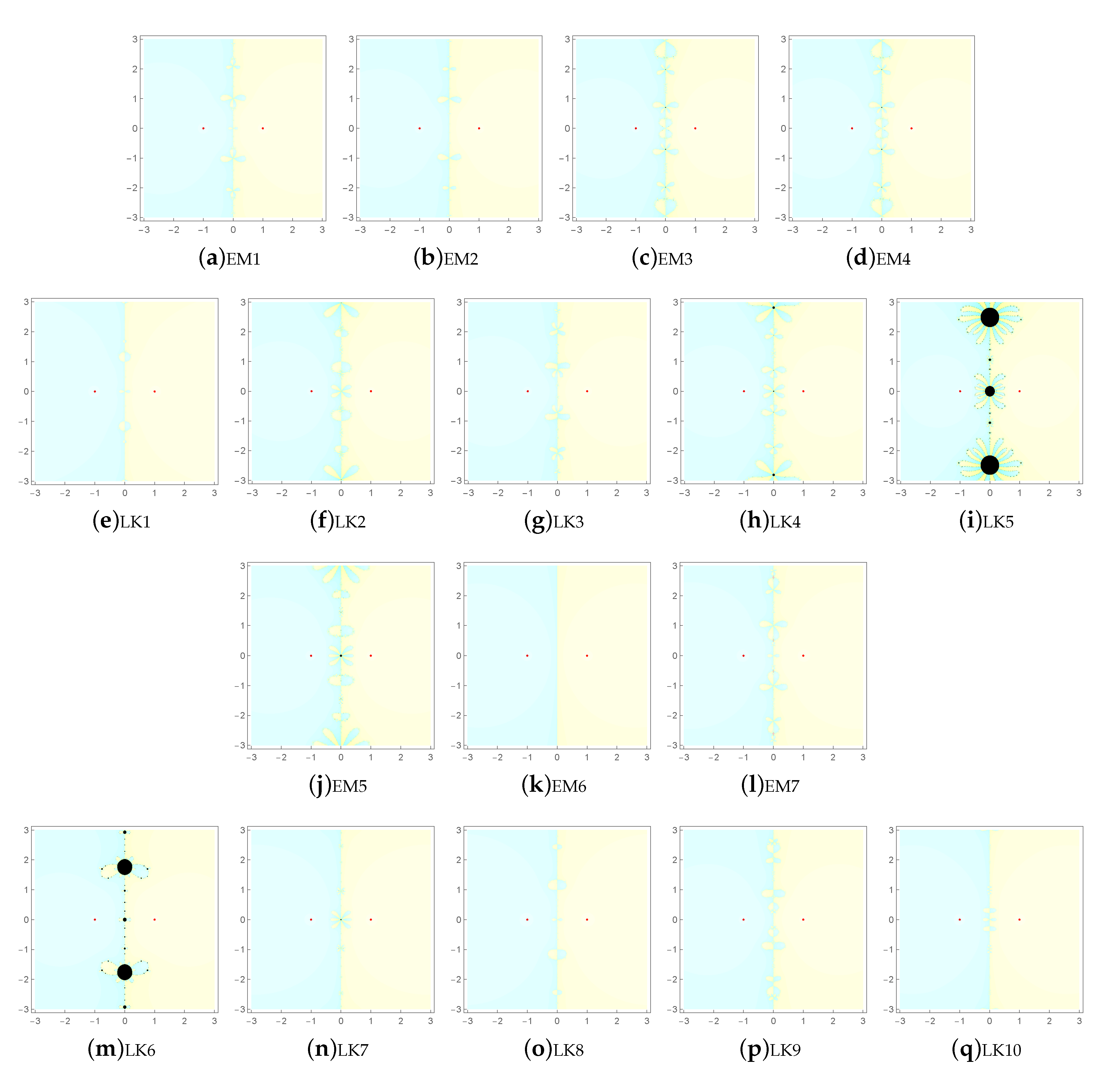
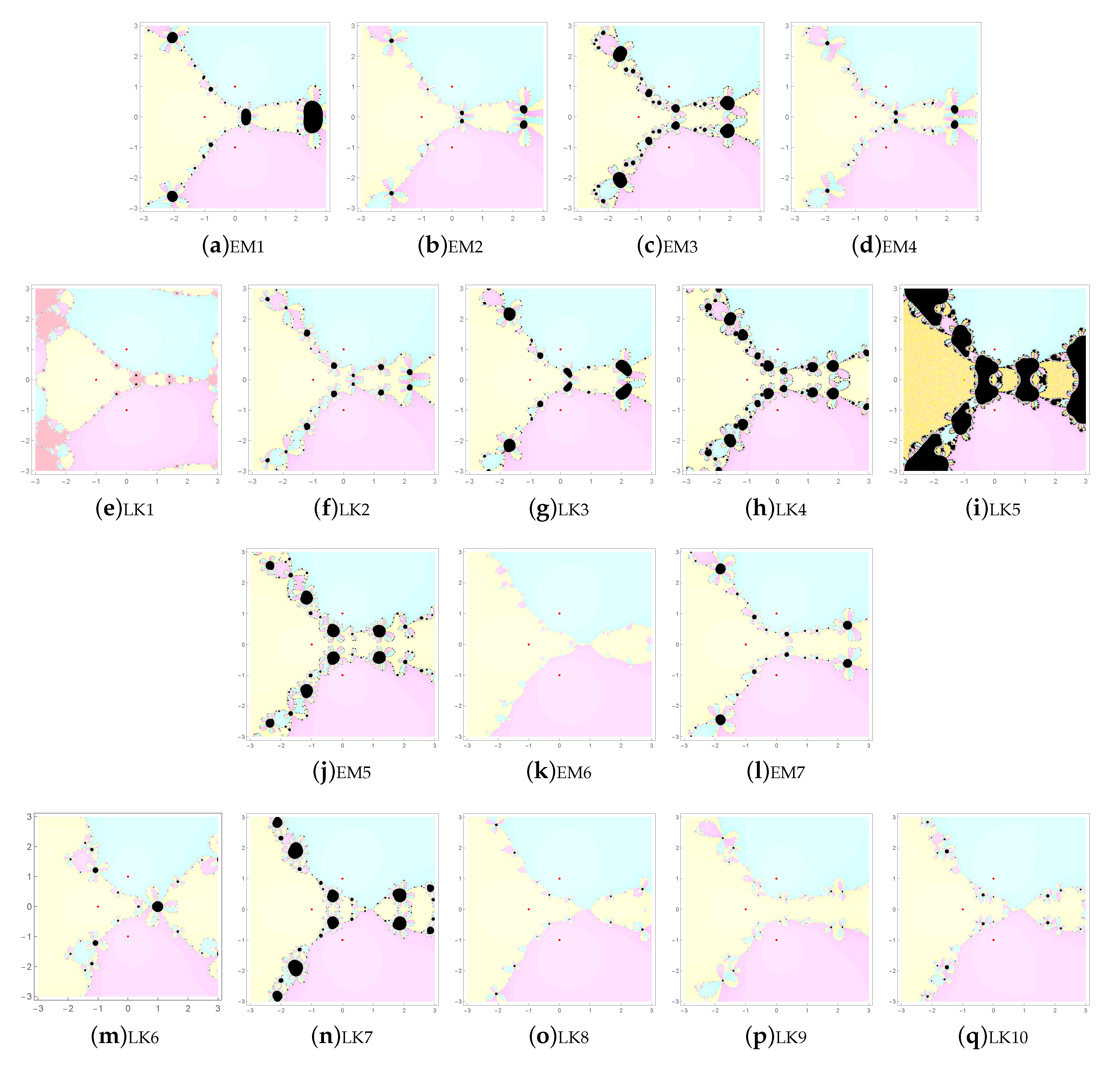
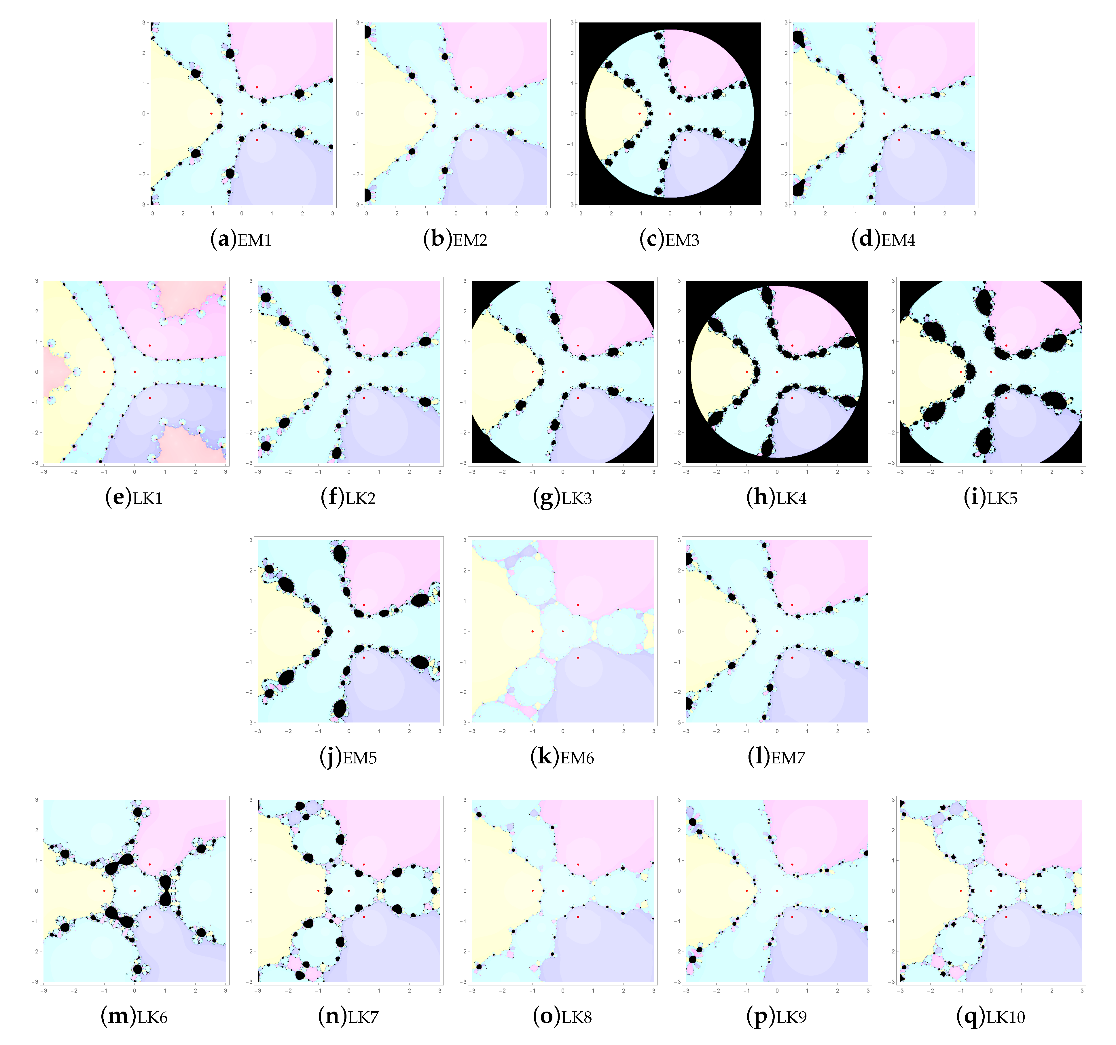
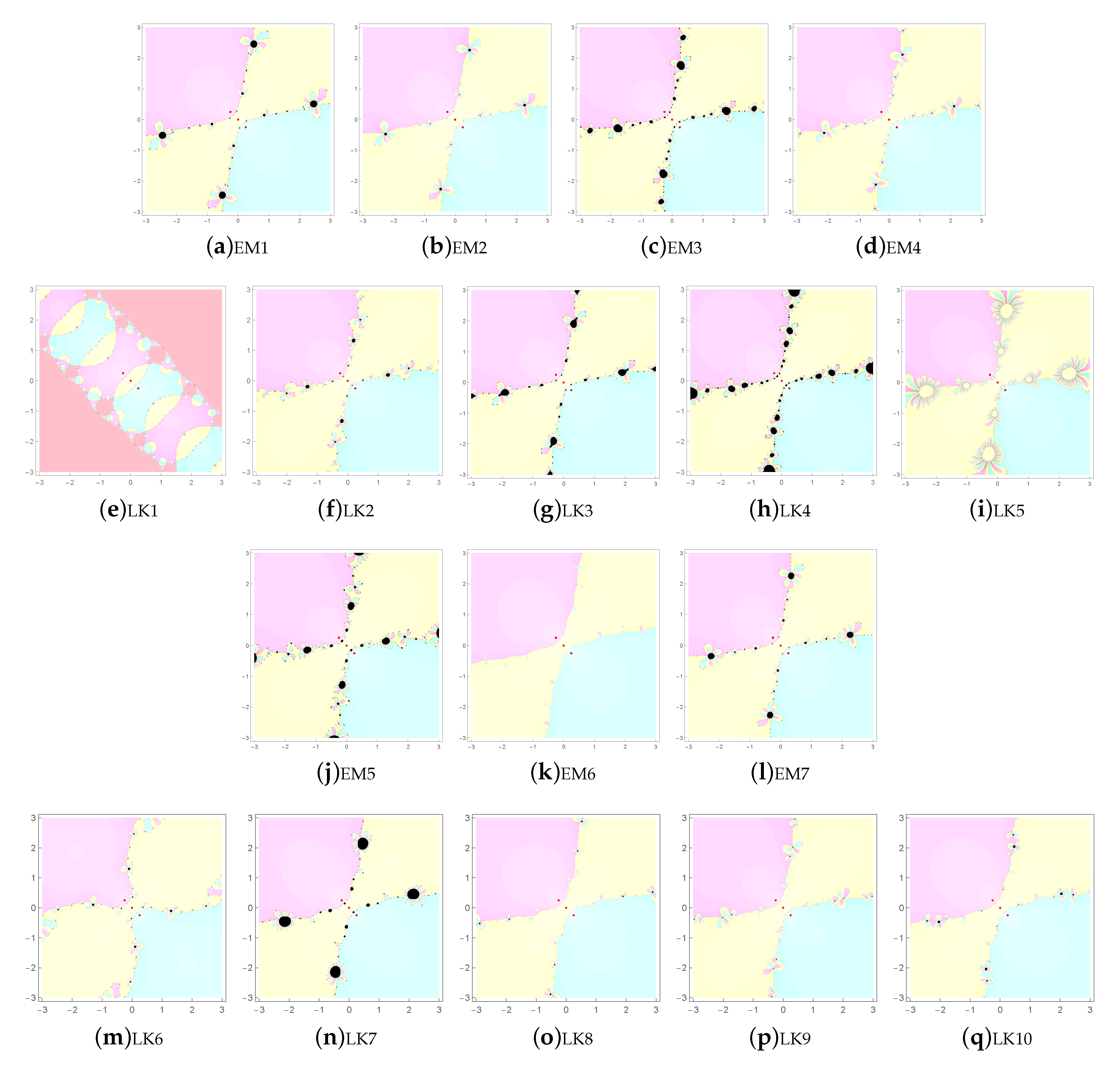
This paper is devoted to devise a class of sixth-order iterative root-finders for nonlinear systems by employing a three-step weighted Jarratt-like method below:

$$\left\{\begin{array}{c}{y}_n=x_n-\gamma ·{f^{\prime }(x_n)}^{-1}f(x_n),\gamma \in \mathbb{R},\hfill \\ z_n=x_n-T_f(s)·{f^{\prime }(x_n)}^{-1}f(x_n),\hfill \\ x_{n+1}=z_n-L_f(s)·{f^{\prime }(x_n)}^{-1}f(z_n),\hfill \end{array}\right.$$

(1)

where $s={f^{\prime }(x_n)}^{-1}{f}^{\prime }(y_n)$, $\gamma$ is a parameter to be determined later and $T_f,L_f:\mathbb{C}\to \mathbb{C}$ are weight functions being analytic [16,17,18] in a neighborhood of 1. Note that Scheme (1) uses two functional values as well as two derivatives. We are certainly able to introduce generic weight functions using one derivative and three functional values to develop general optimal eighth-order methods that covers the existing ones for the zero of a given scalar function. However, expanding such approach to a nonlinear system requires different weight functions. For unified analysis to be performed in both scalar and vector functions, we aim to develop a family of Jarratt-like sixth-order iterative methods by maintaining the same form of weight functions with two derivatives as well as two functional values. This extension to nonlinear systems is the main strength of this paper.

The robustness of the current analysis presented here covers most existing studies on higher-order root-finders using two derivatives and two function values for both scalar and vector equations. The results of Theorem 1 give us not only fairly generic scalar function solvers, but also some advantage of extending to a nonlinear system with any finite dimension. Such an extension is evidently characterized by Theorem 2 to be studied in this analysis.

Our major aim is not only to design a class of sixth-order methods by fully specifying the algebraic structure of generic weight functions $T_f(s)$ and $L_f(s)$, but also to investigate their basins of attraction behind the extraneous fixed points [19] when applied to polynomials. The last sub-step of (1) in the form of weighted Newton’s method is clearly more convenient in dealing with extraneous fixed points which are the roots of the weight function $T_f(s)+L_f(s)·\frac{f(z)}{f(x)}$.

The extraneous fixed points may lead us to attractive, indifferent, repulsive and chaotic orbits via the related basins of attraction.

Section 2 investigates the main theorem regarding the convergence behavior with the desired forms of weight functions, while Section 3 deals with special cases of weight functions that can cover many of the existing studies using two derivatives and two functional evaluations. Section 4 discusses the computational and long-term orbit behavior of the proposed iterative methods regarding scalar functions. Section 5 presents numerical experiments in a d-dimensional Euclidean space by solving a system of nonlinear vector equations $f:{\mathbb{R}}^d\to {\mathbb{R}}^d$ encountered in a real life with $d\in \{3,4,9,10\}$. In addition, computational efficiency is addressed with issues related to the accuracy and applicability of the proposed methods. Concluding remarks are stated in Section 6.

2. Main Theorem

The main theorem for a nonlinear scalar equation will be pursued and extended later in Section 5 to a system of nonlinear vector equations:

Theorem 1.

Assume that $f:\mathit{D}\subset \mathbb{C}\to \mathbb{C}$ has a simple root α and is analytic in a region D containing α. Let ${\theta }_j=\frac{f^{(j)}(\alpha )}{j!f^{\prime }(\alpha )}$ for $j=2,3,\cdots$. Let $x_0$ be an initial guess chosen in a sufficiently small neighborhood of α. Let $T_f,L_f:\mathbb{C}\to \mathbb{C}$ be analytic in a neighborhood of 1. Let $T_i=\frac{1}{i!}\frac{d^i}{d{s}^i}{T}_f(s){|}_{s=1}$ and $L_i=\frac{1}{i!}\frac{d^i}{d{s}^i}{L}_f(s){|}_{s=1}$ for $0\le i\le 5$. If $T_0=1,T_1=-\frac{1}{2\gamma },L_0=1,L_1=-\frac{1}{\gamma }$, then iterative scheme (1) defines a family of fifth-order methods for $\gamma \in \mathbb{R}-\left\{0\right\}$. If we add further constraints either with $\{\gamma =\frac{2}{3},T_2=\frac{9}{8},|T_3|<\infty ,|L_2|<\infty \}$ or with $\{\gamma =1,L_2=\frac{3}{2},|L_3|<\infty ,|T_2|<\infty \}$, then iterative scheme (1) reduces to a family of sixth-order methods satisfying the error equation below. For $n=0,1,2,\cdots ,$

$$e_{n+1}=\left\{\begin{array}{c}-\frac{1}{243}\left[2(-27+8L_2){\theta }_2^2+9{\theta }_3\right]·\left[(135+64T_3){\theta }_2^3-27{\theta }_2{\theta }_3+3{\theta }_4\right]e_n^6+O(e_n^7),if\gamma =\frac{2}{3},\hfill \\ \left[4(1-2T_2)(9+4L_3+2T_2){\theta }_2^5+4(1+L_3+3T_2){\theta }_2^3{\theta }_3-\frac{5}{4}{\theta }_2{\theta }_3^2\right]e_n^6+O(e_n^7),if\gamma =1.\hfill \end{array}\right.$$

(2)

Proof. 

Taylor series expansion of $f(x_n)$ about $\alpha$ up to sixth-order terms with $f(\alpha )=0$ leads us to the following:

$$f(x_n)=f^{\prime }(\alpha )[e_n+{\theta }_2{e}_n^2+{\theta }_3{e}_n^3+{\theta }_4{e}_n^4+{\theta }_5{e}_n^5+{\theta }_6{e}_n^6+O(e_n^7)].$$

(3)

It follows that

$$f^{\prime }(x_n)=f^{\prime }(\alpha )[1+2{\theta }_2{e}_n+3{\theta }_3{e}_n^2+4{\theta }_4{e}_n^3+5{\theta }_5{e}_n^4+6{\theta }_6{e}_n^5+O(e_n^6)].$$

(4)

For brevity of notation, we denote $e_n$ by e, unless otherwise specified from now on. Symbolic computation of Mathematica [20] yields:

$$y_n=x_n-\gamma \frac{f(x_n)}{f^{\prime }(x_n)}=\alpha +(1-\gamma )e+\gamma {\theta }_2{e}^2-2\gamma ({\theta }_2^2-{\theta }_3)e^3+Y_4{e}^4+Y_5{e}^5+Y_6{e}^6+O(e^7),$$

(5)

where $Y_4=\gamma (4{\theta }_2^3-7{\theta }_2{\theta }_3+3{\theta }_4),Y_5=-2\gamma (4{\theta }_2^4-10{\theta }_2^2{\theta }_3+3{\theta }_3^2+5{\theta }_2{\theta }_4-2{\theta }_5)$, $Y_6=\gamma (16{\theta }_2^5-52{\theta }_2^3{\theta }_3+33{\theta }_2{\theta }_3^2+28{\theta }_2^2{\theta }_4-17{\theta }_3{\theta }_4-13{\theta }_2{\theta }_5+5{\theta }_6)$.

In view of the fact that $f^{\prime }(y_n)=f^{\prime }(x_n){|}_{e_n\to (y_n-\alpha )}$, we get:

$$f^{\prime }(y_n)=f^{\prime }(\alpha )[1-2(\gamma -1){\theta }_{2}e+[2\gamma {\theta }_2^2+3{(\gamma -1)}^2{\theta }_3]e^2+{\mathsf{\Sigma }}_{i=3}^5{D}_i{e}^i+O(e^6)],$$

(6)

where $D_i=D_i(\gamma ,{\theta }_2,{\theta }_3,\cdots ,{\theta }_6)$ for $3\le i\le 5$. Hence, we have:

$$s=\frac{f^{\prime }(y_n)}{f^{\prime }(x_n)}=1-2\gamma {\theta }_{2}e+3\gamma [2{\theta }_2^2+(-2+\gamma ){\theta }_3])e^2+{\mathsf{\Sigma }}_{i=3}^5{E}_i{e}^i+O(e^6),$$

(7)

where $E_i=E_i(\gamma ,{\theta }_2,{\theta }_3,\cdots ,{\theta }_6)$ for $3\le i\le 5$.

Noting that $s=1+O(e)$ and $\frac{f(x_n)}{f^{\prime }(x_n)}=O(e)$, we need a Taylor expansion of $T_f(s)$ about $s=1$ up to fifth-order terms:

$$T_f(s)=T_0+T_1(s-1)+T_2{(s-1)}^2+T_3{(s-1)}^3+T_4{(s-1)}^4+T_5{(s-1)}^5+O(e^6).$$

(8)

Thus, we find

$$z_n=x_n-T_f(s)·\frac{f(x_n)}{f^{\prime }(x_n)}=\alpha +(1-T_0)e+(T_0+2T_1\gamma ){\theta }_2{e}^2+$$

$$[-2T_0({\theta }_2^2-{\theta }_3)-\gamma (8T_1{\theta }_2^2+4T_2\gamma {\theta }_2^2+3T_1(-2+\gamma ){\theta }_3)]e^3+{\mathsf{\Sigma }}_{i=4}^6{W}_i{e}^i+O(e^7),$$

(9)

where $W_i=W_i(\gamma ,{\theta }_2,{\theta }_3,\cdots ,{\theta }_6,T_0,\cdots ,T_5)$ for $4\le i\le 6$.

In view of the fact that $f(z_n)=f(x_n){|}_{e_n\to (z_n-\alpha )}$, we get:

$$f(z_n)=f^{\prime }(\alpha )[(1-T_0)e+[{(1-T_0)}^2{\theta }_2+(T_0+2T_1\gamma ){\theta }_2]e^2+{\mathsf{\Sigma }}_{i=3}^6{F}_i{e}^i+O(e^7)],$$

(10)

where $F_i=F_i(\gamma ,{\theta }_2,{\theta }_3,\cdots ,{\theta }_6,T_0,\cdots ,T_5)$ for $3\le i\le 6$. Noting that $s=O(1)$ and $\frac{f(z_n)}{f^{\prime }(x_n)}=O(e)$, we need a Taylor expansion of $L_f(s)$ about $s=1$ up to fifth-order terms:

$$L_f(s)=L_0+L_1(s-1)+L_2{(s-1)}^2+L_3{(s-1)}^3+L_4{(s-1)}^4+L_5{(s-1)}^5+O(e^6).$$

(11)

Hence, we have:

$$x_{n+1}=z_n-L_f(s)·\frac{f(z_n)}{f^{\prime }(x_n)}=\alpha +(L_0-1)(T_0-1)e$$

$$+[(T_0-2L_1{T}_0\gamma +2(L_1+T_1)\gamma -L_0(-1+T_0+T_0^2+2T_1\gamma )]{\theta }_2{e}^2+{\mathsf{\Sigma }}_{i=3}^6{G}_i{e}^i+O(e^7),$$

(12)

where $G_i=G_i(\gamma ,{\theta }_2,{\theta }_3,\cdots ,{\theta }_6,T_0,\cdots ,T_5,L_0,\cdots ,L_5)$ for $3\le i\le 6$.

By taking

$$T_0=1,T_1=-\frac{1}{2\gamma },L_0=1,L_1=-\frac{1}{\gamma },$$

(13)

we further obtain

$$x_{n+1}=\alpha +[4(-3+2L_2{\gamma }^2)(-1+2T_2{\gamma }^2){\theta }_2^4+(-12+15\gamma +4(L_2+3T_2){\gamma }^2-6(L_2+2T_2){\gamma }^3){\theta }_2^2{\theta }_3$$

$$+\frac{3}{2}(\gamma -1)(3\gamma -2){\theta }_3^2]e^5+G_6{e}^6+O(e^7).$$

(14)

From $(\gamma -1)(3\gamma -2)=0$, we find two sets of relations:

$$\{\gamma =\frac{2}{3},T_2=\frac{9}{8}\},\{\gamma =1,L_2=\frac{3}{2}\}$$

for vanishing the fifth-order term in (14). Hence, we eventually have two sets of relations:

$$\{\gamma =\frac{2}{3},T_0=1,T_1=-\frac{3}{4},T_2=\frac{9}{8},L_0=1,L_1=-\frac{3}{2}\},$$

$$\{\gamma =1,T_0=1,T_1=-\frac{1}{2},L_0=1,L_1=-1,L_2=\frac{3}{2}\},$$

which are substituted into $G_6$ in (14) and lead us to the desired relation (2) with $\left\{\right|T_3|<\infty ,|L_2|<\infty \}$ when $\gamma =\frac{2}{3}$, or with $\left\{\right|L_3|<\infty ,|T_2|<\infty \}$ when $\gamma =1$. □

Remark 1.

The fifth-order expansion of the weight functions is considered due to the fact that $s=1+O(e)$ and $\frac{f(z_n)}{f^{\prime }(x_n)}=O(e)$ or $\frac{f(x_n)}{f^{\prime }(x_n)}=O(e)$. However, the result of Theorem 1 shows that $z=O(e^k),\frac{f(z_n)}{f^{\prime }(x_n)}=O(e^k),fork\in \{3,4\}$ with $\gamma \in \{1,\frac{2}{3}\}$. Hence, we require only at most the third-order expansion for both weight functions to achieve the desired sixth-order convergence. This favorable fact is used below to establish the corresponding theorem for a family of sixth-order systems of nonlinear equations.

3. Special Cases of Weight Functions

Theorem 1 clearly covers the existing case study in $\mathbb{R}$ shown in [21]

$$\left\{\begin{array}{c}\gamma =\frac{2}{3},\hfill \\ T_f(s)=\left(1+\frac{1-s}{2(\beta -\lambda +\lambda s)}\right)H(1-s),\lambda \in \mathbb{R},\beta \in \mathbb{R}-\left\{0\right\}\hfill \\ L_f(s)=\frac{1}{2}(5-3s),\hfill \end{array}\right.$$

(15)

where $H(t)=1+\left(\frac{3\beta -2}{4\beta }\right)t+\left(\frac{9{\beta }^2-3\beta -4\lambda +2}{8{\beta }^2}\right)t^2$. Note that $T_f$ in (15) is a cubic-order rational weight function. It also covers the existing case study in $\mathbb{R}$ shown in [2]

$$\left\{\begin{array}{c}\gamma =\frac{2}{3},\hfill \\ T_f(s)=1+\frac{3(1-s)}{4}\left(1+\frac{3\beta (1-s)}{4-3\alpha (1-s)}\right),\alpha ,\beta \in \mathbb{R},\hfill \\ L_f(s)=\frac{1}{2}(5-3s),\hfill \end{array}\right.$$

(16)

where $T_f$ in (15) is a second-order rational weight function.

Although the result of Theorem 1 allows an infinite number of other forms of weight functions $T_f(s)$ and $L_f(s)$, we are specifically interested only in second-order rational forms for the both weight functions $T_f(s)$ and $L_f(s)$.

$$\left\{\begin{array}{cc}{T}_f(s)\hfill & =\frac{a_i+b_{i}s+g_i{s}^2}{c_i+d_{i}s+h_i{s}^2},\hfill \\ L_f(s)\hfill & =\frac{p_i+q_{i}s+k_i{s}^2}{r_i+{\sigma }_{i}s+{\tau }_i{s}^2},\mathrm{for}1\le i\le 2,\hfill \end{array}\right.$$

(17)

where the desired coefficients are to be determined based on the results of Theorem 1.

Two cases can be considered. The first case can be given as follows:

• Case A:$\{\gamma =\frac{2}{3},T_0=1,T_1=-\frac{3}{4},L_0=1,L_1=-\frac{3}{2},T_2=\frac{9}{8},|T_3|<\infty ,|L_2|<\infty \}$
  $b_1=\frac{1}{3}(9a_1-31g_1+16h_1),c_1=-2a_1+6g_1-3h_1,d_1=\frac{2}{3}(9a_1-23g_1+11h_1)$, $T_3=-\frac{9(9a_1-23g_1+13h_1)}{16(3a_1-7g_1+4h_1)}$, $p_1=\frac{1}{3}(-7k_1-5q_1+2{\sigma }_1+4{\tau }_1)$, $r_1=\frac{1}{3}(-4k_1-2q_1-{\sigma }_1+{\tau }_1)$, $L_2=-\frac{3(2k_1+3{\sigma }_1+4{\tau }_1)}{4(2k_1+q_1-{\sigma }_1-2{\tau }_1)}$. Hence, the desired form of (17) becomes:

  $$\left\{\begin{array}{cc}{T}_f(s)\hfill & =\frac{a_1+\frac{1}{3}(9a_1-31g_1+16h_1)s+g_1{s}^2}{-2a_1+6g_1-3h_1+\frac{2}{3}(9a_1-23g_1+11h_1)s+h_1{s}^2},\hfill \\ L_f(s)\hfill & =\frac{\frac{1}{3}(-7k_1-5q_1+2{\sigma }_1+4{\tau }_1)+q_{1}s+k_1{s}^2}{\frac{1}{3}(-4k_1-2q_1-{\sigma }_1+{\tau }_1)+{\sigma }_{1}s+{\tau }_1{s}^2},\hfill \end{array}\right.$$

  (18)

  where $a_1,g_1,h_1,k_1,q_1,{\sigma }_1$, and ${\tau }_1$ are free parameters. Similarly, we can find the second case:
• Case B:$\{\gamma =1,T_0=1,T_1=-\frac{1}{2},L_0=1,L_1=-1,T_2=\frac{3}{2},|T_2|<\infty ,|L_3|<\infty \}$
  $b_2=\frac{1}{3}(-a_2+2d_2-5g_2+4h_2),c_2=\frac{1}{3}(2a_2-d_2-2g_2+h_2)$, $T_2=\frac{-9d_2^2+6h_2(a_2-7g_2+2h_2)-6d_2(3g_2+2h_2)}{8{(a_2+d_2-g_2+2h_2)}^2}$, $p_2=\frac{1}{3}(7k_2+{\sigma }_2+2{\tau }_2)$, $r_2=\frac{1}{3}(2k_2-{\sigma }_2-{\tau }_2)$, $q_2=\frac{1}{3}(-8k_2+{\sigma }_2+4{\tau }_2)$, $L_3=-\frac{3(3{\sigma }_2+4{\tau }_2)}{4(k_2+{\sigma }_2+{\tau }_2)}$. Hence, the desired form of (17) becomes:

  $$\left\{\begin{array}{cc}{T}_f(s)\hfill & =\frac{a_2+\frac{1}{3}(-a_2+2d_2-5g_2+4h_2)s+g_2{s}^2}{\frac{1}{3}2a_2-d_2-2g_2+h_2+d_{2}s+h_2{s}^2},\hfill \\ L_f(s)\hfill & =\frac{\frac{1}{3}(7k2+{\sigma }_2-2{\tau }_2)+\frac{1}{3}(-8k2+{\sigma }_2+4{\tau }_2)s+k_2{s}^2}{\frac{1}{3}(2k_2-{\sigma }_2-{\tau }_2)+{\sigma }_{2}s+{\tau }_2{s}^2},\hfill \end{array}\right.$$

  (19)

  where $a_2,d_2,g_2,h_2,k_2,{\sigma }_2$, and ${\tau }_2$ are free parameters.

Although numerous forms of weight functions $T_f(s)$ and $L_f(s)$ satisfying (18) or (19) are applicable, we are specifically interested to the following forms:

• Case A:$\gamma =\frac{2}{3}$

  $$\left\{\begin{array}{cc}{T}_f(s)\hfill & \in \{\frac{1}{2}(\frac{3s+1}{3s-1}),\frac{1}{8}(5+\frac{3}{s^2}),\frac{1}{32}\left(6s+1+\frac{125}{6s-1}\right),\frac{23}{8}-3s+\frac{9}{8}{s}^2\},\hfill \\ L_f(s)\hfill & \in \{\frac{1}{4}{(\frac{3s+1}{3s-1})}^2,\frac{1}{2}(\frac{3}{s}-1),\frac{2}{3s-1},\frac{2s}{5s-3},\frac{1}{4}(7-3s^2),\frac{4s^2}{7s^2-3},\frac{1}{4}(1+\frac{3}{s^2}),\frac{4}{1+3s^2},\frac{5-3s}{2},\frac{2(2-s)}{(1+s)}\}.\hfill \end{array}\right.$$

  (20)

Remark 2.

Existing studies with combinations of weight functions

$(T_f,L_f)\in \{\left(\frac{1}{2}(\frac{3s+1}{3s-1}),\frac{1}{4}{(\frac{3s+1}{3s-1})}^2\right),\left(\frac{1}{2}(\frac{3s+1}{3s-1}),\frac{2}{3s-1}\right),\left(\frac{1}{8}(5+\frac{3}{s^2}),\frac{1}{2}(\frac{3}{s}-1)\right),\left(\frac{1}{2}(\frac{3s+1}{3s-1}),\frac{1}{2}(\frac{3}{s}-1)\right)\}$ can be found, respectively, in [3,8,9,22]. These existing methods are denoted by $E{M}_1,E{M}_2,E{M}_3$, and $E{M}_4$, respectively, for use below. Note that selecting $\alpha =\beta =2$ in (16) readily yields $T_f(s)=\frac{2s}{3s-1}$.

• Case B:$\gamma =1$

  $$\left\{\begin{array}{c}{T}_f(s)\in \{\frac{2s}{3s-1},\frac{2s^2}{5s-3},\frac{1}{2}(3-s),-\frac{1}{2}s(3s-5),\frac{1+s}{2s},\frac{3s-1}{2s^2},\frac{2}{1+s},\frac{5-s}{3+s},\frac{-2}{s(s-3)},\frac{1}{4}(3+\frac{1}{s^2}),\frac{4s^2}{5s^2-1},\frac{4}{s^2+3},\hfill \\ \frac{1}{4}(5-s^2),{(\frac{3s+1}{4s})}^2,\frac{{(s-5)}^2}{16},4{(\frac{s-3}{s-5})}^2,{(\frac{4s}{5s-1})}^2,\frac{16}{{(s+3)}^2},\frac{1}{4}{(\frac{s+3}{s+1})}^2\},\\ L_f(s)\in \{\frac{7-8s+3s^2}{2},\frac{1}{2}(1+\frac{1}{s^2}),\frac{1}{2}\left(s-2+\frac{3}{s}\right),\frac{s+1}{3s-1},\frac{1}{32}\left(4s+1+\frac{81}{4s-1}\right),\frac{1}{49}\left(32-7s+\frac{96}{7s-3}\right)\}.\hfill \end{array}\right.$$

  (21)

Remark 3.

Existing studies with combinations of weight functions

$(T_f,L_f)\in \{\left(\frac{1+s}{2s},\frac{7-8s+3s^2}{2}\right),\left(\frac{2}{1+s},\frac{s+1}{3s-1}\right),\left(\frac{1+s}{2s},\frac{1}{2}(1+\frac{1}{s^2})\right)\}$ can be found, respectively, in [7,22,23]. These existing methods are denoted by $E{M}_5,E{M}_6$ and $E{M}_7$, respectively, for use below.

In view of (20) and (21), we can select a total of 154 special pairs of second-order rational weight functions $(T_f(s),L_f(s))$. Excluding known studies, the following pairs of weight functions $(T_f(s),L_f(s))$ may be of great interest to us. The corresponding methods to such pairs of weight functions $(T_f(s),L_f(s))$ are denoted by $L{K}_i$ for $1\le i\le 10$, respectively, and indicated on the right of (22) and (23).

• Case A:$\gamma =\frac{2}{3}$

  $$(T_f(s),L_f(s))=\left\{\begin{array}{cc}(\frac{1}{2}(\frac{3s+1}{3s-1}),\frac{2s}{5s-3}),\hfill & ---L{K}_1\hfill \\ (\frac{1}{2}(\frac{3s+1}{3s-1}),\frac{5-3s}{2}),\hfill & ---L{K}_2\hfill \\ (\frac{1}{8}(5+\frac{3}{s^2}),\frac{2}{3s-1}),\hfill & ---L{K}_3\hfill \\ (\frac{1}{8}(5+\frac{3}{s^2}),\frac{5-3s}{2}),\hfill & ---L{K}_4\hfill \\ (\frac{23}{8}-3s+\frac{9}{8}{s}^2,\frac{5-3s}{2}),\hfill & ---L{K}_5.\hfill \end{array}\right.$$

  (22)
  One should be aware that Method $L{K}_2$ can be found by taking $\alpha =\beta =2$ from (16).
• Case B:$\gamma =1$

  $$(T_f(s),L_f(s))=\left\{\begin{array}{cc}(\frac{2s}{3s-1},\frac{s+1}{3s-1}),\hfill & ---L{K}_6\hfill \\ (\frac{3-s}{2},\frac{s+1}{3s-1}),\hfill & ---L{K}_7\hfill \\ (\frac{1+s}{2s},\frac{s+1}{3s-1}),\hfill & ---L{K}_8\hfill \\ (\frac{2}{1+s},\frac{1}{2}(1+\frac{1}{s^2})),\hfill & ---L{K}_9\hfill \\ (\frac{5-s}{3+s},\frac{s+1}{3s-1}),\hfill & ---L{K}_{10}.\hfill \end{array}\right.$$

  (23)

4. Computational Experiments on Local and Global Convergence

For computational experiments, we first deal with local convergence of methods (1) for a variety of test functions along with the existing methods EM1–EM7; then we discuss global convergence underlying extraneous fixed points via basins of attraction. Numerical experiments for 17 methods EM1– EM7 and LK1–LK10 were implemented with Mathematica with 300 and 140 digits of minimum number of precision for scalar and vector equations, respectively.

Definition 1.

(Computational Convergence Order (COC) and Approximated Computational Convergence Order (ACOC)) Assume that theoretical asymptotic error constant $\eta ={lim}_{n\to \infty }\frac{|e_n|}{|e_{n-1}{|}^p}$ and convergence order $p\ge 1$ are known. Define $p_n=\left|\frac{log|e_n/\eta |}{log|e_{n-1}|}\right|$ as the computational convergence order. Note that ${lim}_{n\to \infty }{p}_n=p$. Approximated computational convergence order ${\overline{p}}_n$ is defined as ${\overline{p}}_n$=$\left|\frac{log(|x_n-x_{n-1}|/|x_{n-1}-x_{n-2}|)}{log(|x_{n-1}-x_{n-2}|/|x_{n-2}-x_{n-3}|)}\right|$ requiring knowledge at four points $x_n,x_{n-1},x_{n-2},x_{n-3}$.

4.1. Local Convergence

Table 1. Test functions $f_i(x)$ with zeros $\alpha$ and initial guesses $x_0$.

i	${\mathit{f}}_{\mathit{i}}(\mathit{x})$	$\mathit{\alpha }$	${\mathit{x}}_0$
1	$sinx-log(1+x^2)$	0	$0.01$
2	$3+sinx-x^2$	$1.97932014655621$	$2.0$
3	$2x-\pi +cosx·log(x^2+1)$	$\frac{\pi }{2}$	$1.53$
4	$2x^3+e^{-x^2}+sinx-2$	$0.719549366870672$	$0.73$
5	$x-\sqrt{3}{x}^{3}cos(\frac{\pi x}{6})+\frac{1}{(x^2+1)}-\frac{11}{5}+4\sqrt{3}$	2	$1.87$
6	$e^{\frac{x^3+1}{x^5+7cos(x^3+1)}}-1$	$\frac{1+i\sqrt{3}}{2}$	$0.52+0.85i$
7	$xlogx-\sqrt{x}+x^2$	1	$1.05$

Here log z(z ∈ $\mathbb{C}$) represents a principal analytic branch with − π ≤ Im(logz) < π.

lists test scalar functions to measure the convergence behavior of proposed scheme (1). Computed values of $x_n$ is listed with up to 15 significant digits for proper readability. The error bound $ϵ=\frac{1}{2}\times {10}^{-180}$ is assigned for scalar equations.

According to

Table 2. Convergence for test functions $f_1(x)-f_4(x)$ with typically selected Methods EM1, LK1, EM5, LK6.

$\mathbf{Method}$	f	n	${\mathit{x}}_{\mathit{n}}$	$|\mathit{f}({\mathit{x}}_{\mathit{n}})|$	$|{\mathit{x}}_{\mathit{n}}-\mathit{\alpha }|$	$|{\mathit{e}}_{\mathit{n}}/{\mathit{e}}_{\mathit{n}-1}^6|$	$\mathit{\eta }$	${\mathit{p}}_{\mathit{n}}$
		0	0.01	0.00989984	0.0100000
		1	$-1.33986049407934\times {10}^{-12}$	$1.339\times {10}^{-12}$	$1.339\times {10}^{-12}$	1.339860494	1.296296296	5.99282
EM1	$f_1$	2	−7.50000879616187$\times {10}^{-72}$	7.500$\times {10}^{-72}$	7.500$\times {10}^{-72}$	1.296296296		6.00000
		3	−2.30714514140106$\times {10}^{-427}$	$2.307\times {10}^{-427}$	2.307$\times {10}^{-427}$
		0	2.0	0.0907026	0.0206799
		1	1.97932014655603	$7.783\times {10}^{-13}$	$1.786\times {10}^{-13}$	0.002284503784	0.00248336214	6.02152
LK1	$f_2$	2	1.97932014655621	$3.520\times {10}^{-79}$	$8.081\times {10}^{-80}$	0.002483362140		6.00000
		3	1.97932014655621	$0.0\times {10}^{-299}$	$3.015\times {10}^{-328}$
		0	1.53	0.0323961	0.0407963
		1	1.57079629958335	$2.058\times {10}^{-8}$	$2.721\times {10}^{-8}$	5.902375791	7.190518106	6.06171
EM5	$f_3$	2	1.57079632679490	$2.208\times {10}^{-45}$	$2.919\times {10}^{-45}$	7.190518106		6.00000
		3	1.57079632679490	$3.367\times {10}^{-267}$	$4.450\times {10}^{-267}$
		0	0.73	0.0318041	0.0104506
		1	0.719549366862969	$2.311\times {10}^{-11}$	$7.703\times {10}^{-12}$	5.913012409	6.120642565	6.00757
LK6	$f_4$	2	0.719549366870672	$3.837\times {10}^{-66}$	$1.278\times {10}^{-66}$	6.120642565		6.00000
		3	0.719549366870672	$1.20621\times {10}^{-327}$	$1.507\times {10}^{-327}$

, sixth-order convergence is clearly seen. The values of computational asymptotic error constant agree up to 10 significant digits with $\eta$. It appears that the computational convergence order well approaches 6. In

Table 3. Local convergence of selected methods for various test functions.

$\mathit{\gamma }$	Method	$|{\mathit{x}}_{\mathit{n}}-\mathit{\alpha }|$	$\mathit{f}(\mathit{x});{\mathit{x}}_0$
			${\mathbf{f}}_{\mathbf{1}};\mathbf{0.01}$	${\mathbf{f}}_{\mathbf{2}};\mathbf{2.0}$	${\mathbf{f}}_{\mathbf{3}};\mathbf{1.53}$	${\mathbf{f}}_{\mathbf{4}};\mathbf{0.73}$	${\mathbf{f}}_{\mathbf{5}};\mathbf{1.87}$	${\mathbf{f}}_{\mathbf{6}};\mathbf{0.52}+\mathbf{0.85}\mathbf{i}$	${\mathbf{f}}_{\mathbf{7}};\mathbf{1.05}$
	EM1	$|x_1-\alpha |$	1.33e-12 ${}^{*}$	4.03e-13	5.07e-9	1.64e-12	3.13e-5	9.14e-10	2.26e-9
		$|x_2-\alpha |$	7.50e-72	2.30e-77	1.99e-50	2.49e-71	2.59e-26	2.72e-54	2.34e-53
	EM2	$|x_1-\alpha |$	2.54e-12	7.48e-13	1.11e-8	4.50e-12	3.92e-5	8.81e-10	3.89e-9
		$|x_2-\alpha |$	6.61e-70	1.75e-75	5.43e-48	2.97e-68	1.63e-25	2.16e-54	1.11e-51
	EM3	$|x_1-\alpha |$	5.88e-12	1.68e-12	3.05e-8	1.49e-11	5.62e-5	8.08e-10	8.09e-9
		$|x_2-\alpha |$	2.26e-67	5.13e-73	6.77e-45	1.34e-64	2.73e-24	1.28e-54	1.94e-49
	EM4	$|x_1-\alpha |$	4.17e-12	1.20e-12	1.89e-8	8.28e-12	4.89e-5	8.49e-10	6.03e-9
		$|x_2-\alpha |$	2.05e-68	4.97e-74	2.37e-46	2.14e-66	9.32e-25	1.76e-54	2.45e-50
$2/3$	LK1	$|x_1-\alpha |$	6.33e-13	1.78e-13	6.13e-9	3.26e-12	1.37e-5	9.89e-10	6.46e-10
		$|x_2-\alpha |$	3.58e-74	8.08e-80	8.66e-50	3.13e-69	9.64e-30	4.55e-54	4.72e-57
	LK2	$|x_1-\alpha |$	7.48e-12	2.10e-12	3.32e-8	1.561e-11	6.43e-5	8.34e-10	1.00e-8
		$|x_2-\alpha |$	1.20e-66	2.51e-72	1.29e-44	1.86e-64	8.09e-24	1.78e-54	9.18e-49
	LK3	$|x_1-\alpha |$	3.59e-12	1.04e-12	1.79e-8	8.13e-12	4.50e-5	8.39e-10	5.22e-9
		$|x_2-\alpha |$	7.27e-69	1.80e-74	1.55e-46	1.87e-66	4.76e-25	1.57e-54	8.82e-51
	LK4	$|x_1-\alpha |$	1.05e-11	2.93e-12	5.35e-8	2.82e-11	7.39e-5	7.94e-10	1.34e-8
		$|x_2-\alpha |$	1.32e-65	2.59e-71	3.71e-43	1.17e-62	2.37e-23	1.29e-54	7.28e-48
	LK5	$|x_1-\alpha |$	3.58e-11	9.46e-12	1.94e-7	1.24e-10	1.27e-4	6.41e-10	3.85e-8
		$|x_2-\alpha |$	6.72e-62	9.48e-68	3.57e-39	4.05e-58	1.74e-21	3.79e-55	1.24e-44
	EM5	$|x_1-\alpha |$	2.02e-12	3.88e-13	2.72e-8	2.23e-11	2.60e-5	2.17e-9	1.88e-9
		$|x_2-\alpha |$	1.16e-70	1.99e-77	2.91e-45	2.25e-63	2.11e-26	1.19e-51	1.16e-53
	EM6	$|x_1-\alpha |$	1.38e-12	3.93e-13	2.88e-9	8.25e-13	1.33e-5	2.32e-9	1.96e-9
		$|x_2-\alpha |$	9.18e-72	1.94e-77	3.98e-52	2.26e-73	1.08e-28	1.49e-51	9.28e-54
	EM7	$|x_1-\alpha |$	4.19e-13	8.51e-14	5.45e-9	3.56e-12	1.17e-5	2.03e-9	4.68e-10
		$|x_2-\alpha |$	2.00e-75	4.73e-82	3.20e-50	5.72e-69	4.62e-29	6.12e-52	6.03e-58
	LK6	$|x_1-\alpha |$	3.93e-12	1.12e-12	1.81e-8	7.70e-12	5.75e-5	1.91e-9	5.60e-9
		$|x_2-\alpha |$	1.36e-68	3.03e-74	1.65e-46	1.27e-66	2.27e-24	4.21e-52	1.41e-50
1	LK7	$|x_1-\alpha |$	7.75e-13	2.18e-13	1.10e-8	1.25e-11	2.17e-5	2.59e-9	1.60e-9
		$|x_2-\alpha |$	1.73e-73	3.02e-79	7.41e-48	4.21e-65	2.85e-27	3.33e-51	2.03e-54
	LK8	$|x_1-\alpha |$	2.27e-13	4.60e-14	2.11e-9	1.07e-12	8.59e-6	2.08e-9	2.65e-10
		$|x_2-\alpha |$	2.82e-77	6.39e-84	4.14e-53	1.29e-72	4.42e-30	7.24e-52	1.11e-59
	LK9	$|x_1-\alpha |$	3.38e-12	9.73e-13	2.33e-8	1.20e-11	1.99e-5	2.25e-9	4.43e-9
		$|x_2-\alpha |$	4.73e-69	1.11e-74	1.02e-45	2.98e-65	2.16e-27	1.22e-51	2.77e-51
	LK10	$|x_1-\alpha |$	1.36e-12	3.81e-13	2.49e-9	5.51e-12	1.87e-5	2.45e-9	2.08e-9
		$|x_2-\alpha |$	8.46e-72	1.55e-77	2.54e-52	1.31e-67	1.12e-27	2.21e-51	1.37e-53

* 1.33e-12 ≡ 1.33 × 10⁻¹².

, we compare numerical errors $|x_n-\alpha |$ of proposed Methods LK1–LK10 with those of existing Methods EM1–EM7. The least errors within the prescribed error bound are highlighted in bold face. According to the comparison, Methods LK1 and LK8 display slightly better convergence for most test functions, while other remaining methods exhibit similar convergence.

A close inspection of the asymptotic error constant $\eta (\alpha ,{\theta }_i,T_f,L_f)\approx \frac{|x_{n+1}-\alpha |}{|x_n{-\alpha |}^6}$ addresses one’s attention to the local convergence dependent on $f(x)$, $x_0$, $\alpha$, $T_f$ and $L_f$. Accordingly, the convergence of one method is hardly expected to be always better than the others.

4.2. Global Convergence

We usually locate a zero $\alpha$ of $f(x)$ by means of a fixed point $\xi$ of iterative maps:

$$x_{n+1}={\mathcal{W}}_f(x_n),n=0,1,\cdots .$$

(24)

In general, ${\mathcal{W}}_f$ might possess other extraneous fixed points $\xi \ne \alpha$. It is well known that extraneous fixed points may result in attractive, indifferent or repulsive cycles as well as other periodic orbits influencing global convergence. Combining proposed methods (1) with maps (24), we find:

$$x_{n+1}={\mathcal{W}}_f(x_n)=x_n-\frac{f(x_n)}{f^{\prime }(x_n)}{H}_f(x_n),$$

(25)

where $H_f(x_n)=T_f(s)+L_f(s)·\frac{f(z_n)}{f(x_n)}$ can be regarded as a weight function of the classical Newton’s method. We are interested in the dynamics [24,25,26,27,28,29] of maps (1) underlying their extraneous fixed points of associated with their basins of attraction.

Good initial guesses for the numerical solutions of methods (1) can be determined from the basins of attraction which exhibits convergence of global character.

Table 4. Global convergence behavior of selected methods for various examples.

$\mathit{\gamma }$	Ex	Conv	Method
			EM1	EM2	EM3	EM4	LK1	LK2	LK3	LK4	LK5
	Ex1	CPU	55.985	49.406	59.704	58.016	51.750	52.781	59.297	59.499	58.985
		NConpts	0	0	0	0	0	0	0	0	0
		Conpts	360,000	360,000	359,964	359,964	360,000	359,996	360,000	359,856	351,604
		AvgCon	3.5956	3.6421	3.8883	3.8883	3.3367	3.9541	3.7359	4.1172	4.8282
		Bkpts	0	0	36	36	0	4	0	144	8396
	Ex2	CPU	147.140	129.172	181.671	169.453	262.750	148.141	186.343	192.281	306.672
		NConpts	0	0	0	0	31130	0	0	0	32030
$2/3$		Conpts	348,170	357,746	343,698	357,078	328,452	354,802	348,498	337,638	252,823
		AvgCon	4.2698	4.4981	4.6598	4.6601	4.3691	4.8186	4.5058	4.9145	8.4395
		Bkpts	11,830	2254	16,302	2922	418	5198	11,502	22,362	75,147
	Ex3	CPU	154.452	131.750	149.125	161.625	229.297	149.266	181.828	147.829	159.766
		NConpts	0	0	0	0	6	0	0	0	0
		Conpts	349,039	354,026	226,092	349,416	356,994	344,930	308,029	226322	287215
		AvgCon	4.4275	4.5429	4.3713	4.6475	7.7363	4.7942	4.4893	4.4766	4.9749
		Bkpts	10,961	5974	133,908	10,584	3000	15,070	51,971	133,678	72,785
	Ex4	CPU	211.297	110.578	391.172	142.797	504.171	150.000	303.328	541.97	146.984
		NConpts	0	0	0	0	182,324	0	0	0	118
		Conpts	357,420	359,660	354,742	359,618	177,562	358,856	356,208	351,556	359,878
		AvgCon	5.1189	5.1682	5.3757	5.2790	5.8742	5.3789	5.2601	5.5550	6.6932
		Bkpts	2580	340	5258	382	114	1144	3792	8444	4
			EM5	EM6	EM7	LK6	LK7	LK8	LK9	LK10	-
	Ex1	CPU	57.671	48.032	54.532	54.297	50.641	54.109	58.281	56.328
		NConpts	0	0	148	0	0	0	0	0
		Conpts	359,924	360,000	359,852	354,908	359,984	360,000	360,000	359,856	-
		AvgCon	3.9965	3.4366	3.5932	3.9017	3.5050	3.3935	3.7446	3.4631
		Bkpts	76	0	0	5092	16	0	0	0
	Ex2	CPU	172.548	128.797	159.328	147.407	144.687	148.328	172.500	162.219
		NConpts	0	0	0	0	0	0	0	0
1		Conpts	343,983	360,000	354,417	356,718	343,707	359,474	359522	358554	-
		AvgCon	4.8880	3.9447	4.4469	4.4769	4.2834	3.9776	4.57263	4.1854
		Bkpts	16,017	0	5583	3282	16,293	526	478	1446
	Ex3	CPU	152.344	129.766	151.719	138.062	138.062	152.187	164.906	155.969
		NConpts	0	0	0	0	6	0	0	0
		Conpts	334,256	359,808	350,497	337,990	344,846	357,584	354,886	353,352	-
		AvgCon	4.8171	4.2823	4.5154	4.3329	4.3803	4.2768	4.7096	4.3668
		Bkpts	25744	192	9503	22,010	15,154	2416	5114	6648
	Ex4	CPU	285.126	100.078	197.062	102.141	270.438	128.39	140.844	131.531
		NConpts	0	0	0	0	0	0	0	0
		Conpts	355,406	360,000	357,822	359,320	354,238	359,774	359,820	359,518	-
		AvgCon	5.4899	4.7871	5.1523	4.4454	4.8786	4.8366	5.3292	4.8444
		Bkpts	4594	0	2178	680	5762	226	180	482

Conv, convergent behavior; CPU, processing CPU time in seconds; NConpts, number of points whose each orbit is non-convergent but bounded; Conpts, number of points whose each orbit is convergent; AvgCon, average number of iterations for convergence per point; Bkpts, number of points whose each orbit tends to infinity within 40 iterations.

features statistical data including the average number of iterations per point, CPU time (in seconds), and number of points requiring 40 iterations. In the following examples, we take a 6 × 6 square centered at the origin containing all the zeros of the given test functions. We then take $601\times 601$ equally spaced points in the square as initial points for methods (1). We color the point based on the root it converged to. This way we can figure out if the method converged within the maximum number of iteration and if it converged to the root closer to the initial point.

Figure 1, Figure 2, Figure 3 and Figure 4 present basins of attraction of 17 iterative maps when applied to various polynomials.

Example 1.

As a first example, we have taken a quadratic polynomial with all real roots:

$$p_1(z)=(z^2-1).$$

(26)

Clearly the roots are $\pm 1$. Basins of attraction for all the listed methods are given in Figure 1. Consulting Table 4, we find that Methods LK1 and LK8 use the fewest iterations per point on average (AvgCon), and they also have the fewest black points. Other remaining methods have AvgCon ranging from 3.43 to 4.83. The fastest methods are EM2 with 49.406 s and EM6 with 48.032 s. Observe that Methods LK5 and LK6 exhibit more chaotic nature along the imaginary axis than others.

Example 2.

In our second example, we have taken a cubic polynomial:

$$p_2(z)=(z^3+4z^2-10).$$

(27)

Basins of attraction are given in Figure 2. We now consult Table 4 to find that the methods with the fewest AvgCon are EM1 with 4.2698 and EM6 with 3.9447 iterations. All the others require between 3.97 and 8.44. In terms of CPU time in seconds, the fastest are EM2 (129.172 s) and EM6 (128.797 s) and the slowest are LK5 (306.672 s) and EM5 (172.548 s). The methods having the most black points are LK5 with 75,147 and LK7 with 16,293, while the methods having the fewest are LK1 with 418 points and EM6 with no points. Method LK5 displays most chaotic nature near the basin boundaries axis, followed by Method LK4. Methods LK1, LK8, LK9 and EM6 present better stability than others.

Example 3.

As a third example, we have taken another cubic polynomial:

$$p_3(z)=(z^3-z).$$

(28)

Now, all the roots are real. The basins for this example are plotted in Figure 3. Based on Table 4 we find that the methods displaying the lowest AvgCon are EM3 with 4.3713 and LK8 with 4.2768. The fastest methods are EM2 with 131.750 s and EM6 with 129.766 s, while the slowest are LK1 with 229.297 s and LK3 with 164.906 s. The methods having the fewest black points are LK1 with 3000 and EM2 with 192. Methods LK4 and EM3 reveal the most chaotic nature, followed by Methods LK3 and LK5. Methods LK8 and EM3 are more stable than others.

Example 4.

As a fourth example, we have taken a quartic polynomial:

$$p_4(z)=(z^4-1).$$

(29)

The basins are given in Figure 4. In terms of AvgCon, EM1 with 5.1189 and EM4 with 4.4454 are the best, while LK5 with 6.6932 and EM1 with 5.4899 are the worst. The fastest are EM2 with 110.578 s and EM6 with 100.078 s, while the slowest are LK4 with 541.970 s and EM1 with 285.126 s. The methods having the fewest black points are LK5 with 4 and EM2 with 0, while the methods having the most black points are LK4 with 8444 and LK1 with 5762. Methods EM1, EM3, EM5, LK3, LK4 and LK7 are more chaotic than the others, while Methods EM6 and LK6 are more stable. Method LK1 is of somewhat different stability character.

5. Extension to a Family of the Sixth-Order Methods for Nonlinear Systems of Equations

Let $f:\mathbf{D}\subset {\mathbb{C}}^{\mathbf{d}}\to {\mathbb{C}}^{\mathbf{d}}$ with $d\in \mathbb{N}$ have a zero $\alpha \in \mathbf{D}$ and be holomorphic in a neighborhood of $\alpha$. Taylor expansion of $f(x_n)$ about $\alpha$ easily gives:

$$f(x^{(n)})=f^{\prime }(\alpha )(e^{(n)}+c_2{e^{(n)}}^2+\cdots +c_m{e^{(n)}}^m)+O(||{e^{(n)}}^{m+1}\left|\right|),n=0,1,\cdots ,$$

(30)

where $e^{(n)}=x^{(n)}-\alpha$ and $c_j=\frac{1}{j!}{f}^{\prime }{(\alpha )}^{-1}{f}^{(j)}(\alpha )$ for $j\ge 2$. For notational convenience, we drop the subscript n of $e^{(n)}$ and $x^{(n)}$ for the time being. We observe that $f^{\prime }(\alpha )$ and $f^{\prime }{(\alpha )}^{-1}$ are $d\times d$ matrices, with $c_j{e^{(n)}}^j\in {\mathbb{C}}^d$. From (30), we find that the truncated $f(x)$ defines a polynomial in e with matrix coefficients (independent of x). Hence, it is easily seen that

$$f^{\prime }(x)=f^{\prime }(\alpha )(I+2c_{2}e+3c_3{e}^2+\cdots +m{c}_m{e}^{m-1})+{O(|\left|e\right||}^m),n=0,1,\cdots ,$$

(31)

where I is the $d\times d$ identity matrix. The inverse of $f^{\prime }(x^{(n)})$ can be found by identifying $B=-(2c_{2}e+3c_3{e}^2+\cdots +m{c}_m{e}^{m-1}$ from the relation

$${(I-B)}^{-1}=I+B+B^2+B^3+\cdots ,\mathrm{with}\left|\right|B\left|\right|<1.$$

(32)

Consequently, we find that:

$${f^{\prime }(x)}^{-1}=(I+X_{1}e+X_2{e}^2+X_3{e}^3+X_4{e}^4+X_5{e}^5+X_6{e}^6)f^{\prime }{(\alpha )}^{-1}+O(||e^7\left|\right|),$$

(33)

where $X_1=-2c_2,X_2=(4c_2^2-3c_3),X_3=-8c_2^3-4c_4+6(c_2{c}_3+c_3{c}_2),X_4=16c_2^4+9c_3^2-5c_5+8c_2{c}_4+8c_4{c}_2-12(c_2^2{c}_3+c_3{c}_2^2+c_2{c}_3{c}_2),X_5=-32c_2^5-6c_6+2(5c_2{c}_5+6c_3{c}_4+6c_4{c}_3+5c_5{c}_2)+24(c_2^3{c}_3+c_3{c}_2^3+c_2{c}_3{c}_2^2+c_2^2{c}_3{c}_2)-2(9c_2{c}_3^2+8c_2^2{c}_4+9c_3^2{c}_2+8c_4{c}_2^2+8c_2{c}_4{c}_2+9c_3{c}_2{c}_3),X_6=64c_2^6+16c_4^2+12c_2{c}_6-20c_2^2{c}_5+15c_3{c}_5+15c_5{c}_3+12c_6{c}_2-48(c_2^4{c}_3+c_3{c}_2^4+c_2{c}_3{c}_2^3+c_2^2{c}_3{c}_2^2+c_2^3{c}_3{c}_2)-24(c_2{c}_3{c}_4+c_3{c}_2{c}_4)-3(9c_3^3+8c_2{c}_4{c}_3+8c_4{c}_2{c}_3)-4(5c_5{c}_2^2+5c_2{c}_5{c}_2+6(c_3{c}_4{c}_2+c_4{c}_3{c}_2))+4(9c_2^2{c}_3^2+8c_2^3{c}_4+9c_3^2{c}_2^2+8c_4{c}_2^3+9c_2{c}_3^2{c}_2+8c_2{c}_4{c}_2^2+8c_2^2{c}_4{c}_2+9c_3{c}_2^2{c}_3+9c_2{c}_3{c}_2{c}_3+9c_3{c}_2{c}_3{c}_2)$.

Additional computations show that:

$f^{\prime }{(x)}^{-1}f(x)=e-c_2{e}^2+(2c_2^2-2c_3)e^3+(-4c_2^3-3c_4+4c_2{c}_3+3c_3{c}_2)e^4+{\sum }_{j=5}^6{\mathcal{A}}_j{e}^j+{O(|\left|e\right||}^7)$ with ${\mathcal{A}}_j={\mathcal{A}}_j(c_2,c_3,c_4,c_5,c_6)$.

$e_y=y-\alpha =x-\alpha -\gamma f^{\prime }{(x)}^{-1}f(x)$$=e(1-\gamma )+\gamma c_2{e}^2-2\gamma (c_2^2-c_3)e^3+\gamma (4c_2^3+3c_4-4c_2{c}_3-3c_3{c}_2)e^4+{\sum }_{j=5}^6{\mathcal{B}}_j{e}^j+{O(|\left|e\right||}^7)$ with ${\mathcal{B}}_j={\mathcal{B}}_j(\gamma ,c_2,c_3,c_4,c_5,c_6)$.

We find $f^{\prime }(y^{(n)})=f^{\prime }(x){|}_{e->e_y}$ and $s=f^{\prime }{(x)}^{-1}{f}^{\prime }(y)=I-2\gamma c_{2}e+3\gamma (2c_2^2+c_3(\gamma -2))e^2+{\sum }_{j=3}^5{\mathcal{C}}_j{e}^j+{O(|\left|e\right||}^6)$ with ${\mathcal{C}}_j={\mathcal{C}}_j(\gamma ,c_2,c_3,c_4,c_5,c_6)$.

${(s-I)}^2={\gamma }^2\left[4c_2^2{e}^2+e^3(-24c_2^3-6(-2+\gamma )c_2{c}_3-6(-2+\gamma )c_3{c}_2))e^3+{\sum }_{j=4}^5{\mathcal{D}}_j{e}^j\right]$+$O(|\left|e\right|{|}^6)$ with ${\mathcal{D}}_j={\mathcal{D}}_j(\gamma ,c_2,c_3,c_4,c_5,c_6)$.

${(s-I)}^3=2{\gamma }^2[-4c_2^3{e}^3\gamma +(12(1+2\gamma )c_2^4$ +$6(-2+\gamma )\gamma c_2^2{c}_3+6(-2+\gamma )\gamma c_3{c}_2^2+6(-2+\gamma )\gamma c_2{c}_3{c}_2)e^4+{\mathcal{E}}_5{e}^5{])+O(|\left|e\right||}^6)$ with ${\mathcal{E}}_5={\mathcal{E}}_5(\gamma ,c_2,c_3,c_4,c_5,c_6)$.

Theorem 1 suggests us to use $T_f$ and $L_f$ as at most third-degree matrix polynomials in $(s-I)$.

$e_z=z-\alpha =x-\alpha -T_f(s)f^{\prime }{(x)}^{-1}f(x)=$$e-(T_{0}I+T_1(s-I)+T_2{(s-I)}^2+T_3{(s-I)}^3)f^{\prime }{(x)}^{-1}f(x)=e(1-T_0)+c_2{e}^2(T_0+2T_1\gamma )$ +$(c_3(2T_0-3T_1(-2+\gamma )\gamma )-2c_2^2(T_0+2\gamma (2T_1+T_2\gamma )))e^3+{\sum }_{j=4}^6{\mathcal{F}}_j{e}^j]+{O(|\left|e\right||}^7)$ with ${\mathcal{E}}_j={\mathcal{F}}_j(\gamma ,c_2,c_3,c_4,c_5,c_6,T_0,T_1,T_2)$.

Equating the coefficients of the first and second-order terms in $e_z$ yields:

$$T_0=1,T_1=-1/(2\gamma ).$$

(34)

We obtain: $f(z)=f(x){|}_{e->e_z}$ and $f^{\prime }{(x)}^{-1}f(z)=(1-T_0)e+(-2+3T_0+2T_1\gamma )c_2{e}^2+((-2+2T_0+3T_0^2-T_0^3-3T_1(-2+\gamma )\gamma )c3-4(-1+2T_0+3T_1\gamma +T_2{\gamma }^2))c_2^2{e}^3+{\sum }_{j=4}^6{\mathcal{G}}_j{e}^j+{O(|\left|e\right||}^7)$, with ${\mathcal{G}}_j={\mathcal{G}}_j(\gamma ,c_2,c_3,c_4,c_5,c_6,T_0,T_1,T_2)$.

$e^{(n+1)}=x^{(n+1)}-\alpha =z^{(n)}-\alpha -L_f(s)f^{\prime }{(x^{(n)})}^{-1}f(z^{(n)})$$=e_z-(L_{0}I+L_1(s-I)+L_2{(s-I)}^2+L_3{(s-I)}^3)f^{\prime }{(x^{(n)})}^{-1}f(z^{(n)})=(L_0-1)(T_0-1)e+(T_0-2L_1{T}_0\gamma +2(L_1+T_1)\gamma +L_0(2-3T_0-2T_1\gamma ))c_2{e}^2+{\sum }_{j=3}^6{\mathcal{H}}_j{e}^j]+O(||e^7\left|\right|)$ with ${\mathcal{H}}_j={\mathcal{H}}_j(\gamma ,c_2,c_3,c_4,c_5,c_6,T_0,T_1,T_2,L_0,L_1,L_2)$.

Now, we annihilate the first five coefficients of the terms up to the fifth-order terms of $e^{(n+1)}$ with the use of (34) by taking the set of coefficients below:

$$\{\gamma =2/3,T_0=1,T_1=-3/4,T_2=9/8,L_0=1,L_1=-3/2\},$$

(35)

$$\{\gamma =1,T_0=1,T_1=-1/2,L_0=1,L_1=-1,L_2=3/2\}.$$

(36)

The discussions thus far lead us to the following theorem for nonlinear systems of equations.

Theorem 2.

Let $f:\mathsf{\Omega }\subset {\mathbb{C}}^d\to {\mathbb{C}}^d$ with $d\in \mathbb{N}$ have a simple root α and be sufficiently Frétchet differentiable in Ω containing α. Let $x^{(0)}$ be an initial guess chosen close to α. Let $T_f,L_f:{\mathbb{C}}^{d\times d}\to {\mathbb{C}}^{d\times d}$ be matrix functions sufficiently Frétchet differentiable in a neighborhood of I, being defined by:

$T_f(s)=T_{0}I+T_1(s-I)+T_2{(s-I)}^2+T_3{(s-I)}^3+{O(||(s-I)}^4\left|\right|)$,

$L_f(s)=L_{0}I+L_1(s-I)+L_2{(s-I)}^2+L_3{(s-I)}^3+{O(||(s-I)}^4\left|\right|)$ with $T_i,L_i\in \mathbb{C}$ for $i=0,1,2,3$ and $s={f^{\prime }(x_n)}^{-1}{f}^{\prime }(x_n)$. If $\{\gamma =\frac{2}{3},T_0=1,T_1=-\frac{3}{4},T_2=\frac{9}{8},L_0=1,L_1=-\frac{3}{2},|T_3|<\infty ,|L_2|<\infty \}$ or $\{\gamma =1,T_0=1,T_1=-\frac{1}{2},L_0=1,L_1=-1,L_2=\frac{3}{2},|L_3|<\infty ,|T_2|<\infty \}$ are given, then iterative scheme (1) reduces to a family of sixth-order methods satisfying the error equation below. For $n=0,1,2,\cdots ,$

$$e^{(n+1)}=\left\{\begin{array}{c}[\frac{2(27-8L_2)(135+64T_3)}{243}{c}_2^5+\frac{2(27-8L_2)}{81}{c}_2^2{c}_4-\frac{(135+64T_3)}{27}{c}_3{c}_2^3-\frac{c_3{c}_4}{9}+\hfill \\ c_3^2{c}_2-\frac{2(27-8L_2)}{9}{c}_2^2{c}_3{c}_2]{e^{(n)}}^6+O(||{e^{(n)}}^7\left|\right|),if\gamma =\frac{2}{3}.\\ [-4c_2^5(-1+2T_2)(9+4L_3+2T_2)+(-6+12T_2)c_3{c}_2^3+(1-2T_2)c_2{c}_3{c}_2^2+\\ \frac{1}{4}(c_2{c}_3^2+4(9+4L_3+2T_2)c_2^3{c}_3-6c_3{c}_2{c}_3)]{e^{(n)}}^6+O(||{e^{(n)}}^7\left|\right|),if\gamma =1.\end{array}\right.$$

(37)

where $c_j=\frac{1}{j!}{f^{\prime }(\alpha )}^{-1}{f}^{(j)}(\alpha )$ for $j=2,3,\cdots$.

Equation (37) clearly reduces to (2) for a scalar function by identifying $c_i$ with ${\theta }_i$. In what follows, we employ several test examples for the zeros of vector-valued functions to verify the convergence behavior claimed here. In terms of Euclidean norm $\left|\right|•\left|\right|$, we display the error sizes for $e_k=\left|\right|x^{(k+1)}-x^{(k)}\left|\right|$, residual error $\left|\right|f(x^{(k+1)})\left|\right|$ and ACOC using the error criterion of $\left|\right|x^{(k+1)}-x^{(k)}\left|\right|<{10}^{-140}$ within 20 iterations.

Test Example 1

We consider a nonlinear algebraic vector equation $f:{\mathbb{R}}^3\to {\mathbb{R}}^3$ defined by $f(x)=0$ with $x={(x_1,x_2,x_3)}^T$ as follows:

$$\left\{\begin{array}{c}\pi (x_1^2+x_2^2/2)-3x_3=0,\hfill \\ x_1^2+x_2/2+2cos{x}_3=0,\hfill \\ x_1{x}_2-cos{x}_2·sin(2x_3)-2=0.\hfill \end{array}\right.$$

(38)

The exact solution is given by $x={(1,2,\pi )}^T$. We try to solve (38) with an initial guess vector $x^{(0)}={(0.8,1.8,3.0)}^T$ by method (1), and find the results in

Table 5. Convergence results of Test Example 1.

$\mathit{\gamma }$	MT	Conv	k
			1	2	3	4
		$\left|\right|x^{(k+1)}-x^{(k)}\left|\right|$	9.950514 $\times {10}^{-5}$	1.605920$\times {10}^{-24}$	6.683987 $\times {10}^{-144}$	-
	EM1	$\left|\right|f(x^{(k+1)})\left|\right|$	2.411043 $\times {10}^{-4}$	2.777255 $\times {10}^{-24}$	1.003785 $\times {10}^{-143}$	-
		ACOC	-	-	6.031727	-
		$\left|\right|x^{(k+1)}-x^{(k)}\left|\right|$	1.874364 $\times {10}^{-4}$	1.263701$\times {10}^{-23}$	1.441060 $\times {10}^{-138}$	-
	EM2	$\left|\right|f(x^{(k+1)})\left|\right|$	1.728447 $\times {10}^{-4}$	1.309191 $\times {10}^{-23}$	1.564793 $\times {10}^{-138}$	-
		ACOC	-	-	5.995603	-
		$\left|\right|x^{(k+1)}-x^{(k)}\left|\right|$	6.184026 $\times {10}^{-4}$	1.132727$\times {10}^{-20}$	4.735571 $\times {10}^{-120}$	-
	EM3	$\left|\right|f(x^{(k+1)})\left|\right|$	5.710069 $\times {10}^{-4}$	2.808419 $\times {10}^{-20}$	6.200273 $\times {10}^{-120}$	-
		ACOC	-	-	5.937616	-
		$\left|\right|x^{(k+1)}-x^{(k)}\left|\right|$	4.268556 $\times {10}^{-4}$	1.600843 $\times {10}^{-21}$	3.291193 $\times {10}^{-125}$	-
	EM4	$\left|\right|f(x^{(k+1)})\left|\right|$	3.530786 $\times {10}^{-4}$	2.797766 $\times {10}^{-21}$	5.120856 $\times {10}^{-125}$	-
		ACOC	-	-	5.950154	-
		$\left|\right|x^{(k+1)}-x^{(k)}\left|\right|$	2.188288 $\times {10}^{-4}$	2.036417$\times {10}^{-22}$	4.127188 $\times {10}^{-132}$	-
$2/3$	LK1	$\left|\right|f(x^{(k+1)})\left|\right|$	3.544655 $\times {10}^{-4}$	1.523420 $\times {10}^{-22}$	1.380288 $\times {10}^{-131}$	-
		ACOC	-	-	6.083509	-
		$\left|\right|x^{(k+1)}-x^{(k)}\left|\right|$	1.099663 $\times {10}^{-3}$	1.535614$\times {10}^{-18}$	2.400517 $\times {10}^{-108}$	-
	LK2	$\left|\right|f(x^{(k+1)})\left|\right|$	1.373880 $\times {10}^{-3}$	1.832089 $\times {10}^{-18}$	4.662356 $\times {10}^{-108}$	-
		ACOC	-	-	6.045514	-
		$\left|\right|x^{(k+1)}-x^{(k)}\left|\right|$	2.705259 $\times {10}^{-4}$	1.464141 $\times {10}^{-22}$	5.102270 $\times {10}^{-132}$	-
	LK3	$\left|\right|f(x^{(k+1)})\left|\right|$	2.328357 $\times {10}^{-4}$	1.521995 $\times {10}^{-22}$	5.744550 $\times {10}^{-132}$	-
		ACOC	-	-	5.992229	-
		$\left|\right|x^{(k+1)}-x^{(k)}\left|\right|$	1.558340 $\times {10}^{-3}$	2.184297 $\times {10}^{-17}$	3.479449 $\times {10}^{-101}$	-
	LK4	$\left|\right|f(x^{(k+1)})\left|\right|$	2.171191 $\times {10}^{-3}$	2.361842 $\times {10}^{-17}$	4.473893 $\times {10}^{-101}$	-
		ACOC	-	-	6.048919	-
		$\left|\right|x^{(k+1)}-x^{(k)}\left|\right|$	6.447430 $\times {10}^{-3}$	3.754373 $\times {10}^{-13}$	6.253864 $\times {10}^{-75}$	-
	LK5	$\left|\right|f(x^{(k+1)})\left|\right|$	1.431032 $\times {10}^{-2}$	3.975474 $\times {10}^{-13}$	9.442193 $\times {10}^{-75}$	-
		ACOC	-	-	6.036081	-
		$\left|\right|x^{(k+1)}-x^{(k)}\left|\right|$	1.266127 $\times {10}^{-1}$	1.334229 $\times {10}^{-5}$	1.581618 $\times {10}^{-27}$	8.488895 $\times {10}^{-136}$
	EM5	$\left|\right|f(x^{(k+1)})\left|\right|$	2.066671 $\times {10}^{-1}$	1.227262 $\times {10}^{-5}$	3.346691 $\times {10}^{-27}$	1.247900 $\times {10}^{-135}$
		ACOC	-	-	5.512891	4.937955
		$\left|\right|x^{(k+1)}-x^{(k)}\left|\right|$	4.042375 $\times {10}^{-3}$	1.704335 $\times {10}^{-12}$	6.648600 $\times {10}^{-61}$	-
	EM6	$\left|\right|f(x^{(k+1)})\left|\right|$	9.149067 $\times {10}^{-3}$	1.610892 $\times {10}^{-12}$	1.329968 $\times {10}^{-60}$	-
		ACOC	-	-	5.163562	-
		$\left|\right|x^{(k+1)}-x^{(k)}\left|\right|$	1.664555 $\times {10}^{-3}$	4.117280 $\times {10}^{-15}$	4.812524 $\times {10}^{-74}$	-
	EM7	$\left|\right|f(x^{(k+1)})\left|\right|$	3.401916 $\times {10}^{-3}$	5.017450 $\times {10}^{-15}$	8.231433 $\times {10}^{-74}$	-
		ACOC	-	-	5.077437	-
		$\left|\right|x^{(k+1)}-x^{(k)}\left|\right|$	1.159241 $\times {10}^{-2}$	1.598320 $\times {10}^{-10}$	3.471780 $\times {10}^{-51}$	-
1	LK6	$\left|\right|f(x^{(k+1)})\left|\right|$	2.345525 $\times {10}^{-2}$	1.432171 $\times {10}^{-10}$	5.191559 $\times {10}^{-51}$	-
		ACOC	-	-	5.173088	-
		$\left|\right|x^{(k+1)}-x^{(k)}\left|\right|$	3.541294 $\times {10}^{-1}$	9.084211 $\times {10}^{-3}$	1.371646 $\times {10}^{-11}$	1.161833 $\times {10}^{-54}$
	LK7	$\left|\right|f(x^{(k+1)})\left|\right|$	3.847192 $\times {10}^{-1}$	9.088413 $\times {10}^{-3}$	3.418907 $\times {10}^{-11}$	1.280641 $\times {10}^{-54}$
		ACOC	-	-	5.544776	4.882879
		$\left|\right|x^{(k+1)}-x^{(k)}\left|\right|$	3.163740 $\times {10}^{-1}$	1.064594 $\times {10}^{-4}$	4.230722 $\times {10}^{-21}$	6.046883 $\times {10}^{-104}$
	LK8	$\left|\right|f(x^{(k+1)})\left|\right|$	1.573963 $\times {10}^{-4}$	5.304441 $\times {10}^{-21}$	9.960412 $\times {10}^{-104}$	2.258926 $\times {10}^{-154}$
		ACOC	-	-	4.722341	5.051280
		$\left|\right|x^{(k+1)}-x^{(k)}\left|\right|$	3.157359 $\times {10}^{-1}$	7.508417 $\times {10}^{-4}$	3.371253 $\times {10}^{-16}$	2.325497 $\times {10}^{-79}$
	LK9	$\left|\right|f(x^{(k+1)})\left|\right|$	1.530191 $\times {10}^{-3}$	3.643990 $\times {10}^{-16}$	4.154766 $\times {10}^{-79}$	3.237105 $\times {10}^{-154}$
		ACOC	-	-	4.706102	5.115202
		$\left|\right|x^{(k+1)}-x^{(k)}\left|\right|$	3.156074 $\times {10}^{-1}$	9.353115 $\times {10}^{-4}$	1.945715 $\times {10}^{-15}$	1.290117 $\times {10}^{-75}$
	LK10	$\left|\right|f(x^{(k+1)})\left|\right|$	2.244598 $\times {10}^{-3}$	1.990170 $\times {10}^{-15}$	2.732454 $\times {10}^{-75}$	1.406960 $\times {10}^{-154}$
		ACOC	-	-	4.620646	5.151436

. We observe that ACOC approaches up to 6, which is the theoretical order of convergence.

Test Example 2

We consider a nonlinear ODE boundary-value problem given below:

$$\left\{\begin{array}{c}2y(x)y^{\prime \prime }(x)+y^{\prime }{(x)}^2+4y{(x)}^2=0,\hfill \\ y(\frac{\pi }{6})=1/4,y(\frac{\pi }{2})=1.\hfill \end{array}\right.$$

(39)

The exact solution is found to be $y={(sinx)}^2$. With the use of the central finite difference method, the first and second derivatives are approximated by:

$$y^{\prime }(x)\approx \frac{y_{n+1}-y_{n-1}}{2h},y^{″}(x)\approx \frac{y_{n+1}-2y_n+y_{n-1}}{h^2},$$

(40)

where $y_n=y(x_n),h=\frac{1}{N}(\frac{\pi }{2}-\frac{\pi }{6})=\frac{\pi }{3N}$, N is the number of divisions of the interval $[\frac{\pi }{6},\frac{\pi }{2}]$. It can be shown that $y(x+h)=y(x)+O(h^3),y^{\prime }(x)=O(h^2)$ and $y^{″}(x)=O(h^2)$ in view of Taylor expansion of $y(x+h$) about x. This discretization yields the algebraic equations with 6 unknowns $y_0,y_1,y_2,y_3,y_4,y_5$:

$$y_{j-1}^2-16(h^2-1)y_j^2+y_{j-1}(-8y_j-2y_{j+1})-8y_j{y}_{j+1}+y_{j+1}^2=0,$$

(41)

for $j=0,1,\cdots ,N-1$, with boundary conditions $y_0=y(x_0)=y(\frac{\pi }{6})=\frac{1}{4}$, and $y_N=y(x_N)=y(\frac{\pi }{2})=1$. Further computation after selecting $N=5$ gives us a nonlinear algebraic vector equation $f:{\mathbb{R}}^4\to {\mathbb{R}}^4$ defined by $f(y)=0$ with $y={(y_1,y_2,y_3,y_4)}^T$ of the form:

$$\left\{\begin{array}{c}1/16-16(-1+h^2)y_1^2+1/4(-8y_1-2y_2)-8y_1{y}_2+y_2^2=0,\hfill \\ y_1^2-16(-1+h^2)y_2^2+y1(-8y_2-2y_3)-8y_2{y}_3+y_3^2=0,\hfill \\ y_2^2-16(-1+h^2)y_3^2+y2(-8y_3-2y_4)-8y_3{y}_4+y_4^2=0,\hfill \\ 1+y_3^2-2y_3(1+4y_4)-8y_4-16(-1+h^2)y_4^2=0.\hfill \end{array}\right.$$

(42)

After solving (42) with an initial guess vector $y^{(0)}={(0.6,0.7,0.8,0.9)}^T$ by a typical method LK1, we find the results in

Table 6. Convergence results of Test Example 2.

$\mathit{\gamma }$	MT	Conv	k
			1	2	3	4
		$\left|\right|x^{(k+1)}-x^{(k)}\left|\right|$	1.693893 $\times {10}^{-1}$	1.149094 $\times {10}^{-3}$	3.549501 $\times {10}^{-18}$	3.493166 $\times {10}^{-105}$
	EM1	$\left|\right|f(x^{(k+1)})\left|\right|$	2.056367 $\times {10}^{-3}$	6.362117 $\times {10}^{-18}$	6.267361 $\times {10}^{-105}$	1.065264 $\times {10}^{-153}$
		ACOC	-	-	6.691255	5.996265
		$\left|\right|x^{(k+1)}-x^{(k)}\left|\right|$	1.692982 $\times {10}^{-1}$	1.428659 $\times {10}^{-3}$	2.746116 $\times {10}^{-17}$	1.538143 $\times {10}^{-99}$
	EM2	$\left|\right|f(x^{(k+1)})\left|\right|$	2.583199 $\times {10}^{-3}$	4.955568 $\times {10}^{-17}$	2.773474 $\times {10}^{-99}$	1.214129 $\times {10}^{-153}$
		ACOC	-	-	6.614289	5.996680
		$\left|\right|x^{(k+1)}-x^{(k)}\left|\right|$	1.690899 $\times {10}^{-1}$	2.112975 $\times {10}^{-3}$	6.934014 $\times {10}^{-16}$	9.702901 $\times {10}^{-91}$
	EM3	$\left|\right|f(x^{(k+1)})\left|\right|$	3.845543 $\times {10}^{-3}$	1.256302 $\times {10}^{-15}$	1.755204 $\times {10}^{-90}$	3.803022 $\times {10}^{-154}$
		ACOC	-	-	6.559351	5.996044
		$\left|\right|x^{(k+1)}-x^{(k)}\left|\right|$	1.691984 $\times {10}^{-1}$	1.784083 $\times {10}^{-3}$	1.665966 $\times {10}^{-16}$	1.251394 $\times {10}^{-94}$
	EM4	$\left|\right|f(x^{(k+1)})\left|\right|$	3.226540 $\times {10}^{-3}$	3.003719 $\times {10}^{-16}$	2.255795 $\times {10}^{-94}$	1.718658 $\times {10}^{-153}$
		ACOC	-	-	6.590729	5.995838
		$\left|\right|x^{(k+1)}-x^{(k)}\left|\right|$	1.696836 $\times {10}^{-1}$	5.056251 $\times {10}^{-4}$	5.617116 $\times {10}^{-21}$	1.067837 $\times {10}^{-122}$
$2/3$	LK1	$\left|\right|f(x^{(k+1)})\left|\right|$	9.769234 $\times {10}^{-4}$	1.081373 $\times {10}^{-20}$	2.049789 $\times {10}^{-122}$	1.022636 $\times {10}^{-153}$
		ACOC	-	-	6.712423	5.999711
		$\left|\right|x^{(k+1)}-x^{(k)}\left|\right|$	1.690923 $\times {10}^{-1}$	2.505552 $\times {10}^{-3}$	1.573370 $\times {10}^{-15}$	1.203280 $\times {10}^{-88}$
	LK2	$\left|\right|f(x^{(k+1)})\left|\right|$	4.438132 $\times {10}^{-3}$	2.754313 $\times {10}^{-15}$	2.113408 $\times {10}^{-88}$	1.214129 $\times {10}^{-153}$
		ACOC	-	-	6.670640	5.992134
		$\left|\right|x^{(k+1)}-x^{(k)}\left|\right|$	1.692117 $\times {10}^{-1}$	1.691344 $\times {10}^{-3}$	1.130119 $\times {10}^{-16}$	1.105887 $\times {10}^{-95}$
	LK3	$\left|\right|f(x^{(k+1)})\left|\right|$	3.075005 $\times {10}^{-3}$	2.047404 $\times {10}^{-16}$	1.999450 $\times {10}^{-95}$	5.273843 $\times {10}^{-154}$
		ACOC	-	-	6.586900	5.996870
		$\left|\right|x^{(k+1)}-x^{(k)}\left|\right|$	1.689594 $\times {10}^{-1}$	2.958354 $\times {10}^{-3}$	6.486550 $\times {10}^{-15}$	8.973645 $\times {10}^{-85}$
	LK4	$\left|\right|f(x^{(k+1)})\left|\right|$	5.258560 $\times {10}^{-3}$	1.141154 $\times {10}^{-14}$	1.584002 $\times {10}^{-84}$	1.162640 $\times {10}^{-153}$
		ACOC	-	-	6.636774	5.991836
		$\left|\right|x^{(k+1)}-x^{(k)}\left|\right|$	1.685364 $\times {10}^{-1}$	6.414593 $\times {10}^{-3}$	1.328419 $\times {10}^{-12}$	1.350065 $\times {10}^{-70}$
	LK5	$\left|\right|f(x^{(k+1)})\left|\right|$	1.156979 $\times {10}^{-2}$	2.297856 $\times {10}^{-12}$	2.303747 $\times {10}^{-70}$	7.963328 $\times {10}^{-154}$
		ACOC	-	-	6.821885	5.988638
		$\left|\right|x^{(k+1)}-x^{(k)}\left|\right|$	1.692289 $\times {10}^{-1}$	7.728531 $\times {10}^{-4}$	1.465253 $\times {10}^{-18}$	8.451602 $\times {10}^{-110}$
	EM5	$\left|\right|f(x^{(k+1)})\left|\right|$	2.749360 $\times {10}^{-3}$	3.407724 $\times {10}^{-18}$	5.285841 $\times {10}^{-109}$	6.712506 $\times {10}^{-154}$
		ACOC	-	-	6.290516	6.197380
		$\left|\right|x^{(k+1)}-x^{(k)}\left|\right|$	1.694268 $\times {10}^{-1}$	1.299228 $\times {10}^{-3}$	3.070758 $\times {10}^{-17}$	9.845686 $\times {10}^{-88}$
	EM6	$\left|\right|f(x^{(k+1)})\left|\right|$	2.233122 $\times {10}^{-3}$	1.638869 $\times {10}^{-16}$	1.972892 $\times {10}^{-88}$	1.103733 $\times {10}^{-153}$
		ACOC	-	-	6.441857	5.173325
		$\left|\right|x^{(k+1)}-x^{(k)}\left|\right|$	1.694807 $\times {10}^{-1}$	8.695880 $\times {10}^{-4}$	3.551305 $\times {10}^{-21}$	1.212608 $\times {10}^{-122}$
	EM7	$\left|\right|f(x^{(k+1)})\left|\right|$	1.531744 $\times {10}^{-3}$	2.119838 $\times {10}^{-20}$	2.456366 $\times {10}^{-122}$	9.164962 $\times {10}^{-154}$
		ACOC	-	-	7.594058	5.835131
		$\left|\right|x^{(k+1)}-x^{(k)}\left|\right|$	1.702183 $\times {10}^{-1}$	1.263786 $\times {10}^{-3}$	8.905640 $\times {10}^{-17}$	7.142410 $\times {10}^{-87}$
1	LK6	$\left|\right|f(x^{(k+1)})\left|\right|$	2.510417 $\times {10}^{-3}$	3.912749 $\times {10}^{-16}$	1.286062 $\times {10}^{-87}$	1.022636 $\times {10}^{-153}$
		ACOC	-	-	6.176587	5.329667
		$\left|\right|x^{(k+1)}-x^{(k)}\left|\right|$	1.694697 $\times {10}^{-1}$	1.047665 $\times {10}^{-3}$	1.817552 $\times {10}^{-17}$	1.353168 $\times {10}^{-88}$
	LK7	$\left|\right|f(x^{(k+1)})\left|\right|$	1.782079 $\times {10}^{-3}$	8.463587 $\times {10}^{-17}$	2.405609 $\times {10}^{-88}$	1.179267 $\times {10}^{-153}$
		ACOC	-	-	6.229764	5.168920
		$\left|\right|x^{(k+1)}-x^{(k)}\left|\right|$	1.695517 $\times {10}^{-1}$	7.818713 $\times {10}^{-4}$	2.349799 $\times {10}^{-21}$	2.572134 $\times {10}^{-124}$
	LK8	$\left|\right|f(x^{(k+1)})\left|\right|$	1.341414 $\times {10}^{-3}$	1.199165 $\times {10}^{-20}$	4.782437 $\times {10}^{-124}$	1.118751 $\times {10}^{-153}$
		ACOC	-	-	7.500364	5.876048
		$\left|\right|x^{(k+1)}-x^{(k)}\left|\right|$	1.692138 $\times {10}^{-1}$	1.711949 $\times {10}^{-3}$	7.627769 $\times {10}^{-17}$	2.261434 $\times {10}^{-88}$
	LK9	$\left|\right|f(x^{(k+1)})\left|\right|$	3.071484 $\times {10}^{-3}$	5.523109 $\times {10}^{-16}$	6.890397 $\times {10}^{-88}$	1.214129 $\times {10}^{-153}$
		ACOC	-	-	6.692461	5.357465
		$\left|\right|x^{(k+1)}-x^{(k)}\left|\right|$	1.694361 $\times {10}^{-1}$	1.263022 $\times {10}^{-3}$	3.859268 $\times {10}^{-17}$	4.312641 $\times {10}^{-88}$
	LK10	$\left|\right|f(x^{(k+1)})\left|\right|$	2.163494 $\times {10}^{-3}$	1.989944 $\times {10}^{-16}$	8.416084 $\times {10}^{-88}$	5.273843 $\times {10}^{-154}$
		ACOC	-	-	6.352198	5.249889

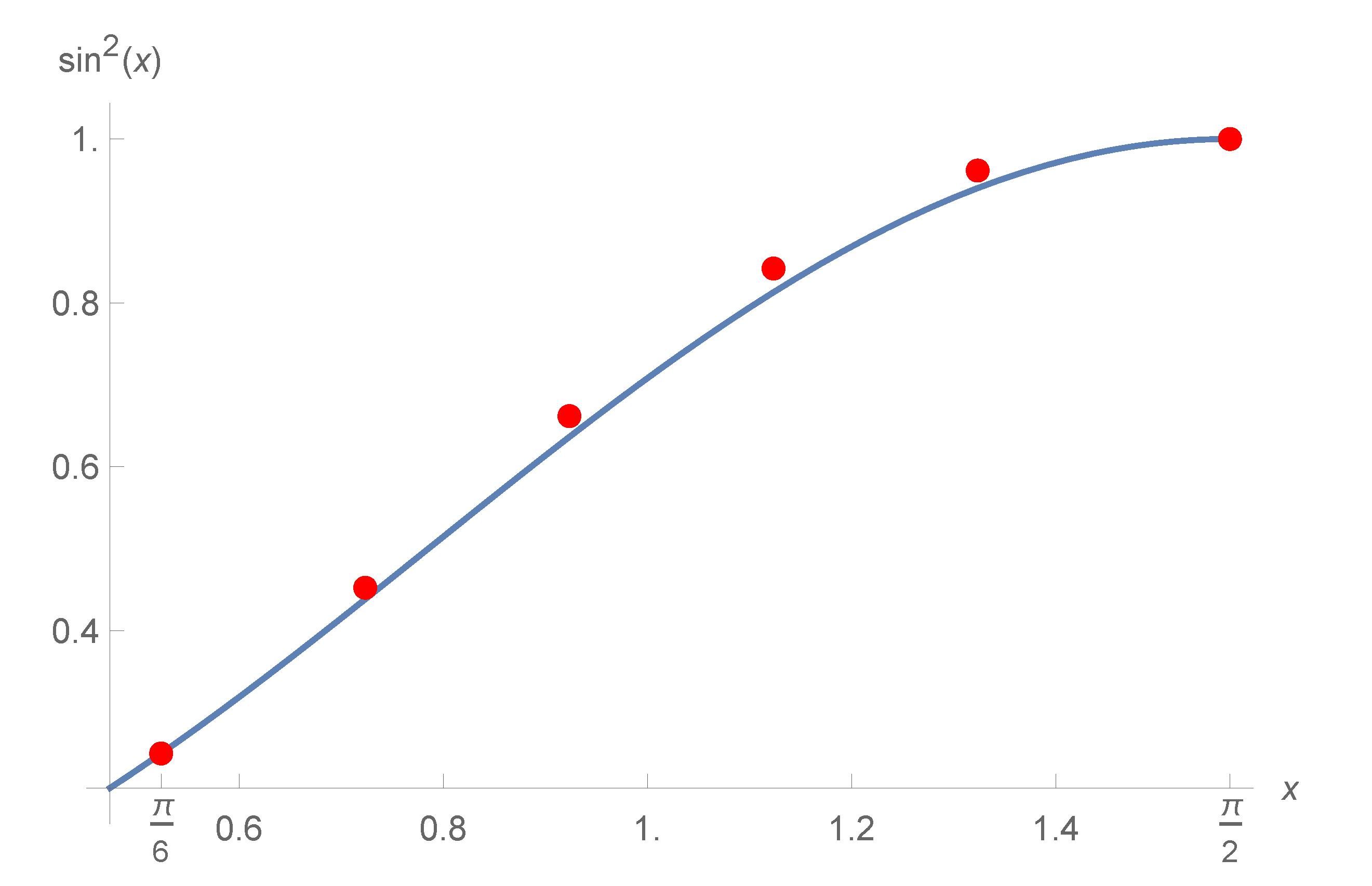
and Figure 5. It is seen that ACOC approaches up to 6, which is the theoretical order of convergence.

The errors $|{(sinx)}^2-y_i|$ for $1\le i\le 4)$ at the internal nodes are, respectively, given by:

$$\left(\begin{array}{cc}0.0045808024173838738376216319522,& 0.00731167760933327109201071704851,\\ 0.0073683157995758596940525729079,& 0.00474700015993753712029421111822.\end{array}\right)$$

As a remark, we should note that the numerical solution by the central finite-difference methods is accurate within the range of $\Delta y(x)=O(h^3)$ with $h=\frac{5\pi }{3N}=0.00918704$.

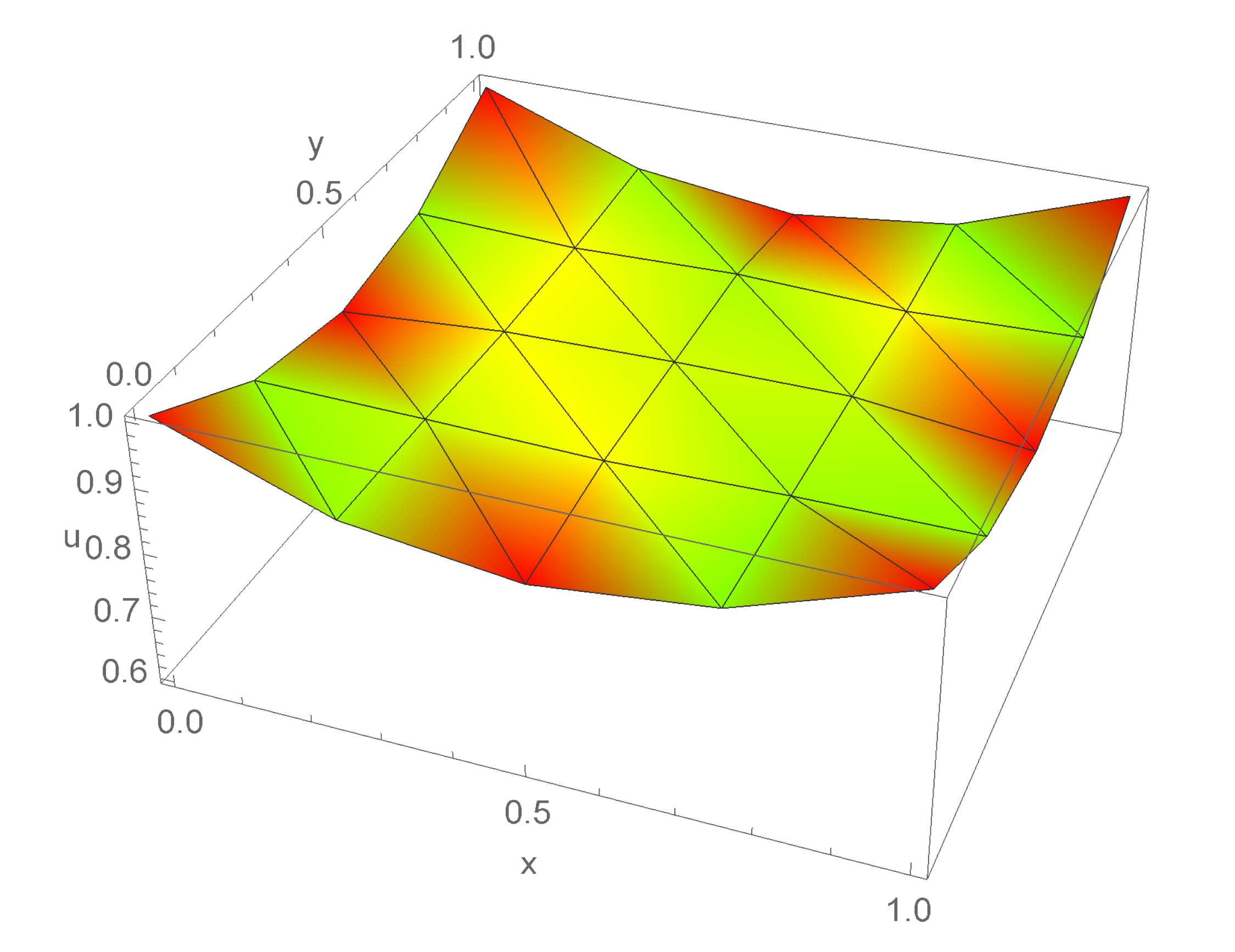
Test Example 3

A two-dimensional nonlinear reaction-diffusion equation for a concentration $u(x,t)$ of the substance under consideration in a bounded domain $\mathsf{\Omega }\subset {\mathbb{R}}^2$ with continuous boundary $\partial \mathsf{\Omega }$ is represented by an initial boundary value problem:

$$\left\{\begin{array}{c}{u}_t-d\Delta u=u(a-u)\mathrm{in}\mathsf{\Omega }\times (0,\infty ),\hfill \\ u=g\mathrm{on}\partial \mathsf{\Omega }\times (0,\infty ),\hfill \end{array}\right.$$

(43)

where $d>0$ is a diffusion coefficient, a is a positive constant, g is continuous on $\partial \mathsf{\Omega }$, and $\Delta$ is the Laplacian operator. For brevity of analysis, let $d=1$, $a=1$, and $\mathsf{\Omega }=[0,1]\times [0,1]$ (i.e., unit square region). We are interested in steady state solutions to (43), which lead us to elliptic partial differential equations with Dirichlet boundary conditions as follows:

$$\left\{\begin{array}{c}{u}_{xx}+u_{yy}=u(u-1)\mathrm{in}[0,1]\times [0,1],\hfill \\ u(x,0)=u(x,1)=\frac{x(x-1)}{2}+1,u(0,y)=u(1,y)=\frac{y(y-1)}{2}+1.\hfill \end{array}\right.$$

(44)

By using central divided differences with step $h=1/4$ in each component of the space vector, we discretize (44) into a nonlinear system of equations with 25 nodes, 9 of which constitute interior nodal variables $x_1,x_2,\cdots ,x_9$ in $\mathsf{\Omega }$, while the remaining 16 nodes are boundary nodes. As a result, we obtain a nonlinear algebraic vector equation $f:{\mathbb{R}}^9\to {\mathbb{R}}^9$ defined by:

$$f(x)=Ax+h^2\mathsf{\Psi }(x)-b=0,\mathrm{with}x={(x_1,x_2,\cdots ,x_9)}^T,$$

(45)

where $A=\left(\begin{array}{ccc}B& -I& 0\\ -I& B& -I\\ 0& -I& B\end{array}\right)$, $B=\left(\begin{array}{ccc}4-h^2& -1& 0\\ -1& 4-h^2& -1\\ 0& -1& 4-h^2\end{array}\right)$, I is the identity matrix of size $3\times 3$, $\mathsf{\Psi }(x)={(x_1^2,x_2^2,\cdots ,x_9^2)}^T$ and $b={(\frac{29}{16},\frac{7}{8},\frac{29}{16},\frac{7}{8},0,\frac{7}{8},\frac{29}{16},\frac{7}{8},\frac{29}{16})}^T$.

We solve (38) with an initial guess vector $x^{(0)}={(1,1,1,1,1,1,1,1,1)}^T$ by a typical method LK1, and find the results in

Table 7. Convergence results of Test Example 3.

$\mathit{\gamma }$	MT		k
			1	2	3
		$\left|\right|x^{(k+1)}-x^{(k)}\left|\right|$	2.230120 $\times {10}^{-1}$	6.736388 $\times {10}^{-13}$	4.536504 $\times {10}^{-82}$
	EM1	$\left|\right|f(x^{(k+1)})\left|\right|$	9.957324 $\times {10}^{-13}$	7.141684 $\times {10}^{-82}$	1.826912 $\times {10}^{-154}$
		ACOC	-	-	6.004539
		$\left|\right|x^{(k+1)}-x^{(k)}\left|\right|$	2.230120 $\times {10}^{-1}$	1.267438 $\times {10}^{-12}$	4.035285 $\times {10}^{-80}$
	EM2	$\left|\right|f(x^{(k+1)})\left|\right|$	1.767457 $\times {10}^{-12}$	6.182344 $\times {10}^{-80}$	3.498271 $\times {10}^{-154}$
		ACOC	-	-	6.002191
		$\left|\right|x^{(k+1)}-x^{(k)}\left|\right|$	2.230120 $\times {10}^{-1}$	2.766996 $\times {10}^{-12}$	1.050932 $\times {10}^{-77}$
	EM3	$\left|\right|f(x^{(k+1)})\left|\right|$	3.768017 $\times {10}^{-12}$	1.581912 $\times {10}^{-77}$	2.473651 $\times {10}^{-154}$
		ACOC	-	-	5.998396
		$\left|\right|x^{(k+1)}-x^{(k)}\left|\right|$	7.495256 $\times {10}^{-3}$	1.558196 $\times {10}^{-21}$	2.153197 $\times {10}^{-133}$
	EM4	$\left|\right|f(x^{(k+1)})\left|\right|$	2.256546 $\times {10}^{-21}$	3.262086 $\times {10}^{-133}$	1.826912 $\times {10}^{-154}$
		ACOC	-	-	5.987504
		$\left|\right|x^{(k+1)}-x^{(k)}\left|\right|$	2.230120 $\times {10}^{-1}$	3.364258$\times {10}^{-13}$	4.136278 $\times {10}^{-84}$
$2/3$	LK1	$\left|\right|f(x^{(k+1)})\left|\right|$	4.578823 $\times {10}^{-13}$	5.464893 $\times {10}^{-84}$	1.826912 $\times {10}^{-154}$
		ACOC	-	-	5.998447
		$\left|\right|x^{(k+1)}-x^{(k)}\left|\right|$	2.230120 $\times {10}^{-1}$	3.625463 $\times {10}^{-12}$	6.626067 $\times {10}^{-77}$
	LK2	$\left|\right|f(x^{(k+1)})\left|\right|$	4.879379 $\times {10}^{-12}$	9.868594 $\times {10}^{-77}$	3.498271 $\times {10}^{-154}$
		ACOC	-	-	6.000400
		$\left|\right|x^{(k+1)}-x^{(k)}\left|\right|$	2.230120 $\times {10}^{-1}$	1.690241 $\times {10}^{-12}$	3.277540 $\times {10}^{-79}$
	LK3	$\left|\right|f(x^{(k+1)})\left|\right|$	2.350565 $\times {10}^{-12}$	5.011579 $\times {10}^{-79}$	2.473651 $\times {10}^{-154}$
		ACOC	-	-	5.999111
		$\left|\right|x^{(k+1)}-x^{(k)}\left|\right|$	2.230120 $\times {10}^{-1}$	4.876737 $\times {10}^{-12}$	5.664655 $\times {10}^{-76}$
	LK4	$\left|\right|f(x^{(k+1)})\left|\right|$	6.554988 $\times {10}^{-12}$	8.425112 $\times {10}^{-76}$	4.775668 $\times {10}^{-154}$
		ACOC	-	-	5.997538
		$\left|\right|x^{(k+1)}-x^{(k)}\left|\right|$	2.230120 $\times {10}^{-1}$	1.633145 $\times {10}^{-11}$	2.761720 $\times {10}^{-72}$
	LK5	$\left|\right|f(x^{(k+1)})\left|\right|$	2.189664 $\times {10}^{-11}$	4.097352 $\times {10}^{-72}$	2.790655 $\times {10}^{-154}$
		ACOC	-	-	5.996055
		$\left|\right|x^{(k+1)}-x^{(k)}\left|\right|$	2.230120 $\times {10}^{-1}$	1.263880 $\times {10}^{-13}$	2.738954 $\times {10}^{-87}$
	EM5	$\left|\right|f(x^{(k+1)})\left|\right|$	3.328247 $\times {10}^{-13}$	5.839804 $\times {10}^{-87}$	2.473651 $\times {10}^{-154}$
		ACOC	-	-	6.015056
		$\left|\right|x^{(k+1)}-x^{(k)}\left|\right|$	2.230120 $\times {10}^{-1}$	1.440429 $\times {10}^{-12}$	3.815658 $\times {10}^{-75}$
	EM6	$\left|\right|f(x^{(k+1)})\left|\right|$	4.931396 $\times {10}^{-12}$	5.169287 $\times {10}^{-75}$	2.790655 $\times {10}^{-154}$
		ACOC	-	-	5.592300
		$\left|\right|x^{(k+1)}-x^{(k)}\left|\right|$	2.230120 $\times {10}^{-1}$	9.195040 $\times {10}^{-14}$	9.072776 $\times {10}^{-88}$
	EM7	$\left|\right|f(x^{(k+1)})\left|\right|$	3.009661 $\times {10}^{-13}$	1.315517 $\times {10}^{-87}$	2.473651 $\times {10}^{-154}$
		ACOC	-	-	5.975547
		$\left|\right|x^{(k+1)}-x^{(k)}\left|\right|$	2.230120 $\times {10}^{-1}$	1.540472 $\times {10}^{-12}$	4.642753 $\times {10}^{-74}$
1	LK6	$\left|\right|f(x^{(k+1)})\left|\right|$	5.029171 $\times {10}^{-12}$	6.674639 $\times {10}^{-74}$	2.790655 $\times {10}^{-154}$
		ACOC	-	-	5.503817
		$\left|\right|x^{(k+1)}-x^{(k)}\left|\right|$	2.230120 $\times {10}^{-1}$	2.772391 $\times {10}^{-13}$	2.131801 $\times {10}^{-78}$
	LK7	$\left|\right|f(x^{(k+1)})\left|\right|$	9.686043 $\times {10}^{-13}$	2.828895 $\times {10}^{-78}$	4.775668 $\times {10}^{-154}$
		ACOC	-	-	5.461376
		$\left|\right|x^{(k+1)}-x^{(k)}\left|\right|$	2.230120 $\times {10}^{-1}$	8.798181 $\times {10}^{-14}$	7.810164 $\times {10}^{-88}$
	LK8	$\left|\right|f(x^{(k+1)})\left|\right|$	2.973773 $\times {10}^{-13}$	1.085267 $\times {10}^{-87}$	2.473651 $\times {10}^{-154}$
		ACOC	-	-	5.970019
		$\left|\right|x^{(k+1)}-x^{(k)}\left|\right|$	2.230120 $\times {10}^{-1}$	1.521759 $\times {10}^{-11}$	4.464500 $\times {10}^{-75}$
	LK9	$\left|\right|f(x^{(k+1)})\left|\right|$	5.00431 $\times {10}^{-11}$	6.355336 $\times {10}^{-75}$	4.284490 $\times {10}^{-154}$
		ACOC	-	-	6.238981
		$\left|\right|x^{(k+1)}-x^{(k)}\left|\right|$	2.230120 $\times {10}^{-1}$	3.140371 $\times {10}^{-12}$	4.176009 $\times {10}^{-74}$
	LK10	$\left|\right|f(x^{(k+1)})\left|\right|$	7.346393 $\times {10}^{-12}$	5.641973 $\times {10}^{-74}$	2.473651 $\times {10}^{-154}$
		ACOC	-	-	5.693155

. It is evident that ACOC reaches up to 6, being the theoretical order of convergence. As can be seen in Table 7, the methods with $\gamma =2/3$ appear to converge more quickly and better than those with $\gamma =1$.

Interior 16 nodal values of the steady-state solution of $u(x,t)$ are illustrated with adjacent nodal points connected by straight lines in Figure 6.

Test Example 4

A d-dimensional nonlinear equation $f:{\mathbb{R}}^d\to {\mathbb{R}}^d$ with $d=max(4,n\in \mathbb{N})$ is given by:

$$0=x_i-cos(x_i-\sum _{j=1}^4{x}_j),i=1,2,\cdots ,d\in \mathbb{N}.$$

(46)

The above nonlinear system is described in [4]. Selecting $n=10$, we find $d=10$ and solve (46) in ${\mathbb{R}}^{10}$ with an initial guess vector $x^{(0)}={(0.75,0.75,\cdots ,0.75)}^T$ for the desired root $x={(0.5149332,0.5149332,\cdots ,0.5149332)}^T\in {\mathbb{R}}^{10}$ in

Table 8. Convergence results of Test Example 4.

$\mathit{\gamma }$	MT		k
			1	2	3
		$\left|\right|x^{(k+1)}-x^{(k)}\left|\right|$	7.433286 $\times {10}^{-1}$	1.760138 $\times {10}^{-5}$	1.064249 $\times {10}^{-32}$
	EM1	$\left|\right|f(x^{(k+1)})\left|\right|$	4.777837 $\times {10}^{-5}$	2.888862 $\times {10}^{-32}$	1.826912 $\times {10}^{-154}$
		ACOC	-	-	5.884275
		$\left|\right|x^{(k+1)}-x^{(k)}\left|\right|$	7.433279 $\times {10}^{-1}$	1.832336 $\times {10}^{-5}$	1.699619 $\times {10}^{-32}$
	EM2	$\left|\right|f(x^{(k+1)})\left|\right|$	4.973815 $\times {10}^{-5}$	4.613549 $\times {10}^{-32}$	2.358534 $\times {10}^{-154}$
		ACOC	-	-	5.866238
		$\left|\right|x^{(k+1)}-x^{(k)}\left|\right|$	7.060120 $\times {10}^{-1}$	2.066996 $\times {10}^{-5}$	1.050932 $\times {10}^{-32}$
	EM3	$\left|\right|f(x^{(k+1)})\left|\right|$	3.968813 $\times {10}^{-5}$	4.518912 $\times {10}^{-32}$	2.437651 $\times {10}^{-154}$
		ACOC	-	-	6.098760
		$\left|\right|x^{(k+1)}-x^{(k)}\left|\right|$	7.433270 $\times {10}^1$	1.925233 $\times {10}^{-5}$	2.905803 $\times {10}^{-32}$
	EM4	$\left|\right|f(x^{(k+1)})\left|\right|$	5.225983 $\times {10}^{-5}$	7.887687 $\times {10}^{-32}$	7.458340 $\times {10}^{-155}$
		ACOC	-	-	5.847611
		$\left|\right|x^{(k+1)}-x^{(k)}\left|\right|$	7.433299 $\times {10}^{-1}$	1.638128$\times {10}^{-5}$	3.979469 $\times {10}^{-33}$
$2/3$	LK1	$\left|\right|f(x^{(k+1)})\left|\right|$	4.446645 $\times {10}^{-5}$	1.080211 $\times {10}^{-32}$	8.204174 $\times {10}^{-154}$
		ACOC	-	-	5.929892
		$\left|\right|x^{(k+1)}-x^{(k)}\left|\right|$	7.433252 $\times {10}^{-1}$	2.100907 $\times {10}^{-5}$	6.997564 $\times {10}^{-32}$
	LK2	$\left|\right|f(x^{(k+1)})\left|\right|$	5.702845 $\times {10}^{-5}$	1.899461 $\times {10}^{-31}$	7.075603 $\times {10}^{-154}$
		ACOC	-	-	5.820793
		$\left|\right|x^{(k+1)}-x^{(k)}\left|\right|$	7.320120 $\times {10}^{-1}$	2.190241 $\times {10}^{-5}$	3.727540 $\times {10}^{-32}$
	LK3	$\left|\right|f(x^{(k+1)})\left|\right|$	7.536565 $\times {10}^{-5}$	5.115079 $\times {10}^{-31}$	7.743651 $\times {10}^{-154}$
		ACOC	-	-	5.917090
		$\left|\right|x^{(k+1)}-x^{(k)}\left|\right|$	6.901011 $\times {10}^{-1}$	3.076737 $\times {10}^{-5}$	4.664651 $\times {10}^{-32}$
	LK4	$\left|\right|f(x^{(k+1)})\left|\right|$	4.454988 $\times {10}^{-5}$	1.225112 $\times {10}^{-31}$	7.375668 $\times {10}^{-154}$
		ACOC	-	-	6.164184
		$\left|\right|x^{(k+1)}-x^{(k)}\left|\right|$	7.433217 $\times {10}^{-1}$	1.951033 $\times {10}^{-5}$	3.688441 $\times {10}^{-32}$
	LK5	$\left|\right|f(x^{(k+1)})\left|\right|$	6.653254 $\times {10}^{-5}$	1.001212 $\times {10}^{-31}$	1.826912 $\times {10}^{-154}$
		ACOC	-	-	5.833646
		$\left|\right|x^{(k+1)}-x^{(k)}\left|\right|$	6.230120 $\times {10}^{-1}$	1.263880 $\times {10}^{-5}$	7.738954 $\times {10}^{-32}$
	EM5	$\left|\right|f(x^{(k+1)})\left|\right|$	3.328247 $\times {10}^{-5}$	5.839804 $\times {10}^{-32}$	2.473651 $\times {10}^{-154}$
		ACOC	-	-	5.585807
		$\left|\right|x^{(k+1)}-x^{(k)}\left|\right|$	6.621130 $\times {10}^{-1}$	1.440429 $\times {10}^{-5}$	1.815658 $\times {10}^{-31}$
	EM6	$\left|\right|f(x^{(k+1)})\left|\right|$	4.931396 $\times {10}^{-5}$	5.169287 $\times {10}^{-31}$	2.790655 $\times {10}^{-154}$
		ACOC	-	-	5.554915
		$\left|\right|x^{(k+1)}-x^{(k)}\left|\right|$	5.930120 $\times {10}^{-1}$	1.395040 $\times {10}^{-5}$	1.072776 $\times {10}^{-31}$
	EM7	$\left|\right|f(x^{(k+1)})\left|\right|$	3.009661 $\times {10}^{-5}$	1.315517 $\times {10}^{-31}$	2.473651 $\times {10}^{-154}$
		ACOC	-	-	5.642046
		$\left|\right|x^{(k+1)}-x^{(k)}\left|\right|$	6.212301 $\times {10}^{-1}$	2.450274 $\times {10}^{-5}$	3.642573 $\times {10}^{-31}$
1	LK6	$\left|\right|f(x^{(k+1)})\left|\right|$	5.029171 $\times {10}^{-5}$	6.674639 $\times {10}^{-32}$	2.790655 $\times {10}^{-154}$
		ACOC	-	-	5.864574
		$\left|\right|x^{(k+1)}-x^{(k)}\left|\right|$	7.433602 $\times {10}^{-1}$	1.398344 $\times {10}^{-5}$	7.304552 $\times {10}^{-34}$
	LK7	$\left|\right|f(x^{(k+1)})\left|\right|$	3.795743 $\times {10}^{-5}$	1.982791 $\times {10}^{-33}$	7.420955 $\times {10}^{-154}$
		ACOC	-	-	5.984871
		$\left|\right|x^{(k+1)}-x^{(k)}\left|\right|$	6.692451 $\times {10}^{-1}$	2.819751 $\times {10}^{-5}$	5.180461 $\times {10}^{-32}$
	LK8	$\left|\right|f(x^{(k+1)})\left|\right|$	2.973773 $\times {10}^{-5}$	1.085267 $\times {10}^{-32}$	2.473651 $\times {10}^{-154}$
		ACOC	-	-	6.110527
		$\left|\right|x^{(k+1)}-x^{(k)}\left|\right|$	3.931569 $\times {10}^{-1}$	1.115921 $\times {10}^{-5}$	5.460045 $\times {10}^{-32}$
	LK9	$\left|\right|f(x^{(k+1)})\left|\right|$	5.00431 $\times {10}^{-5}$	6.355336 $\times {10}^{-32}$	4.284490 $\times {10}^{-154}$
		ACOC	-	-	5.786415
		$\left|\right|x^{(k+1)}-x^{(k)}\left|\right|$	7.433626 $\times {10}^{-1}$	1.633627 $\times {10}^{-5}$	1.381626 $\times {10}^{-34}$
	LK10	$\left|\right|f(x^{(k+1)})\left|\right|$	4.43440 $\times {10}^{-5}$	3.750370 $\times {10}^{-34}$	6.459112 $\times {10}^{-154}$
		ACOC	-	-	6.241405

. It is evident that ACOC reaches up to 6, being the theoretical order of convergence. As can be seen in Table 8, the methods with $\gamma =2/3$ appear to converge more quickly and better than those with $\gamma =1$.

Computational Efficiency

The computational efficiency of an iterative method is defined by an efficiency index $E={\rho }^{1/d}$ [30], with $\rho$ as the order of convergence and d as the number of functional evaluations per iteration. We require n scalar functions for each f and $n^2$ for each $f^{\prime }$. The concept of the efficiency index E applied to a nonlinear system of vector equations has been extended to treat the concept of computational efficiency by using $CE={\rho }^{1/(d+op)}$ [4], where $op$ is the number of operations associated with products and quotients. Suppose that n is the size of the matrix needed in the nonlinear system of vector equations. Matrix inversion requires $\frac{n^3-n}{3}$ product-quotient operations and $LU$-decomposition technique for solving linear systems requires $n^2$ product-quotient operations, including the $n^2$ product-quotient operations related to matrix multiplication by a vector. Note that each method treated here follows the three set of linear systems (1) and has one matrix inverse $f^{\prime }{(x_n)}^{-1}$. Consequently, the number of functional evaluations plus product-quotient operations $d+op$ becomes $2n+2n^2+\frac{n^3-n}{3}+6n^2=\frac{n^3+18n^2+5n}{3}$, which gives us the computational efficiency $CE=6^{\frac{3}{n^3+18n^2+5n}}$ for each listed method.

Many real-life application problems include ones related to: interval arithmetic benchmark, neurophysiology, chemical equilibrium, kinematic application, combustion application, and economics modeling, whose studies are described in [31]. The methods used therein are based on second-order Newton-like approach which may be more efficient in real-life problems in terms of speed and computational cost. On the other hand, our proposed family of sixth-order methods (1) is much more accurate than Newton-like methods, but has more complexities owing to the high-order formulation and require more CPU time to get the desired solution.

One certainly has to acknowledge that determining a better method than the other one should be avoided through solving a function with a randomly chosen initial guess vector and comparing the number of convergent iterations.

6. Conclusions

A family of Jarratt-like iterative methods for scalar and vector equations is developed and its convergence properties are theoretically established through Theorems 1 and 2. Computational aspects applied to various test equations agree well with the convergence behavior claimed in the theory developed. Global convergence behavior of the listed methods is illustrated for typical polynomials based upon their basins of attraction. The basins of attraction suggest selecting members of the iterative methods (1) give better convergence.

We will focus our future study on extending the current approach with different weight functions to the development of higher-order iterative root-finders.