Parameter Combination Framework for the Differential Evolution Algorithm

Abstract

The differential evolution (DE) algorithm is a popular and efficient evolutionary algorithm that can be used for single objective real-parameter optimization. Its performance is greatly affected by its parameters. Generally, parameter control strategies involve determining the most suitable value for the current state; there is only a little research on parameter combination and parameter distribution which is also useful for improving algorithm performance. This paper proposes an idea to use parameter region division and parameter strategy combination to flexibly adjust the parameter distribution. Based on the idea, a group-based two-level parameter combination framework is designed to support various modes of parameter combination, and enrich the parameter distribution characteristics. Under this framework, two customized parameter combination strategies are given for a single-operation DE algorithm and a multi-operation DE algorithm. The experiments verify the effectiveness of the two strategies and it also illustrates the meaning of the framework.

1. Introduction

Differential evolution (DE) is a simple and efficient evolutionary algorithm that is used primarily for real-parameter global optimization [1]. It has been successfully applied to many real-world problems [2,3,4,5]; however, the performance of DE algorithms greatly depends on parameter settings, especially in complex optimization problems. It is therefore important to study parameter control strategies for DE algorithms.

Parameters of population-based intelligent optimization algorithms can be divided into three categories: (1) operation-related parameters such as scale factor (F) and crossover probability (CR), which are used by search operations in classical DE; (2) population size (NP) and related parameters generated by strategies for dynamically adjusting the population; and (3) high-level strategy parameters: some algorithms use multi-operation, multi-strategy, or multi-population mechanisms, and may introduce new parameters. A number of parameter strategies have been proposed [6,7,8]. The first category of parameters has a large influence on the algorithm and has always been the focus of parameter control strategy research. In recent years, the second category of parameters has been gradually paid attention to. The third category of parameters is related to specific high-level strategies and has no universal significance.

Different categories employ diverse methods and technologies. Within a category, parameter control strategies also vary and lead to distinct effects for specific problems. Current parameter control strategy research focuses mostly on searching for the most suitable parameter values for the current problem, process, stage, or individual. The methods employed by parameter control strategies may be deterministic rules or adaptive strategies. There are two problems involved in these methods: one is the way to define the concept of suitable parameter values, and the other is how to set the parameter values. For example, some deterministic strategies believe that in the early stage of evolution, the search process should concentrate on exploration, thus larger F and CR are suitable parameter value; while in the later stage, the algorithm should focus on exploitation, thus smaller F and CR may be more suitable. The corresponding methods have been proposed by some studies such as decreasing the parameter value according to the generation with linear functions or nonlinear functions [9,10]. Some adaptive strategies consider that the parameter values that make the individual evolution successful are suitable values, and the corresponding parameter control strategies has been proposed in some researches, such as setting parameter values through comparing the success rate of different parameter values [11,12], statistical successful parameter distribution [13,14,15,16,17,18,19,20], or retain successful parameter values [21,22].

There are also a few studies concentrated on exploring the effects of parameter combination. Parameter combination can be the combination of the values of multiple parameters of an algorithm. Some studies discuss the effect of different value combination of F and CR for DE, and some parameter control strategies try to reach the best combination value for F and CR [22]. Some recent studies considered the three parameter F, CR, and NP simultaneously [12,23]. In [24], the authors think that the parameters values space could be decomposed in three regions for different convergence type, however, they also stated that such a decomposition is difficult to be obtained. The authors proposed a parameter control strategy to keep the parameter values in the good convergence region. In addition to the combination of multiple parameters, the combination of multiple parameter values for one parameter in the population is a different idea. Parameter distribution is a complex combination state of this idea that the parameter values of the entire population present some distribution characteristics when the parameter control strategy is an individual-level strategy. In [25], for each of the target vectors, the value of F is switched between 0.5 and 2 in a uniformly randomized way, and the Cr value is also selected between 0 and 1. So for the population, the values of F and CR are combined by two values. The study of parameter combinations can also be extended to include the combination of parameter strategies, and combining parameter strategies with algorithm operations. In this paper, we pay great interest in the parameter distribution of the population and the combination of parameter distribution with different algorithm operations.

Through the experiments, we believe that the parameter combination (parameter distribution) has an impact on the algorithm performance, and designing proper parameter combination mode (parameter distribution characteristic) can improve the performance of the algorithm. Therefore, this paper proposes an idea as parameter region division and parameter strategy combination to support adjusting parameter distribution, while the idea still supports the traditional purpose of finding suitable parameter values. Based on the idea, we design a two-level parameter combination framework to flexibly support various modes of parameter combination. Then two parameter combination strategies are customized for DE under this framework. Our experiments verify the effectiveness of the two strategies and they also illustrate the meaning of the framework.

The remainder of this paper is organized as follows. Section 2 introduces the classic DE algorithm and related works on parameter control strategies. Section 3 discusses the effect of parameter distribution on DE algorithm. Section 4 introduces the proposed idea and the design of two-level parameter combination framework. Section 5 customize two parameter combination strategies, and Section 6 reports the experimental results and analysis. Finally, Section 7 presents the conclusions and proposals for future research.

2. Related Works

2.1. Classical Differential Evolution

Differential evolution (DE) is a population-based heuristic random search algorithm. It has three steps in each generation of evolution: mutation, crossover, and selection [1].

The population can be described as P_g = {x_1,g, x_2,g, …, x_NP,g}, where g is the current generation of the evolution process, and NP is the population size. X_i,g = {x_1,i,g, x_2,i,g, …, x_D,i,g} is an individual vector, where D represents the dimension size of the solution space. The population is initialized uniformly, after which DE enters the iterative evolutionary process until the termination condition.

(1) Mutation step: each individual in the population as a target vector generates a corresponding mutation vector through the mutation strategy. There are many variants of the mutation strategy. The naming convention is DE/x/y, where x is the selection method of the base vector and y is the number of difference vectors. The mutation strategy of classical DE is named DE/rand/1 as follows:

$$v_{i,g}=x_{r1,g}+F\cdot (x_{r2,g}-x_{r3,g})$$

(1)

where x_i,g is the target individual, x_r1,g, x_r2,g, x_r3,g, x_r4,g, and x_r5,g are random individuals selected from the population, which differ from one other and from x_i,g. x_rb,g is the best individual in the current generation, v_i is the generated mutation vector, and F is the scale factor parameter.

(2) Crossover step: the mutation vector v_i and target vector x_i exchange internal components to generate candidate vector u_i. There are generally two methods for crossover operations: binomial crossover and exponential crossover. Binomial crossover is a commonly used method, and its equation is as follows:

$$u_{i,g}=u_{j,i,g}=\{\begin{array}{cc}{v}_{j,i,g}\hfill & \hfill \mathrm{if}(ran{d}_j(0,1)\le CR\mathrm{or}j=j_{rand})\\ x_{j,i,g}\hfill & \hfill \mathrm{otherwise}\end{array}$$

(2)

where CR is the crossover probability parameter, u_i is the trail vector, and j is one of the dimensions of the vector (j = 1, 2, … , D).

(3) Selection step: this step determines which vectors enter the next generation. The DE algorithm uses binary greedy selection between the target vector xi and trail vector u_i. The equation is as follows:

$$x_{i,g+1}=\{\begin{array}{cc}{u}_{i,g}\hfill & \hfill f(u_{i,g})\le f(x_{i,g})\\ x_{i,g}\hfill & \hfill \mathrm{otherwise}\end{array}$$

(3)

2.2. Related Works on Parameter Control Strategy for DE

The first category of parameters is related to operations performed by the individual; parameter control strategies can thus be population-level strategies or individual-level strategies. With a population-level parameter control strategy, the entire population shares the same parameter values. With an individual-level parameter control strategy, each individual has their own parameter value; thus, individuals in the population have different behavioral characteristics.

Research on the first parameter category mainly concerns parameters F and CR. The methods adopted by the parameter control strategy include the following: using fixed value, using random value, changing value according to evolutionary generation, changing value according to individual fitness, changing value according to the population model, test feedback based on statistics, and test feedback based on the single individual evaluation.

The parameter control studies of the DE algorithm begin with the random mechanism. This is an individual-level mechanism, and each individual is assigned a random parameter value. The values of the entire population may have distribution characteristics such as uniform distribution [9], normal distribution [26], or Cauchy distribution. Several studies discretized the parameter domain into a value set and randomly extracted from it. The set may be for single parameter [27] or for a combination of several parameters [28].

The strategy of changing parameter values according to evolutionary generation is generally a part of the population-level strategy. The parameter value is set by different functions (or rules) of generation such as linear functions [9] or nonlinear functions [10].

Parameter strategies that vary by individual fitness are individual-level strategies, where parameter values differ for each individual according to their fitness. The authors of [29] consider that the parameter values for individuals with good fitness should be smaller, and vice versa. In [30], the F value is set with the same idea as [29], however, the CR is adjusted according to the fitness of the donor vector, which is not a general strategy. In [31] the fitness of donor vector is also be used to adjust the parameter value.

Strategies for changing values according to the population model are primarily population-level strategies. The model is constructed according to the entire population and uses the deterministic rules or adaptive method to adjust parameter values for the population. A fuzzy adaptive differential evolution algorithm (FADE) [32] has designed a fuzzy model to adapt parameters F and CR, and in [33], a two-level parameter adaptation strategy is proposed. The first level involves adjusting the population parameters according to the population model, and in the second level, the individual parameters are adjusted according to the individual’s fitness based on the population parameter values.

Test feedback strategies based on statistics are primarily adaptive individual-level strategies. An adaptive DE algorithm named JADE [13] uses the results of the last generation to count the mean of the parameter (F and CR) of all good individuals by the Lehmer mean, which is used to guide the distribution of parameter values for the next generation. The values of the individual parameters are assigned according to normal distribution for CR and Cauchy distribution for F based on the mean. Success History based DE (SHADE) [14] improved the JADE strategy by (1) proposing a weighted method for the mean formula, and (2) proposing a history list for storing the successful mean of several recent generations. Many algorithms have used JADE or SHADE parameter strategy directly or with improvement [15,16,17,18,19,20]. References [11,12] discretize the parameter domain and use the results of the previous generation or a period to count the success rate of each discrete parameter value. They then use the success rate to modify the selection probability of each discrete parameter value to guide the individual’s parameter allocation.

Test feedback strategies based on the individual evaluation are considered individual-level strategies. Each individual is evaluated and the parameter value of the individual is adjusted independently. A typical strategy is proposed by jDE [21]. An algorithm of ensemble of mutation strategies and parameters in DE ( EPSDE) [22] presents a discretized version of this type of parameter strategy. The concept behind these methods is that good parameter values survive and propagate, while poor ones are discarded.

There are also some studies use a metaheuristic optimization algorithm to optimize the parameters of DE, such as [34,35].

In addition to F and CR, several studies have introduced other parameters in the first category. In JADE, a new mutation operation is proposed [13], and a new parameter p is introduced. JADE uses a fixed value for p, but in jSO [20], p is changed according to generation. Some studies utilize the neighborhood relationship to select parents; neighbor size may thus be a new parameter [36,37,38]. Reference [38] uses four neighborhood topologies, where the related parameters are fixed.

The relationship between DE performance and the second category of parameters has not been deeply studied. Some studies relate NP to the problem dimension D, but the advices on the value of NP differ greatly from 1D to 40D [39]. Some studies set NP as fixed and independent of D; 50 and 100 are primarily used in many DE variants [13,14,21]. Recently, several strategies with a variable population size have been proposed, and the concept of a gradual decrease in population size is referenced in some studies. dynNP-DE [40] reduces the population size by half for every 25% of function evaluations. L-SHADE provides a linear population size reduction strategy [18] that changes the NP every generation. Another proposal that changes the NP adaptively according to improvements to the best solution is adopted in several studies, which alternately increase or decrease the NP [41,42].

The third category of parameters does not share common parameters; different high-level strategies may use different parameters [15,17,22,26,27].

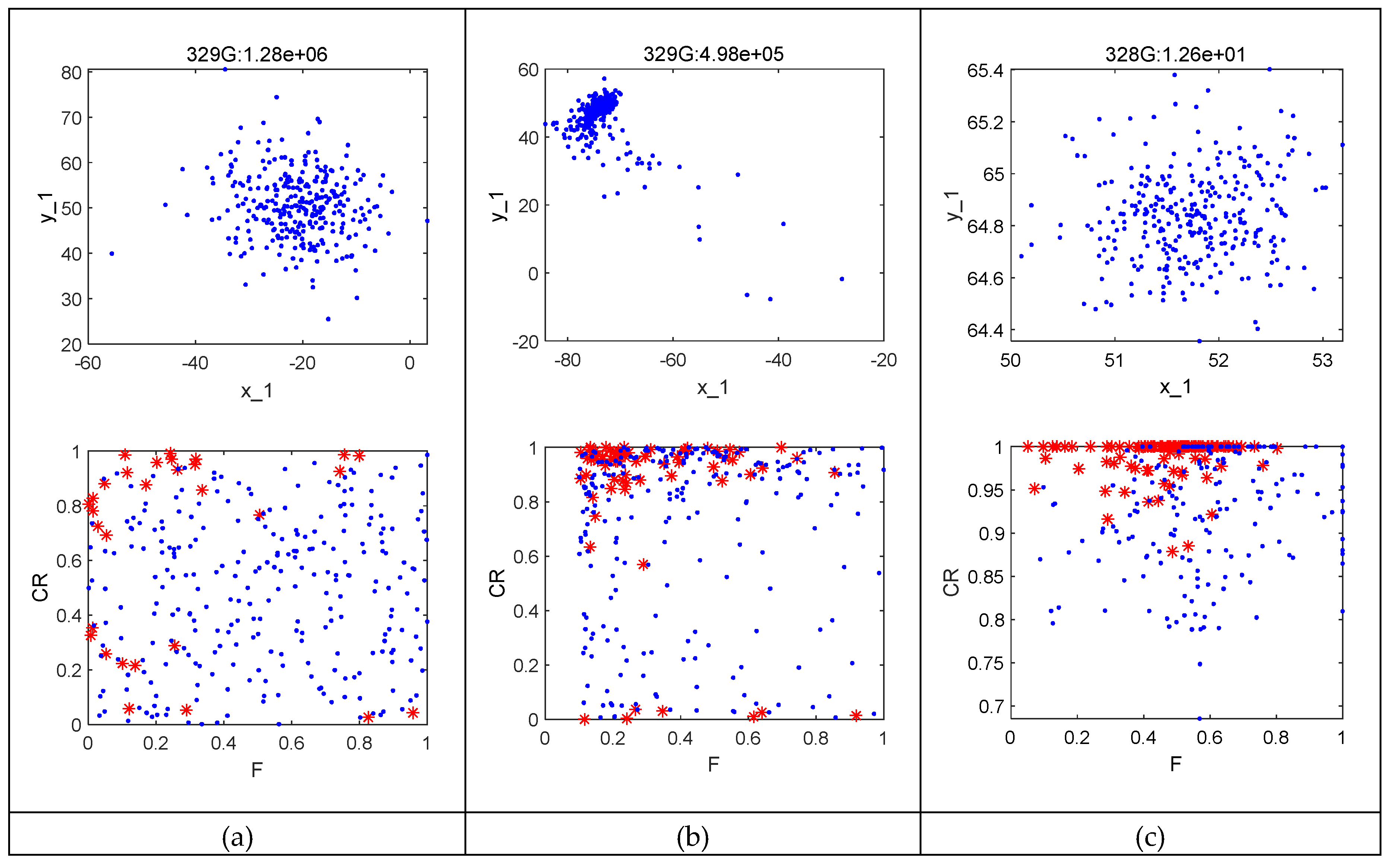
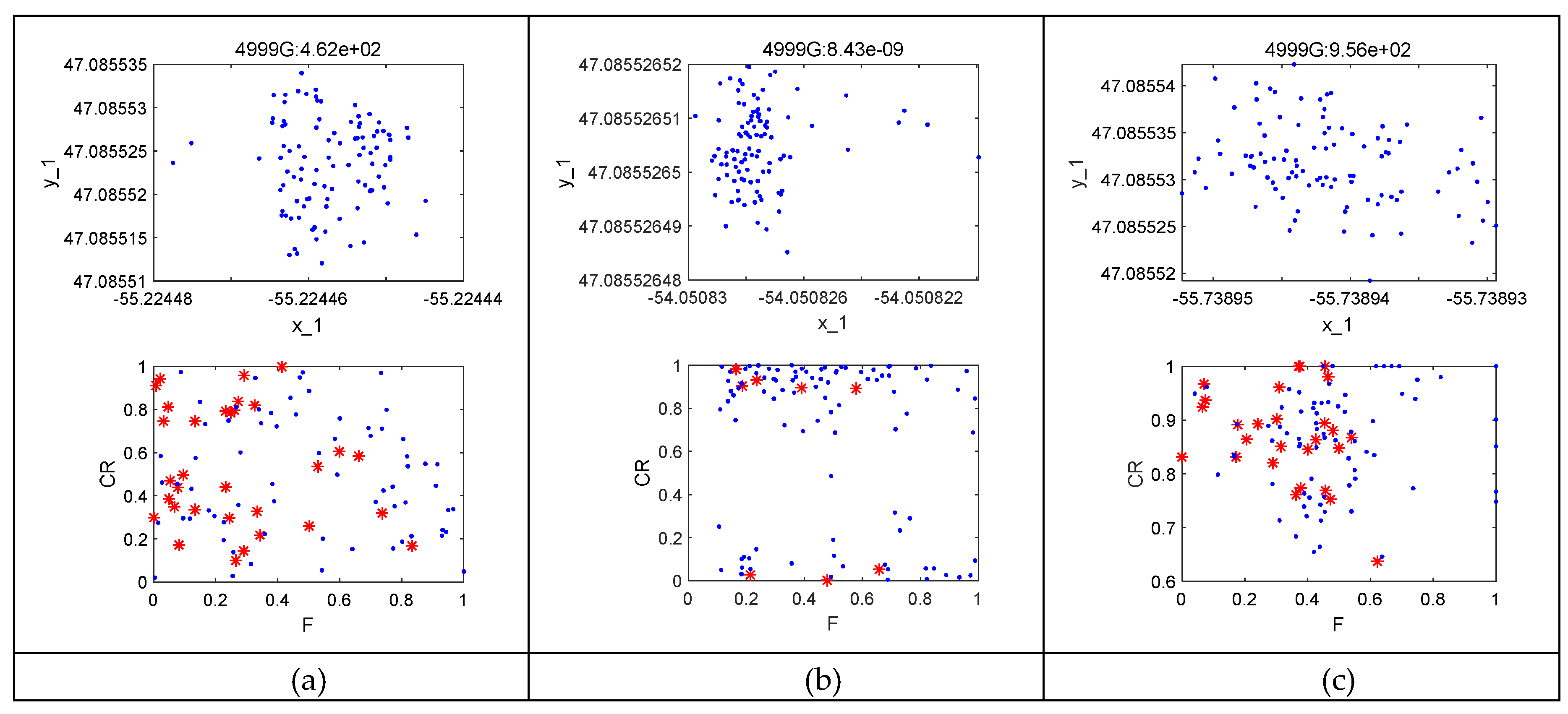
3. The Effect of Parameter Distribution on DE Algorithm

For the population-level parameter control strategy, all individuals share the same parameter value, and the parameter value may vary during the evolutionary process, making the parameter value more suitable for the current evolutionary state of the population. For individual-level parameter control strategy, each individual has its own parameters, and thus the parameter values of the entire population present some distribution characteristics in the parameter space. However, the current individual-level parameter strategies still aim to find the suitable parameter values, such as JADE [13], SHADE [13], and jDE [21], the focus of the current study is not on the parameter combination or distribution. There are few studies specifically focusing on the effects of parameter distribution. In this section, we study the influence of parameter control strategy on parameter distribution and the influence of parameter distribution on algorithm performance by experiments.

We chose three individual-level parameter control strategies: the jDE parameter strategy [21], SHADE parameter strategy [13], and a random parameter strategy. The test functions were extracted from the CEC2014 benchmark test function [43] with the maximum number of evaluations 10,000 × D. The optimization effect is relevant to operations, operation-related parameters (F, CR), population size (NP), and test functions. For comparison, we let the parameter strategy change while the others factors remained the same.

The first test was for function f1(30D), and the NP was set to 300. We adopted the DE/current-to-pbest/1 [13] mutation operation, binomial crossover operation and the other operations were the same as the classic DE. We observed the running distribution state of all individuals and the corresponding parameter values and intercepted the map, as shown in Figure 1. In each subfigure, the graph above displays the individual distribution, and the graph below displays the corresponding parameter distribution. The population’s individual distribution uses the plane of the first and second dimensions of the individual, while the parameter distribution uses the parameter plane on F and CR. The numbers at the top of each subfigure represent the generation and current optimal value, and red stars represent successful parameters. From Figure 1, the distribution characteristics of the three strategies can be seen, as described below.

• The parameters of the random parameter strategy are evenly distributed regardless of the evolutionary state. There are evidently many parameter values that are not beneficial to evolution that affect the efficiency of the strategy.
• The population parameter distribution of the jDE parameter strategy gradually coincides with the distribution of successful parameter values along with the evolutionary process; however, the process is slower.
• The parameter distribution of the SHADE parameter strategy spreads around a center point, and the distribution is shifted by the difference between the mean of the successful parameter-values and the entire parameter-values. The SHADE parameter strategy enhances a part of the distribution of successful parameter values.

The SHADE strategy is superior for f1, while the jDE strategy is prone to converge for many small F values in the distribution, which impacts exploration. The random strategy displays the worst results for many invalid parameter values. It is evident that parameter distribution affects algorithm performance.

The second test involved a mutation strategy of DE/rand/1 and a test function of f2 on 50D. The NP was set to 100. The other settings are the same as the first test. The intercepted running state is shown in Figure 2, where it can be seen that the distribution characteristics of the three parameter strategies have not changed.

However, an entirely different result appears: the SHADE strategy that performed well in the first test fell into a premature convergence. Premature convergence is identified by the state that the individual distribution is converged in a wrong region for a long period. As in individual distribution subgraph of Figure 2c, the first dimension is converged to 1e-5 precision, but the offset between the convergence location and the optimal value location is 1e1 precision, and has not improved in many generations. However, the jDE strategy that was apt to converge in the first test found the correct region and yielded optimal result.

These two tests demonstrate that operation is related to parameter strategy. For the DE/rand/1 operation, the jDE strategy performs better than the SHADE strategy on test function f2, while for the DE/current-to-pbest/1 operation, the jDE strategy performs more poorly than SHADE on test function f1. The SHADE strategy, which is generally an excellent parameter strategy, is not ideal for all operations. Thus, different combination mode of operation and parameter strategy should produce different search characteristics and may be suitable for different problems.

Since jDE and SHADE parameter strategy produce very different parameter distribution characteristics, we consider that the difference of algorithm performance in the tests is due to the distribution of the two parameters F and CR. We designed further experiments based on the second test to verify whether changing the parameter distribution would improve the performance of the algorithm. The algorithm is identical with the second test except the parameter strategy, and the test function is still f2. For the parameter strategy we designed several different parameter region combinations. For the sake of discussion, we divided the domain of F and CR into two subdomains: large value [0.5, 1] and small value [0, 0.5]. Then, the plane of F and CR formed four regions, as shown in Figure 3. The experiment on all types of region combination patterns was performed, and the results are shown in

Table 1. Results for all region combination patterns.

Region Combination Pattern	Result	Premature Convergence
(1)	7.6e+02	N
(2)	1.0e+04	N
(3)	5.2e+03	Y
(4)	1.4e+03	Y
(1,4)	3.1e-03	N
(1,2)	6.0e+00	N
(1,3)	8.4e+02	Y
(2,3)	6.4e+02	Y
(2,4)	4.1e+03	Y
(3,4)	7.1e+02	Y
(1,2,4)	1.3e-01	N
(1,3,4)	2.0e+03	Y
(1,2,3)	3.5e+02	N
(2,3,4)	4.3e+03	Y
(1,2,3,4)	2.9e+02	N

. For each combination, the subregions are assigned the same number of individuals. Each region uses the SHADE parameter strategy. Premature convergence is identified as described in the second test.

Initial domain is including region 1-4, but without division and combination. From Table 1, we can conclude that different regions have different effects and that combination patterns can affect the distribution of parameters and strengthen or weaken the effect. For example, with the region 4, premature convergence occurs, but when combined with the region 1, the result is superior than those for either region individually. The proper distribution or combination of parameter values can thus be useful for algorithms.

From the experiments, we acquire several conclusions:

(1) different parameter control strategies may produce different parameter distribution.

(2) the parameter distribution will influence the performance of the algorithm.

(3) the parameter strategy is related to the operation adopted by DE variants.

(4) adjusting the parameter distribution makes sense for improving the algorithm.

The distribution of parameters cannot, however, be flexibly controlled by a simple formula or a single strategy. For example, the jDE parameter strategy treats all successful parameter values equally, the SHADE strategy has a limitation on the combination of parameter values which cannot support maximal and minimum values simultaneously. Thus, we have designed a flexible parameter combination framework that can support multiple forms of parameter combination and customize the parameter distribution.

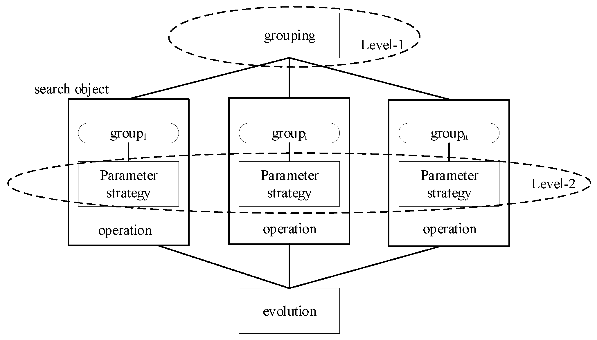
4. Two-Level Parameter Combination Framework

We proposed an idea as parameter region division and parameter strategy combination. The method is to divide the domain of the related parameters into several subdomains. Thus, the feasible parameter space forms multiple regions. The parameter distribution can be customized by choosing one or more regions. These regions can be overlapped or disconnected, and some regions can be removed from the feasible parameter space. In each region, the parameter strategy can be chosen, which produces the specific parameter distribution within the region. The parameter strategy can be an adaptive strategy, then the merits of the traditional parameter strategy of finding suitable parameter value within the region can still be remained in our idea. The combination of regions instructs the distribution scope; while the combination of parameter strategy instructs the distribution details. When the region degenerates into a point, the method turns to a simple parameter value combination method.

We designed a group-based two-level parameter combination scheme to support the idea. Each group correspondents to a parameter strategy including region and parameter control method. The scheme has a two-level architecture as described in Figure 4. Level-2 adjusts the parameter distribution with the basic parameter strategy in the specific region, and level-1 combines or adjusts the basic parameter strategies or regions by population grouping. The individual number of each group represents the ratio of each region. Therefore, adjusting the group size can lead to the change of parameter density in each region.

The scheme is implemented as a general framework. For the traditional algorithm structure, parameter strategy and evolutionary operation are coupled together, thus the change and combination of the parameter strategies are very difficult. Whereas a framework structure can support the parameter value combination, parameter region combination, parameter strategy combination, parameter strategy, and evolutionary operation combination, and can flexibly customize different parameter combination strategy.

4.1. Search Object with Specific Parameter Region and Strategy

A concept of search object is defined to represent an algorithm based on a specific parameter strategy design and performed by an individual group. A search object includes information and search action.

The information of the search object STRinfo is a five-tuple: STRinfo = (opstrategy, pastrategies, group, environment, model), where opstrategy represents the evolutionary operation, pastrategies is a set of parameter strategy (pastrategy) for different parameters of the operation, and pastrategy is a five-turple: pastrategy = (pa, type, num, domain, painfo). Here, pa is the parameters that the strategy deals with, type is the parameter strategy type, num is the strategy ID, domain is the parameter scope, painfo is the information for parameter strategy model. group is the group of individuals to perform the evolutionary operation: group = (size, indiset, character). Here, size is the group size, indiset is the individual set, and character is the characteristics of the set to instruct the grouping. environment is the environment of the searching group that generally represents the neighborhood scope, and model is the evaluation information of the current strategy.

The parameter strategy is designed as algorithm components such as jDE strategy, SHADE strategy, random strategy, and L-SHADE strategy for NP parameter and so on. The same type of strategies uses a uniform interface to facilitate combination with algorithm operation. The operation-related parameter strategy is divided into two phases. Phase 1 is used for collecting information and establishing the model, whereas phase 2 is used for assigning parameter values according to the model.

The action of the search object is described in Algorithm 1.

Algorithm 1. Execute search object algorithm.

Input: STRinfo Output: offspring set, STRinfo.model 1: According to the STRinfo.group, assign the individual set. 2: foreach parameter strategy in STRinfo.pastrategies 3:       Execute the parameter component with phase 2 to generate the parameter value set. 4: end foreach 5: Execute the operation (STRinfo.opstrategy) and return the offspring set. 6: Compute the objective of the offspring. 7: foreach parameter strategy in STRinfo.pastrategies 8:       Execute the parameter component with phase 1 to collect information and construct the parameter strategy model. 9: end foreach. 10: Collect the algorithm evaluation information to generate STRinfo.model.

4.2. Grouping for Search Object

During the search process, multiple search objects exist with different parameter strategy settings (STRinfo.pastrategies). Each search object represents an algorithm with specific parameter strategy and generates specific parameter distribution. The parameter distribution of entire population is the combination of multiple search objects. Therefore, the grouping is the first-level of distribution adjustment mechanism which can change the ratio and density of parameter distribution of each search object by changing group size. We design two grouping method in this section to adjust the group size: competition method and collaborative method. Let m represent the number of search objects. Dynamically divide the population into group set G at runtime, where group_i ∈ G. Let NP_i be the size of group_i. It is clear that NP₁ + NP₂ + … + NP_m = NP. Each group is assigned to a search object, and each search object shares information about the entire population. First, we define the evaluation model for the search object, and then define the method for computing NP_i.

4.2.1. Evaluation Model for Search Object

We define the vector STRinfo.model to describe the data that are to be collected for every generation: STRinfo.model = (s₁, s₂), where s₁ is designed as the success rate of the search object and s₂ is designed as the fitness improvement state. In every generation, for each search object so_i, we compute the success rate (SR_i) and the fitness improvement mean (FIM_i) as follows:

$$S{R}_i=\frac{count(S{I}_i)}{N{P}_i}$$

(4)

$$FI{M}_i=\frac{{\displaystyle {\sum }_{k=1}^{\left|S{I}_i\right|}\mathsf{\Delta }{f}_k}}{count(S{I}_i)}$$

(5)

$$\mathsf{\Delta }{f}_k=|f(u_{k,g})-f(x_{k,g})|$$

(6)

SI_i is the set of all successful individuals in STRinfo_i.group. We then convert SR_i and FIM_i to the ratio of all the search objects as PSR_i and PFIM_i:

$$PS{R}_i=\frac{S{R}_i}{{\displaystyle {\sum }_{j=1}^{m}S{R}_j}}$$

(7)

$$PFI{M}_i=\frac{FI{M}_i}{{\displaystyle {\sum }_{j=1}^{m}FI{M}_j}}$$

(8)

for each search object, we update v1 and v2 as follows:

$$STRinf{o}_i.model.s_1=c\cdot STRinf{o}_i.model.s_1+(1-c)*PFI{M}_i$$

(9)

$$STRinf{o}_i.model.s_2=c\cdot STRinf{o}_i.model.s_2+(1-c)*PS{R}_i$$

(10)

where c is set to 0.5. We then calculate the evaluation model for each search object as follows:

$$soStat{e}_i=w\cdot STRinf{o}_i.model.m_1+(1-w)\cdot STRinf{o}_i.model.m_2$$

(11)

where w is the linear increment from 0 to 0.5 by generation, and soState_i is the evaluation model for search object so_i.

4.2.2. Collaboration-Based Grouping Method

In collaboration mode, each search object has its own task and has the basic proportion (P_base,i) for group size. This means that the search object (so_i) has the basic individual numbers of NP*P_base,i. If the sum of all P_base,i (i = 1 … m) is less than 1, the remaining individuals are allocated to the search objects according to their model score. NP_i can thus be computed as follows:

$$N{P}_i=NP\cdot (P_{base,i}+{\delta }_i)$$

(12)

$${\delta }_i=(1-{\displaystyle {\sum }_{i=1}^m{P}_{base,i}})\cdot \frac{soStat{e}_i}{{\displaystyle {\sum }_{i=1}^{m}soStat{e}_i}}$$

(13)

4.2.3. Competition-Based Grouping Method

In competitive mode, better search objects are encouraged, and poorer objects transfer their resources to the better search objects according to their score, originating from the evaluation model. The soState of all search objects are sorted and the best set of search object is found, as shown in (14). The rest search objects reduce their group size ∆_i and add ∆_i to the best ones (15), (16) [44]. ∆_i is computed from the difference between the best search object and the i-th search object, as shown in (17) [44]. The rate is the reduction ratio, set to 0.05. The group size has a lower limit (P_min), and NP_i is no less than NP*P_min. We set P_min as 0.05 for large NP and 0.1 for small NP.

$$best=\left\{i|soStat{e}_i>avg(soState)\wedge \frac{soStat{e}_i-avg(soState)}{soStat{e}_{best}-avg(soState)}>0.5\mathrm{i}\in [1,m]\right\}$$

(14)

$$N{P}_i=\{\begin{array}{c}N{P}_i+\eta \mathrm{if}\mathrm{i}\in \mathrm{best}\\ N{P}_i-\mathsf{\Delta }i\mathrm{otherwise}\end{array}$$

(15)

$$\eta =\frac{{\displaystyle {\sum }_{i\notin best}{\mathsf{\Delta }}_i}}{\left|best\right|}$$

(16)

$${\mathsf{\Delta }}_i=N{P}_i\cdot rate\cdot \frac{soStat{e}_{best}-soStat{e}_i}{soStat{e}_{best}}\mathrm{i}\notin \mathrm{best}$$

(17)

4.3. The Algorithm of the Framework

The framework can customize different parameter combination mode. Based on some design principle for evolutionary algorithm, the algorithm can be designed by defining several search objects. The initial group size ratios (Igsr) for all search object, grouping strategy, regrouping interval (GroInt) should be decided. Furthermore, each search object should be designed includes evolutionary operation, all the algorithm parameters, and the parameter strategy and parameter domain for each parameter. The algorithm of the framework is described as Algorithm 2.

Algorithm 2. The algorithm of the framework.

1: Initialize the population. 2: Evaluate the individuals of the population 3: According to the design of search objects, create the runtime list of so with STRInfo. 4: while (not (termination condition)) 5:       if (the first generation) 6:         grouping the population according to the initial group size ratio (Igsr). 7:      else 8:         if t= =GroInt 9:           t = 0; 10:           execute grouping strategy (collaboration method or competition method) to adjust the group size of each search object. 11:           grouping the population and assign the group to search object(so). 12:         else 13:           t = t + 1; 14:         end if 15:      end if 16:       foreach soi in search object list 17:         execute soi, generate the offspring and STRInfo.model(Algorithm 1) 18:       end foreach 19:       compute the model score of each search object (soState) 20:      generate the next generation population according to population selection method. 21:       execute the parameter component for population adjusting if needed. 22: end while

5. Customizing Two Parameter Combination Strategies

In this section, we customize two specific parameter combination strategies by defining their search objects (STRInfo).

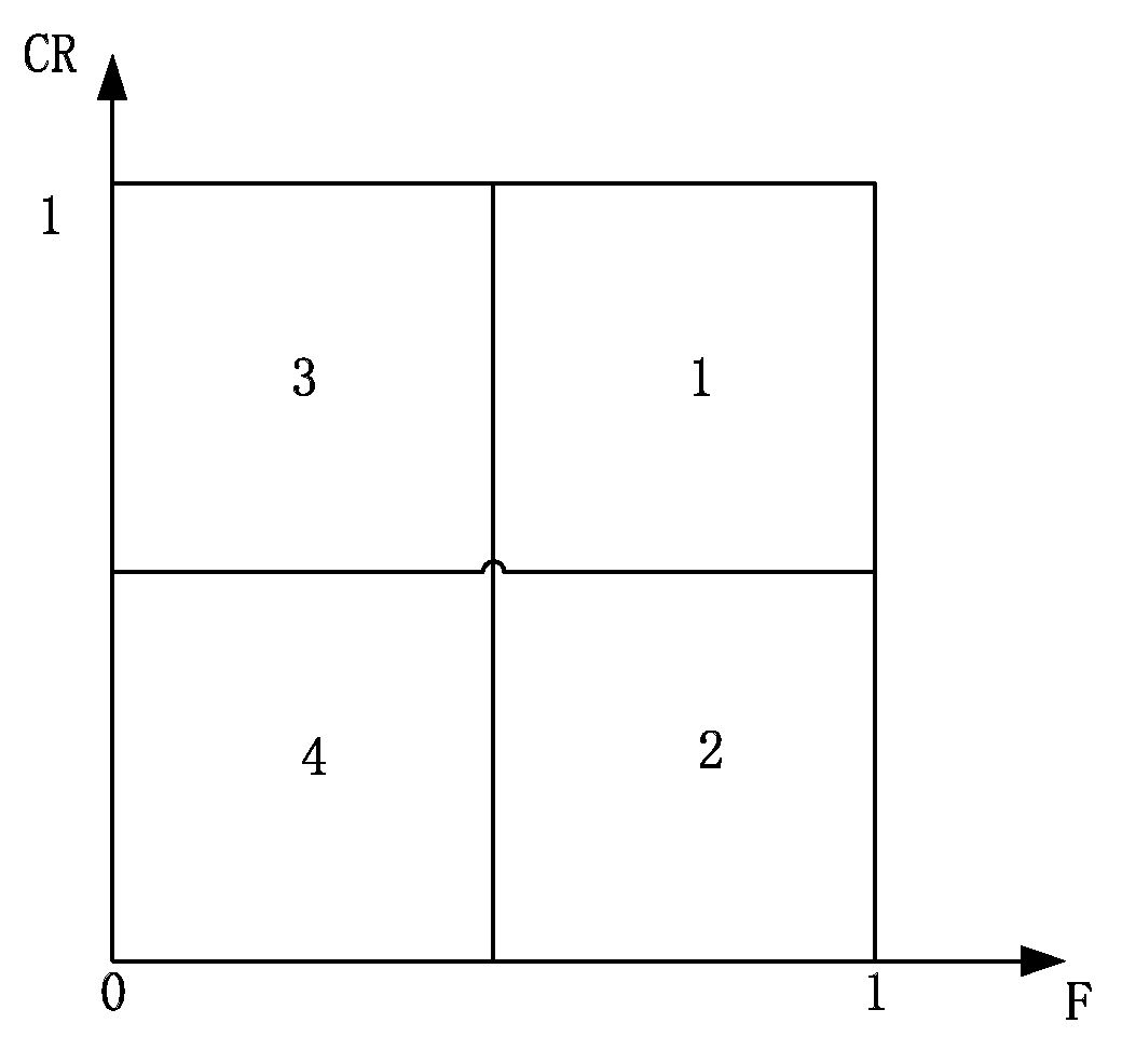
5.1. Combine Parameter Regions or Values for Single-Operation DE

This strategy we named PVCDE (Parameter Values Combination for DE) is designed for single-operation DE which means that the multiple search objects use the same evolutionary operation but with different parameter values (or regions). For the DE algorithm, we chose the mutation operation DE/current-to-pbest/1 proposed by the JADE algorithm, as follows:

$$v_i=x_i+F\cdot (x_{pbest}-x_i)+F\cdot (x_{r2}-x_{r1})$$

(18)

where x_pbest is an individual that is randomly selected from the top NP × p (p ∈ [0, 1]) sorted individuals in the current generation. x_r2 is a random individual in the population, and x_r1 is selected from the population and archive which contains the failed individuals from the selection step. The crossover strategy is binomial crossover, and the selection strategy is the same as the classic DE. The parameters include NP, F, CR, p, and archive-size. NP and archive-size are set as fixed values, and F, CR, and p are controlled by region combination (for F and CR) and value combination (for p) method.

In addition to the regions in Figure 3, we add two regions for F and CR.

• Region 5: F∈[0.1, 1], CR∈[0, 1]. This region consists of the entire range except for a very small F.
• Region 6: F∈[0, 1], CR∈[0, 1]. This region consists of the entire range.

We design three search objects. The first search object(so₁) is used for wide range search with large F, the second search object (so₂) is used for local search with small F and CR, and the third search object (so₃) performs the most favorable search for current state by adaptive parameter values in the entire parameter domain. With the overlapping of the parameter regions, the search focus can be changed by adjust the group size of each search object. All the search objects adopt the SHADE parameter control strategy for F and CR within their own region. SHADE parameter control strategy is an adaptive strategy and its parameter distribution characteristic is analyzed in Section 3.

We divide the evolutionary process into two stages. The first stage is an exploration stage, and the second stage is for exploitation. The design of search objects is showed in

Table 2. Parameter scheme of PVCDE.

Stage	Search Object	Parameter	Parameter Scope	Parameter Control Strategy
exploration	so1	F and CR	[0.5, 1] × [0.5, 1] (Region1)	SHADE
		p	0.1	fixed
	so2	F and CR	[0, 0.5] × [0, 0.5] (Region4)	SHADE
		p	0.1	fixed
	so3	F andCR	[0.1, 1] × [0, 1] (Region5)	SHADE
		p	0.5	fixed
exploitation	so1	F and CR	[0.5, 1] × [0, 1] (Region1∪Region2)	SHADE
		p	0.1	fixed
	so2	F and CR	[0, 0.5] × [0, 0.5] (Region4)	SHADE
		p	0.1	fixed
	so3	F and CR	[0, 1] × [0, 1] (Region6)	SHADE
		p	0.1	fixed

. In the initial stage, the search focus is exploration, thus we strengthen the region 1 by assigning larger group size to so₁, and weaken the region 3 and region 2 by assigning smaller group size to so₃ since its parameter distribution may move in the four regions. A so₂ with small group size achieves the purpose that region 4 cooperates with region 1. The grouping mode uses collaboration-based grouping method with predefined ratio of group size to NP. After the initial stage, the search enters the exploitation stage, thus, we strength so₃ and weaken so₁ and so₂ by adaptive competition-based grouping. A slight difference between the two stages can be seen in the Table 2. so₁ changes from region 1 to Region 1∪Region 2 in order to match a category of separable problem. so₃ varies from region 5 to region 6 to avoid minimal F value in the exploration stage. For parameter p, 0.1 is a suggested value in relevant papers, we combine 0.1 with 0.5 by so₃ in exploration stage for strengthen the exploration for so₃.

A little change for SHADE strategy also adopts in region 6. As in SHADE [20], the F_i for individual x_i is computed with Cauchy distribution as randc_i(M_F,ri, 0.1). When M_F,ri is less than 0.05, we use 1.1*M_F,ri to replace 0.1. F_i is still restricted in the scope [0, 1] as SHADE does, but we have more chances to get a small value (in the interval from 0 to M_F,ri) for F_i. The same method is used for CR, but the minimum value of CR_i is limited as 0.1/D.

5.2. Combine Different Parameter Strategies for Multi-Operation DE

This strategy we named PSCDE (Parameter Strategies Combination for DE) is designed for multi-operation DE which means that the multiple search objects use the different evolutionary operations. This method involves selecting the proper parameter strategy and region for evolutionary operation. We select two mutation operations, DE/current-to-pbest/1 and DE/rand/1, and construct two search objects. The crossover strategy is binomial crossover, and the selection strategy is the same as the classic DE. We match the DE/current-to-pbest/1 operation with SHADE parameter control strategy, and DE/rand/1 operation with jDE parameter strategy. The parameter distribution of jDE strategy has been analyzed in Section 3. We divide the evolutionary process into three stages with small changes to the parameter region or value as

Table 3. The parameter scheme of PSCDE.

Stage	Search Object	Parameter	Parameter Scope	Parameter Control Strategy
stage1	so1 (DE/rand/1)	F and CR	[0.1, 1] × [0, 1] (Region5)	jDE
	so2 (DE/current-to-pbest/1)	F and CR	[0.5, 1] × [0.5, 1] (Region1)	SHADE
		p	0.5	fixed
stage2	so1(DE/rand/1)	F and CR	[0.1, 1] × [0, 1] (Region5)	jDE
	so2 (DE/current-to-pbest/1)	F and CR	[0.1, 1] × [0, 1] (Region5)	SHADE
		p	0.1	fixed
stage3	so1(DE/rand/1)	F and CR	[0.1, 1] × [0, 1] (Region5)	jDE
	so2 (DE/current-to-pbest/1)	F and CR	[0, 1] × [0, 1] (Region6)	SHADE
		p	0.1	fixed

showed. The working mode between the two search objects is suitable for cooperation mode, because so₁ may fail when competing with so₂, however, it may be useful to escape a small range when the population falls into a local extremum. Therefore, we use collaboration-based grouping method with predefined group size ratio (Igsr).

6. Experiments and Discussion

In this section, we describe several experiments to test the proposed framework and methods. We performed an evaluation test on the CEC2014 Special Session on Real-Parameter Single Objective Optimization benchmark suite [40]. The CEC2014 benchmark set consists of 30 test functions. Functions F1–F3 are unimodal functions, F4–F16 are simple multimodal functions, F17–F22 are hybrid functions, and F23–F30 are composite functions. The search space is [−100, 100]^D. For every function, the maximum number of evaluations is 10,000 × D. According to the rules of CEC2014, the error between the best value found and the true optimal value is considered to be zero if it less than 1e-8. The algorithm in this paper is implemented with the MATLAB language and run in MATLAB R2018a.

We present the first test between SHADE and PVCDE. SHADE is a superior DE variant. PVCDE uses the same operations as SHADE, and the parameter strategy of PVCDE in Level-2 is also similar to that of SHADE. The only difference between them is the region division and combination. The comparison can thus test whether the method of region division and combination is valid. The algorithms settings are as follows:

• SHADE: The parameters for DE/current-to-pbest/1 operation are set to p = 0.1, archive-size = 2*NP, which is the same as that in the initial paper. The memory-size of the history list used by the parameter strategy is set as 6, referencing a previous study [24]. For parameter NP, we set the NP as 4D.
• PVCDE: The population size is set to NP = 5D for the purpose of grouping, with archive-size = 1.4*NP and memory-size = 6. The initial group size ratios (Igsr) are set as [8/10, 1/10, 1/10], and the basic proportions (P_base) of all search objects in phase 1 are set to [7/10, 1/10, 1/10], which emphasizes so₁. Every ten generations, the groups are reassigned, and the grouping method is random grouping. The switching conditions for stage 1 and 2 are 500 generations or the success rate of so₁ (STRinfo₁.model.s₁) being less than 0.01.

In the experiment comparing SHADE with PVCDE, all the functions with D = 30, 50, and 100 are tested 51 times. The test results on D = 30, 50, and 100 dimensions are shown in

Table 4. CEC 2014 function test for 30D, 50D, 100D on SHADE and PVCDE.

Fun	30D			50D			100D
	SHADE Mean (std)	PVCDE Mean (std)		SHADE Mean (std)	PVCDE Mean (std)		SHADE Mean (std)	PVCDE Mean (std)
1	1.50e+03 (2.35e+03)	3.68e-09 (2.63e-08)	−	6.42e+04 (3.19e+04)	1.31e+04 (1.03e+04)	−	4.03e+05 (1.35e+05)	3.25e+05 (9.86e+04)	−
2	0.00e+00 (0.00e+00)	0.00e+00 (0.00e+00)	≈	0.00e+00 (0.00e+00)	0.00e+00 (0.00e+00)	≈	8.00e-09 (1.60e-08)	0.00e+00 (0.00e+00)	−
3	0.00e+00 (0.00e+00)	0.00e+00 (0.00e+00)	≈	0.00e+00 (0.00e+00)	0.00e+00 (0.00e+00)	≈	2.54e-03 (3.77e-03)	2.57e-04 (1.83e-03)	−
4	0.00e+00 (0.00e+00)	0.00e+00 (0.00e+00)	≈	2.52e+01 (3.72e+01)	4.49e+01 (4.82e+01)	≈	1.26e+02 (4.50e+01)	1.71e+02 (3.06e+01)	+
5	2.01e+01 (5.54e-02)	2.00e+01 (7.46e-03)	−	2.03e+01 (1.18e-01)	2.03e+01 (4.59e-02)	−	2.08e+01 (2.78e-02)	2.07e+01 (3.23e-02)	−
6	2.11e+00 (1.10e+00)	3.08e-01 (1.42e+00)	−	8.11e+00 (2.11e+00)	2.67e-01 (5.60e-01)	−	3.86e+01 (2.82e+00)	4.15e+00 (2.19e+00)	−
7	7.04e-03 (1.07e-02)	0.00e+00 (0.00e+00)	−	6.56e-03 (8.83e-03)	0.00e+00 (0.00e+00)	−	3.52e-03 (6.99e-03)	0.00e+00 (0.00e+00)	−
8	0.00e+00 (0.00e+00)	0.00e+00 (0.00e+00)	≈	1.15e-09 (8.19e-09)	0.00e+00 (0.00e+00)	≈	5.99e+01 (5.03e+00)	3.59e+01 (2.53e+00)	−
9	1.28e+01 (2.31e+00)	1.82e+01 (2.83e+00)	+	3.30e+01 (4.13e+00)	3.93e+01 (3.53e+00)	+	1.49e+02 (1.20e+01)	1.41e+02 (1.02e+01)	−
10	4.08e-04 (2.92e-03)	3.82e-02 (5.36e-02)	+	1.49e-01 (1.67e-01)	4.28e+01 (6.66e+00)	+	3.86e+02 (1.38e+02)	1.82e+03 (1.75e+02)	+
11	1.50e+03 (1.76e+02)	1.55e+03 (2.08e+02)	≈	4.37e+03 (3.77e+02)	4.22e+03 (2.92e+02)	−	1.55e+04 (5.75e+02)	1.43e+04 (5.50e+02)	−
12	1.86e-01 (3.17e-02)	1.29e-01 (2.12e-02)	−	3.07e-01 (4.32e-02)	2.57e-01 (3.40e-02)	−	8.17e-01 (5.36e-02)	7.24e-01 (5.12e-02)	−
13	1.68e-01 (2.39e-02)	1.63e-01 (2.82e-02)	≈	2.53e-01 (3.09e-02)	2.34e-01 (2.96e-02)	−	3.48e-01 (2.61e-02)	3.17e-01 (3.00e-02)	−
14	2.27e-01 (3.12e-02)	2.12e-01 (2.95e-02)	−	2.95e-01 (2.52e-02)	2.43e-01 (4.12e-02)	−	2.87e-01 (2.05e-02)	2.71e-01 (1.70e-02)	−
15	2.57e+00 (3.04e-01)	2.89e+00 (2.65e-01)	+	7.89e+00 (1.06e+00)	7.54e+00 (6.50e-01)	≈	2.95e+01 (3.81e+00)	2.65e+01 (1.67e+00)	−
16	9.19e+00 (4.52e-01)	9.37e+00 (3.72e-01)	+	1.76e+01 (3.88e-01)	1.81e+01 (4.08e-01)	+	4.07e+01 (4.08e-01)	4.12e+01 (3.84e-01)	+
17	5.85e+02 (2.61e+02)	2.10e+02 (1.28e+02)	−	1.83e+03 (4.03e+02)	1.00e+03 (3.64e+02)	−	1.62e+04 (7.09e+03)	4.34e+03 (6.85e+02)	−
18	3.33e+01 (1.72e+01)	8.79e+00 (4.64e+00)	−	1.20e+02 (2.22e+01)	4.95e+01 (1.98e+01)	−	2.54e+02 (3.72e+01)	2.51e+02 (3.22e+01)	≈
19	4.23e+00 (7.80e-01)	3.73e+00 (7.06e-01)	−	1.11e+01 (5.37e+00)	1.09e+01 (1.30e+00)	≈	1.01e+02 (8.56e+00)	9.28e+01 (2.03e+00)	−
20	1.29e+01 (7.30e+00)	6.26e+00 (2.11e+00)	−	6.91e+01 (3.16e+01)	2.40e+01 (6.32e+00)	−	4.63e+02 (1.00e+02)	1.13e+02 (2.41e+01)	−
21	1.76e+02 (1.08e+02)	1.26e+02 (8.97e+01)	−	7.91e+02 (2.37e+02)	4.66e+02 (1.65e+02)	−	2.47e+03 (7.58e+02)	1.35e+03 (4.02e+02)	−
22	8.42e+01 (5.81e+01)	8.38e+01 (5.94e+01)	≈	2.92e+02 (1.15e+02)	3.17e+02 (1.04e+02)	≈	1.68e+03 (2.71e+02)	1.58e+03 (2.36e+02)	−
23	3.15e+02 (4.16e-13)	3.15e+02 (4.16e-13)	≈	3.44e+02 (3.84e-13)	3.44e+02 (4.43e-13)	+	3.48e+02 (3.79e-13)	3.48e+02 (1.78e-13)	≈
24	2.28e+02 (4.97e+00)	2.24e+02 (2.83e+00)	−	2.76e+02 (1.76e+00)	2.73e+02 (1.88e+00)	−	3.94e+02 (4.72e+00)	3.87e+02 (2.99e+00)	−
25	2.03e+02 (7.10e-01)	2.03e+02 (2.76e-01)	−	2.11e+02 (6.98e+00)	2.06e+02 (5.38e-01)	−	2.06e+02 (1.41e+01)	2.18e+02 (3.85e+00)	+
26	1.00e+02 (3.12e-02)	1.00e+02 (2.64e-02)	≈	1.04e+02 (1.96e+01)	1.00e+02 (2.59e-02)	≈	2.00e+02 (3.04e-02)	2.00e+02 (3.76e-02)	≈
27	3.51e+02 (3.81e+01)	3.09e+02 (2.58e+01)	−	5.12e+02 (5.62e+01)	3.43e+02 (3.26e+01)	−	1.06e+03 (7.26e+01)	3.51e+02 (3.96e+01)	−
28	8.49e+02 (3.61e+01)	8.25e+02 (4.37e+01)	−	1.19e+03 (5.05e+01)	1.12e+03 (3.78e+01)	−	2.37e+03 (1.90e+02)	2.15e+03 (1.28e+02)	−
29	6.75e+02 (1.41e+02)	7.19e+02 (6.15e+00)	≈	8.11e+02 (5.49e+01)	8.08e+02 (5.40e+01)	≈	9.42e+02 (1.42e+02)	7.89e+02 (9.75e+01)	−
30	9.60e+02 (3.77e+02)	1.49e+03 (7.07e+02)	+	9.65e+03 (8.48e+02)	9.13e+03 (6.15e+02)	−	5.78e+03 (1.07e+03)	7.46e+03 (1.14e+03)	+
Rank sum test	+5   −15   ≈10			+4   −17   ≈9			+5   −22   ≈3

. The error values of 51 runs are counted and the mean and standard deviation are listed. The Wilcoxon rank-sum test is performed on the experimental results at the 0.05 significance level. The symbols −, +, and ≈ represent that the SHADE algorithm is significantly worse than, better than, or similar to PVCDE, respectively. The last row in the table provides a summarized value of the rank-sum test.

As seen in Table 4, for the test of 30D problems, PVCDE has significant advantages on 15 functions according to the rank-sum statistics, and has five significantly worse results in comparison to SHADE. As the dimensions increase, the number of superior results also increases. The number of cases in which PVCDE performs better than SHADE is higher than the number of cases in which PVCDE performs more poorly than SHADE. Therefore, we believe that parameter combination technology can improve algorithm performance.

Analyzing the results of specific functions, we found that some problems are suitable for SHADE and some problems are suitable for PVCDE. For functions f9, f10, f15, f16, and f30, PVCDE performs more poorly than SHADE on most high-dimensional issues. f10 is a multi-mode separable problem; after the initial stage, its most suitable parameter values become 1 for F and 0 for CR. SHADE has a strategy that locks CR to 0, which is more suitable for f10. In PVCDE, since the CR locked to 0 cannot be recovered, this technique is only used in so₁ and so₂. In so₃, we give a little change for SHADE strategy without locking CR to 0. A similar case occurs with f9, f15, and f16, which are non-separable and rotated functions. Since the current evolutionary operators are not very effective for these rotation functions, there lacks a wide range of suitable parameter values. After a period, the parameter CR is still locked to 0 for a one-dimensional search in SHADE. In this type of case, the parameter-value combination scheme loses its effect in the later stage, thus affecting its efficiency. f30 is another case in which both algorithms are apt to local extremum; however, PVCDE has more opportunities to fall into a larger local extremum. For other functions, such as f1, f5, f6, f7, f12, f14, f17, f18, f20, and f21, PVCDE is better than SHADE on most high-dimensional issues, which demonstrates the effect of the parameter combination strategy. For example, so₁ was the most useful for f1, and for f6 in 30D, the combination of so₁ and so₂ assisted so₃ to reduce the cases involving falling into a local extremum.

The process of parameter distribution variation is demonstrated in Figure 5. The sample function is f12 (50D). The figure was intercepted during the runtime in different generations. The red stars in the figure represent the successful parameters which make the individuals evolve successfully. We can observe the variation process. In the initial stages, the region 1 is strengthened by so₁, and region 4 is also give a little percentage by so₂. Then the success rate of region 1 is decreased and the evolution enters the stage2. The three search objects competed. The region 2 get higher density. At later period, so₁ and so₂ ‘s CR is locked to 0, but so₃ which does not use this technology moved to left boundary. The strategy of PVCDE can bring more control ability to parameter distribution.

In the second experiment, we combined the second category parameter strategy with our method: we added the parameter strategy LPSR for the NP into our framework. LPSR is a strategy proposed by L-SHADE that reduces the population size linearly according to the number of function evaluations. L-SHADE is a variant of SHADE with LPSR. Because L-SHADE was successful in the CEC2014 competition, we constructed L-PVCDE with the same NP strategy and compared to it. The algorithm settings are as follows:

• L-SHADE: the parameter settings is same as its initial settings in paper [18]. The population size is from 18D to 4, and the parameters for DE/current-to-pbest/1 operation are set to p = 0.11, archive size = 2.6*NP, and memory size = 6.
• L-PVCDE: the population size is from 18D to 10 for the grouping restriction. The initial group size ratios (Igsr) are set as [16/18, 1/10, 1/10], and the basic proportions of all search objects in stage 1 are set to [15/18, 1/18, 1/18]. The other settings are the same as PVCDE.

We performed the test on D = 50 dimensions, with 25 runs for 30 functions. The test results are shown in

Table 5. CEC 2014 function for 50D on L-SHADE and L-PVCDE.

Fun	L-SHADE		L-PVCDE
	Mean	Std	Mean	Std
1	1.03E+03	9.21E+02	5.47E-05	8.55E-05	−
2	0.00E+00	0.00E+00	0.00E+00	0.00E+00	≈
3	0.00E+00	0.00E+00	0.00E+00	0.00E+00	≈
4	4.43E+01	4.78E+01	5.17E+01	5.00E+01	−
5	2.03E+01	3.23E-02	2.00E+01	5.53E-03	−
6	4.17E-01	6.99E-01	7.13E-04	5.03E-04	−
7	0.00E+00	0.00E+00	0.00E+00	0.00E+00	≈
8	9.81E-10	4.50E-09	0.00E+00	0.00E+00	−
9	1.09E+01	1.90E+00	3.09E+01	4.26E+00	+
10	1.12E-01	3.72E-02	2.07E+00	7.60E-01	+
11	3.32E+03	3.24E+02	3.29E+03	3.09E+02	≈
12	2.08E-01	2.93E-02	1.25E-01	2.00E-02	−
13	1.64E-01	2.37E-02	2.24E-01	2.14E-02	+
14	3.08E-01	2.35E-02	1.76E-01	5.62E-02	−
15	5.20E+00	3.92E-01	5.72E+00	6.76E-01	+
16	1.69E+01	4.18E-01	1.72E+01	4.69E-01	+
17	1.34E+03	3.43E+02	3.02E+02	1.23E+02	−
18	9.83E+01	1.19E+01	6.33E+00	1.92E+00	−
19	8.84E+00	1.85E+00	9.46E+00	6.68E-01	≈
20	1.37E+01	3.90E+00	6.81E+00	1.67E+00	−
21	4.65E+02	1.38E+02	2.44E+02	1.17E+02	−
22	1.51E+02	7.92E+01	1.42E+02	9.04E+01	≈
23	3.44E+02	1.16E-13	3.44E+02	2.11E-13	+
24	2.75E+02	5.47E-01	2.69E+02	1.94E+00	−
25	2.05E+02	2.83E-01	2.05E+02	1.06E-01	−
26	1.00E+02	1.96E-02	1.00E+02	1.50E-02	+
27	3.44E+02	3.40E+01	3.16E+02	2.00E+01	−
28	1.12E+03	2.71E+01	1.08E+03	2.61E+01	−
29	8.02E+02	4.26E+01	8.03E+02	4.06E+01	≈
30	8.60E+03	4.82E+02	8.48E+03	3.43E+02	−
Rank sum test		+7   −16   ≈7

. The mean and standard deviation of each algorithm are listed in the Table 5. Wilcoxon rank-sum test was applied to compare L-SHADE and L-PVCDE. The symbols −, +, and ≈ represent that the L-SHADE algorithm is significantly worse than, better than, or similar to L-PVCDE, respectively. Since L-PVCDE uses the L-SHADE strategy only with a combination of parameter regions, L-PVCDE is compared to L-SHADE to test if the combination is useful.

As seen in Table 5, L-PVCDE obtains better results than L-SHADE with 16 functions, and worse results than L-SHADE with seven functions. There functions for which L-PVCDE is worse than L-SHADE including f9, f10, f13, f15, f16, f26, and f23 according to the result of Wilcoxon rank-sum test. Whereas, there are some functions for which L-PVCDE is superior to L-SHADE. For f1, f5, f6, f12, f14, f17, f18, f20, and f21, L-PVCDE has obvious advantages on mean and Wilcoxon rank-sum test result, while for f4, f8, f24, f25, f27, f28, and f30, L-PVCDE is better than L-SHADE according to Wilcoxon rank-sum test result, but according to the mean the advantage of L-PVCDE is not very obvious. However, it is evident that the parameter-value combination strategy does indeed work for many problems.

In the third experiment, we tested PSCDE with multi-operation algorithms (EPSDE [22], MPEDE [15], and CoDE [27]). Because the algorithm parameter strategies originated from jDE and SHADE, jDE and SHADE were also tested to see whether PSCDE led to improvements. The selected algorithms were set to their initial settings in the paper. For PSCDE, the NP was set to 100, which was the case for most algorithms in the comparison, and the basic proportions of all search objects were set to [1/2, 1/2] in all phases. Every 10 generations, the groups were reassigned. The grouping method was random or index-based, with a 0.5 probability. The switching condition for stage is every 500 generations.

We performed the test on D = 50 dimensions with 25 runs. The test results are shown in

Table 6. CEC 2014 function test for 50D on SHADE, jDE, ESPDE, MPEDE, CoDE and PSCDE.

Fun	SHADE Mean (Std)		jDE Mean (Std)		EPSDE Mean (Std)		MPEDE Mean (Std)		CoDE Mean (Std)		PSCDE Mean (Std)
1	3.27e+04 (2.22e+04)	≈	4.56e+05 (2.14e+05)	−	3.02e+06 (5.37e+06)	−	4.52e+04 (2.72e+04)	≈	2.19E+05 (1.11E+05)	−	4.15E+04 (2.52E+04)
2	0.00e+00 (0.00e+00)	≈	1.21e-08 (2.62e-08)	−	1.01e-08 (1.73e-08)	−	0.00e+00 (0.00e+00)	≈	1.43E+02 (2.82E+02)	−	0.00E+00 (0.00E+00)
3	1.09e-03 (2.39e-03)	−	3.65e-09 (9.57e-09)	−	5.53e-07 (1.52e-06)	−	7.74e-05 (1.33e-04)	−	3.71E+01 (6.42E+01)	−	0.00E+00 (0.00E+00)
4	2.28e+01 (3.82e+01)	≈	8.99e+01 (7.64e+00)	−	3.69e+01 (3.61e+01)	≈	1.26e+01 (2.51e+01)	≈	2.43E+01 (2.98E+01)	≈	3.74E+01 (4.88E+01)
5	2.01e+01 (6.66e-02)	−	2.04e+01 (2.56e-02)	−	2.06e+01 (8.37e-02)	−	2.05e+01 (4.33e-02)	−	2.00E+01 (5.34E-02)	+	2.00E+01 (4.77E-03)
6	1.47e+01 (3.39e+00)	−	2.69e+01 (2.41e+00)	−	3.07e+01 (2.88e+00)	−	6.67e+00 (2.11e+00)	−	9.44E+00 (3.89E+00)	−	1.48E+00 (1.98E+00)
7	1.04e-02 (1.00e-02)	−	0.00e+00 (0.00e+00)	≈	5.74e-03 (9.26e-03)	−	1.06e-03 (2.65e-03)	−	2.81E-03 (5.58E-03)	−	0.00E+00 (0.00E+00)
8	0.00e+00 (0.00e+00)	≈	0.00e+00 (0.00e+00)	≈	4.74e-02 (2.17e-01)	−	0.00e+00 (0.00e+00)	≈	3.32E-01 (5.74E-01)	−	0.00E+00 (0.00E+00)
9	3.69e+01 (7.98e+00)	+	9.77e+01 (1.23e+01)	−	1.47e+02 (1.72e+01)	−	5.27e+01 (1.31e+01)	−	7.47E+01 (1.19E+01)	−	4.57E+01 (6.47E+00)
10	5.95e-04 (2.73e-03)	+	2.97e-03 (5.45e-03)	+	1.60e+00 (2.99e+00)	−	5.21e-01 (2.15e-01)	−	5.72E+00 (2.75E+00)	−	1.67E-02 (1.82E-02)
11	3.48e+03 (2.98e+02)	+	5.21e+03 (5.01e+02)	−	7.49e+03 (7.67e+02)	−	5.05e+03 (9.15e+02)	−	4.62E+03 (8.37E+02)	−	3.75E+03 (3.00E+02)
12	1.64e-01 (2.24e-02)	≈	4.58e-01 (4.15e-02)	−	8.42e-01 (2.35e-01)	−	5.22e-01 (1.08e-01)	−	7.56E-02 (3.88E-02)	+	1.67E-01 (2.73E-02)
13	3.27e-01 (5.81e-02)	−	3.92e-01 (3.83e-02)	−	3.71e-01 (5.48e-02)	−	2.70e-01 (3.14e-02)	≈	3.29E-01 (4.11E-02)	−	2.58E-01 (3.22E-02)
14	3.06e-01 (3.32e-02)	−	3.35e-01 (4.48e-02)	−	3.03e-01 (3.54e-02)	−	2.96e-01 (2.48e-02)	−	2.88E-01 (3.50E-02)	−	2.71E-01 (9.43E-02)
15	1.02e+01 (2.75e+00)	−	1.17e+01 (1.55e+00)	−	1.78e+01 (1.93e+00)	−	6.55e+00 (1.76e+00)	≈	6.60E+00 (1.29E+00)	≈	6.50E+00 (9.89E-01)
16	1.75e+01 (7.43e-01)	+	1.84e+01 (4.00e-01)	−	1.96e+01 (6.96e-01)	−	1.84e+01 (6.68e-01)	≈	1.81E+01 (1.04E+00)	≈	1.80E+01 (7.90E-01)
17	2.79e+03 (8.57e+02)	−	2.22e+04 (1.82e+04)	−	1.72e+05 (6.22e+05)	−	1.91e+03 (5.12e+02)	≈	1.59E+04 (1.26E+04)	−	2.42E+03 (1.49E+03)
18	1.50e+02 (2.28e+01)	−	4.51e+02 (6.11e+02)	−	5.37e+02 (6.35e+02)	−	1.27e+02 (2.52e+01)	−	2.98E+02 (3.27E+02)	−	6.10E+01 (3.10E+01)
19	1.41e+01 (6.86e+00)	−	1.26e+01 (1.88e+00)	−	2.74e+01 (1.40e+01)	−	7.28e+00 (1.24e+00)	+	6.23E+00 (1.28E+00)	+	9.52E+00 (1.94E+00)
20	1.97e+02 (8.13e+01)	−	5.41e+01 (2.10e+01)	−	2.27e+02 (1.92e+02)	−	5.66e+01 (3.73e+01)	−	2.61E+02 (3.23E+02)	−	2.46E+01 (8.40E+00)
21	1.14e+03 (3.57e+02)	−	1.14e+04 (1.33e+04)	−	2.69e+04 (2.89e+04)	−	8.23e+02 (2.48e+02)	−	6.86E+03 (4.26E+03)	−	6.23E+02 (2.28E+02)
22	3.60e+02 (1.34e+02)	−	5.35e+02 (1.56e+02)	−	5.16e+02 (1.57e+02)	−	5.39e+02 (2.18e+02)	−	6.39E+02 (1.80E+02)	−	2.79E+02 (1.38E+02)
23	3.44e+02 (2.37e-13)	−	3.44e+02 (2.26e-13)	−	3.44e+02 (7.00e-13)	−	3.44e+02 (2.26e-13)	−	3.44E+02 (1.75E-13)	≈	3.44E+02 (2.21E-13)
24	2.79e+02 (2.65e+00)	−	2.68e+02 (2.49e+00)	+	2.74e+02 (3.48e+00)	−	2.75e+02 (1.46e+00)	−	2.71E+02 (2.34E+00)	≈	2.71E+02 (2.56E+00)
25	2.20e+02 (8.23e+00)	−	2.08e+02 (2.17e+00)	−	2.18e+02 (5.63e+00)	−	2.00e+02 (9.44e-02)	+	2.08E+02 (4.37E+00)	−	2.06E+02 (7.29E-01)
26	1.10e+02 (3.00e+01)	−	1.00e+02 (4.41e-02)	−	1.00e+02 (1.52e-01)	−	1.15e+02 (3.58e+01)	≈	1.19E+02 (4.01E+01)	−	1.00E+02 (4.08E-02)
27	6.95e+02 (6.74e+01)	−	4.46e+02 (7.74e+01)	−	8.28e+02 (1.72e+02)	−	4.67e+02 (7.07e+01)	−	5.31E+02 (7.23E+01)	−	3.64E+02 (4.34E+01)
28	1.27e+03 (9.81e+01)	−	1.12e+03 (4.30e+01)	≈	1.48e+03 (1.89e+02)	−	1.15e+03 (5.30e+01)	−	1.20E+03 (6.20E+01)	−	1.10E+03 (5.10E+01)
29	9.06e+02 (8.45e+01)	−	1.11e+03 (2.54e+02)	−	1.06e+03 (2.48e+02)	−	8.06e+02 (6.50e+01)	+	9.63E+02 (7.34E+01)	−	8.61E+02 (1.00E+02)
30	1.02e+04 (1.09e+03)	−	8.63e+03 (4.78e+02)	+	9.33e+03 (3.11e+02)	−	9.56e+03 (7.62e+02)	−	8.96E+03 (4.95E+02)	≈	8.99e+03 (6.23e+02)
Rank sum test	+4 −21 ≈5		+3 −24 ≈3		+0 −29 ≈1		+3 −18 ≈9		+3 −21 ≈6

. The mean and standard deviation of each algorithm are listed in the table, with the smallest mean in bold. PSCDE wins for 11 functions in terms of the mean, and in second place is SHADE, which wins for 7 functions. Because evaluation by the mean is sometimes biased, a rank-sum test was performed for pairwise comparison. The symbols −, +, and ≈ represent each algorithm is significantly worse than, better than, or similar to PSCDE, respectively.

In this test, SHADE, jDE, and PSCDE have the same population size, NP = 100. In comparison to SHADE and jDE, PSCDE displays good performance. PSCDE obtains better result than SHADE for 21 functions and poorer results for four functions. With jDE, PSCDE obtains better results for 24 functions and poorer results for three functions. Thus, PSCDE shows significant improvement in comparison to SHADE and jDE. Compared to SHADE and jDE simultaneously, PSCDE wins for 17 functions and fails for one function, f10. This effect results from the cooperation of the two strategies: they compensate for each other to obtain better result than each one alone. For 12 functions, PSCDE has the compromise effects between SHADE and jDE, or no significant improvement. Thus, with a combination algorithm, we can obtain a result exceeding all the sub-algorithms, or at least a result close to the best sub-algorithm. This robustness is attained by the combination algorithm.

EPSDE, CoDE, and MPEDE are all multiple-mutation operations algorithms, and they concentrate on operation combination and use the unified parameter strategy. According to the rank-sum test results, PSCDE demonstrates better performance than these algorithms. The results of Wilcoxons rank-sum tests show that PSCDE is significantly better than EPSED, MPEDE, and CoDE on 29, 18, and 21 functions, respectively. It is significantly worse than EPSED, MPEDE, and CoDE on 0, 3, and 3 functions while there is no significant different between PSCDE and other comparative algorithms on 1, 9, and 6 functions, respectively. The test expresses that operation and parameter strategy combination is important, and that the combination of parameter strategies also plays an important role on the algorithm’s effect.

Furthermore, a multiple comparison test on the results of CEC2014 50D test is performed. The algorithms including the ones we proposed in this paper (PVCDE, L-PVCDE, PSCDE) and the comparison algorithms we used (SHADE with 200 individuals, L-SHADE with 100 individuals, jDE, EPSDE, MPEDE, CoDE). We used Friedman and Holm-Bonferrini test [45,46,47] to get the comparison result showed

Table 7. Holm–Bonferrini procedure ranking L-PVCDE against algorithms (reference: L-PVCDE, Rank = 2.383).

j	Optimizer	Rank	zj	Pj	δ/j	Hypothesis
1	L-SHADE	3.60	1.5606e+00	1.20e-01	5.00e-2	Accepted
2	PVCDE	4.117	2.2258e+00	2.65e-02	2.50e-2	Accepted
3	PSCDE	4.133	2.2386e+00	2.52e-02	1.67e-2	Accepted
4	SHADE200	5.817	4.4005e+00	1.12e-05	1.25e-2	Rejected
5	MPEDE	5.917	4.5284e+00	6.16e-06	1.00e-2	Rejected
6	SHADE100	6.483	5.2447e+00	1.57e-07	8.33e-3	Rejected
7	CoDE	6.867	5.7436e+00	9.70e-09	7.14e-3	Rejected
8	jDE	7.050	5.9739e+00	2.37e-09	5.00e-2	Rejected
9	EPSDE	8.633	7.9950e+00	1.33e-15	2.50e-2	Rejected

. The null hypothesis is set to: ‘There was no significant differences between L-PVCDE and the j-th algorithm’. The null hypothesis is rejected in 3 cases out of 9. We use SPSS statistical software to perform further Friedman analysis. We get the uniform subsets of multiple algorithms, as shown in

Table 8. The uniform Subsets of Algorithms (Friedman test by SPSS).

		Algorithm Subset
		1	2	3	4
algorithm	L-PVCDE	2.383
	L-SHADE	3.60	3.60
	PVCDE		4.117
	PSCDE		4.133
	SHADE200			5.817
	MPEDE			5.917
	SHADE100			6.483
	CoDE			6.867
	jDE			7.050
	EPSDE				8.633
p-value		0.100	0.284	0.045
Adjusted p-value		0.411	0.672	0.08

, the algorithms were divided into 4 subsets according to the similarity. The algorithms combined with strategy for NP parameter are superior than others, which means that it is very meaningful to control the population parameters and operational parameters simultaneously. In the algorithms without NP strategy, the PVCDE and PSCDE have similar performance, but superior than others. This also illustrates that further discussing the parameter control strategy is very important for differential evolution algorithm.

7. Conclusions

Parameter strategies are very important for DE and have a large impact on algorithm performance. There have been many parameter strategies proposed using different methods. Current research on DE algorithms focuses mainly on the combination of operations, or the combination of multiple algorithms. However, research on the combination of parameters (including the combination of parameters values, regions, and strategies, and the combination of parameter strategies and operations) has been a missing link. This paper provides an exploration of this area, and experiments confirm that studying parameter combination is meaningful. The methods proposed in this paper improve the original algorithms to an extent, which also supports our idea. Current research on various type of combination algorithm focuses almost on specific combination schemes, the realization of the algorithm is difficult to change. In this paper, in addition to the method we proposed, the framework we have designed is also meaningful. It allows the parameter combination to be easily customized. It can be used for parameter combination research or new method design. However, there are still several difficulties with the proposed methods. For instance, evaluating the effect of current combination state is an existing problem that deserves further study.

References

1. Storn, R.; Price, K. Differential Evolution—A Simple and Efficient Heuristic for Global Optimization over Continuous Spaces. J. Glob. Optim. 1997, 11, 341–359. [Google Scholar] [CrossRef]
2. Bhadra, T.; Bandyopadhyay, S. Unsupervised feature selection using an improved version of Differential Evolution. Expert Syst. Appl. 2015, 42, 4042–4053. [Google Scholar] [CrossRef]
3. Zorarpacı, E.; Özel, S.A. A hybrid approach of differential evolution and artificial bee colony for feature selection. Expert Syst. Appl. 2016, 62, 91–103. [Google Scholar] [CrossRef]
4. Bhattacharya, A.; Chattopadhyay, P.K. Hybrid differential evolution with biogeography-based optimization algorithm for solution of economic emission load dispatch problems. Expert Syst. Appl. 2011, 38, 14001–14010. [Google Scholar] [CrossRef]
5. Zhong, J.; Shen, M.; Zhang, J.; Chung, H.S.; Shi, Y.; Li, Y.A. differential evolution algorithm with dual populations for solving periodic railway timetable scheduling problem. IEEE Trans. Evol. Comput. 2013, 17, 512–527. [Google Scholar] [CrossRef]
6. Karafotias, G.; Hoogendoorn, M.; Eiben, A.E. Parameter Control in Evolutionary Algorithms: Trends and Challenges. IEEE Trans. Evol. Comput. 2015, 19, 167–187. [Google Scholar] [CrossRef]
7. Das, S.; Suganthan, P.N. Differential Evolution: A Survey of the State-of-the-Art. IEEE Tran. Evol. Comput. 2011, 15, 4–31. [Google Scholar] [CrossRef]
8. Das, S.; Mullick, S.S.; Suganthan, P.N. Recent advances in differential evolution—An updated survey. Swarm Evol. Comput. 2016, 27, 1–30. [Google Scholar] [CrossRef]
9. Das, S.; Konar, A.; Chakraborty, U.K. Two Improved Differential Evolution Schemes for Faster Global Search. In Proceedings of the Genetic and Evolutionary Computation Conference, GECCO 2005, Washington, DC, USA, 25–29 June 2005; ACM: New York, NY, USA, 2005. [Google Scholar]
10. Draa, A.; Bouzoubia, S.; Boukhalfa, I. A sinusoidal differential evolution algorithm for numerical optimization. Appl. Soft. Comput. 2015, 27, 99–126. [Google Scholar] [CrossRef]
11. Tvrdík, J.; Poláková, R. Competitive differential evolution applied to CEC 2013 problems. In Proceedings of the IEEE Congress on Evolutionary Computation, Cancun, Mexico, 20–23 June 2013. [Google Scholar]
12. Sarker, R.A.; Elsayed, S.M.; Ray, T. Differential evolution with dynamic parameters selection for optimization problems. IEEE Trans. Evol. Comput. 2014, 18, 689–707. [Google Scholar] [CrossRef]
13. Zhang, J.; Sanderson, A.C. JADE: Adaptive Differential Evolution With Optional External Archive. IEEE Tran. Evol. Comput. 2009, 13, 945–958. [Google Scholar] [CrossRef]
14. Tanabe, R.; Fukunaga, A. Success-history based parameter adaptation for differential evolution. In Proceedings of the IEEE Congress on Evolutionary Computation, Cancún, México, 20–23 June 2013. [Google Scholar]
15. Wu, G.H.; Mallipeddi, R.; Suganthan, P.N.; Wang, R.; Chen, H. Differential evolution with multipopulation based ensemble of mutation strategies. Inf. Sci. 2016, 329, 329–345. [Google Scholar] [CrossRef]
16. Islam, S.M.; Das, S.; Ghosh, S.; Roy, S.; Suganthan, P.N. An adaptive differential evolution algorithm with novel mutation and crossover strategies for global numerical optimization. IEEE Trans. Syst. Man Cybern. Part B Cybern. 2012, 42, 482–500. [Google Scholar] [CrossRef]
17. Cui, L.; Li, G.; Lin, Q. Adaptive differential evolution algorithm with novel mutation strategies in multiple sub-populations. Comput. Oper. Res. 2016, 67, 155–173. [Google Scholar] [CrossRef]
18. Tanabe, R.; Fukunaga, A. Improving the search performance of SHADE using linear population size reduction. In Proceedings of the 2014 IEEE Congress on Evolutionary Computation (CEC 2014), Beijing, China, 6–11 July 2014. [Google Scholar]
19. Brest, J.; Maučec, M.S.; Bošković, B. iL-SHADE: Improved LSHADE algorithm for single objective real-parameter optimization. In Proceedings of the IEEE Congress on Evolutionary Computation (CEC), Vancouver, BC, Canada, 24–29 July 2016. [Google Scholar]
20. Brest, J.; Maučec, M.S.; Bošković, B. Single objective real-parameter optimization: Algorithm jSO. In Proceedings of the IEEE Congress on Evolutionary Computation (CEC), San Sebastian, Spain, 5–8 June 2017. [Google Scholar]
21. Brest, J.; Greiner, S.; Boskovic, B.; Mernik, M.; Zumer, V. Self-adapting control parameters in differential evolution: A comparative study on numerical benchmark problems. IEEE Trans. Evol. Comput. 2006, 10, 646–657. [Google Scholar] [CrossRef]
22. Mallipeddi, R.; Suganthan, P.N.; Pan, Q.K.; Tasgetiren, M.F. Differential evolution algorithm with ensemble of parameters and mutation strategies. Appl. Soft. Comput. 2011, 11, 1670–1696. [Google Scholar] [CrossRef]
23. Caraffini, F.; Kononova, A. Structural Bias in Differential Evolution: A preliminary study. In Proceedings of the Global Optimization Workshop, Leiden, The Netherlands, 18 October 2018. [Google Scholar]
24. Daniela, Z. Parameter Adaptation in Differential Evolution by Controlling the Population Diversity. In Proceedings of the 4rd International Workshop on Symbolic and Numeric Algorithms for Scientific Computing, Timisoara, Romainia, 9–12 October 2002. [Google Scholar]
25. Ghosh, A.; Das, S.; Mullick, S.S.; Mallipeddi, R.; Das, A.K. A switched parameter differential evolution with optional blending crossover for scalable numerical optimization. Appl. Soft. Comput. 2017, 57, 329–352. [Google Scholar] [CrossRef]
26. Qin, A.K.; Huang, V.L.; Suganthan, P.N. Differential evolution algorithm with strategy adaptation for global numerical optimization. IEEE Trans. Evol. Comput. 2009, 13, 398–417. [Google Scholar] [CrossRef]
27. Wang, Y.; Cai, Z.; Zhang, Q. Differential evolution with composite trial vector generation strategies and control parameters. IEEE Trans. Evol. Comput. 2011, 15, 55–66. [Google Scholar] [CrossRef]
28. Elsayed, S.M.; Sarker, R.A.; Ray, T. Differential evolution with automatic parameter configuration for solving the CEC2013 competition on real-parameter optimization. In Proceedings of the IEEE Congress on Evolutionary Computation, Cancún, México, 20–23 June 2013. [Google Scholar]
29. Tang, L.; Dong, Y.; Liu, J. Differential evolution with an individual-dependent mechanism. IEEE Trans. Evol. Comput. 2015, 19, 560–574. [Google Scholar] [CrossRef]
30. Ghosh, A.; Das, S.; Chowdhury, A.; Giri, A. Improved differential evolution algorithm with fitness-based adaptation of the control parameters. Inf. Sci. 2011, 181, 3749–3765. [Google Scholar] [CrossRef]
31. Tian, M.; Gao, X.; Dai, C. Differential evolution with improved individual-based parameter setting and selection strategy. Appl. Soft. Comput. 2017, 56, 286–297. [Google Scholar] [CrossRef]
32. Liu, J.; Lampinen, J. A fuzzy adaptive differential evolution algorithm. Soft Comput. 2005, 9, 448–462. [Google Scholar] [CrossRef]
33. Yu, W.; Shen, M.; Chen, W.; Zhan, Z.; Gong, Y.; Lin, Y.; Liu, O.; Zhang, J. Differential evolution with two-level parameter adaptation. IEEE Trans. Cybern. 2014, 44, 1080–1099. [Google Scholar] [CrossRef]
34. Mallipeddi, R. Harmony search based parameter ensemble adaptation for differential evolution. J. Appl. Math. 2013, 2013, 750819. [Google Scholar] [CrossRef]
35. Ugolotti, R.; Sani, L.; Cagnoni, S. What Can We Learn from Multi-Objective Meta-Optimization of Evolutionary Algorithms in Continuous Domains? Mathematics 2019, 7, 232. [Google Scholar] [CrossRef]
36. Das, S.; Abraham, A.; Chakraborty, U.K.; Konar, A. Differential evolution using a neighborhood-based mutation operator. IEEE Trans. Evol. Comput. 2009, 13, 526–553. [Google Scholar] [CrossRef]
37. Liu, G.; Xiong, C.; Guo, Z. Enhanced differential evolution using random-based sampling and neighborhood mutation. Soft. Comput. 2015, 19, 2173–2192. [Google Scholar] [CrossRef]
38. Sun, G.; Cai, Y.; Wang, T.; Tian, H.; Wang, C.; Chen, Y. Differential evolution with individual-dependent topology adaptation. Inf. Sci. 2018, 450, 1–38. [Google Scholar] [CrossRef]
39. Piotrowski, A.P. Review of Differential Evolution population size. Swarm Evol. Comput. 2017, 32, 1–24. [Google Scholar] [CrossRef]
40. Brest, J.; Maucec, M.S. Population size reduction for the Differential Evolution algorithm. Appl. Intell. 2008, 29, 228–247. [Google Scholar] [CrossRef]
41. Zhu, W.; Tang, Y.; Fang, J.A.; Zhang, W.B. Adaptive population tuning scheme for Differential Evolution. Inf. Sci. 2013, 223, 164–191. [Google Scholar] [CrossRef]
42. Zhao, S.G.; Wang, X.; Chen, L.; Zhu, W. A novel self-adaptive Differential Evolution algorithm with population size adjustment scheme. Arab. J. Sci. Eng. 2014, 39, 6149–6174. [Google Scholar] [CrossRef]
43. Liang, J.J.; Qu, B.Y.; Suganthan, P.N. Problem Definitions and Evaluation Criteria for the CEC 2014 Special Session and Competition on Single Objective Real-Parameter Numerical Optimization; Technical Report; Zhengzhou University and Nanyang Technological University: Singapore, 2013. [Google Scholar]
44. LaTorre, A. A Framework for Hybrid Dynamic Evolutionary Algorithms: Multiple Offspring Sampling (MOS). Ph.D. Thesis, Universidad Politécnica de Madrid, Madrid, Spain, 2009. [Google Scholar]
45. Caraffini, F.; Neri, F.; Epitropakis, M. HyperSPAM: A study on Hyper-heuristic Coordination Strategies in the Continuous Domain. Inf. Sci. 2019, 3, 186–202. [Google Scholar] [CrossRef]
46. García, S.; Fernández, A.; Luengo, J.; Herrera, F. A study of statistical techniques and performance measures for genetics-based machine learning: Accuracy and interpretability. Soft. Comput. 2009, 13, 959–977. [Google Scholar] [CrossRef]
47. Derrac, J.; García, S.; Molina, D.; Herrera, F. A practical tutorial on the use of nonparametric statistical tests as a methodology for comparing evolutionary and swarm intelligence algorithms. Swarm Evol. Comput. 2011, 1, 3–18. [Google Scholar] [CrossRef]
Figure 1. Individual and parameters distribution maps of three parameter strategies for f1: (a) random strategy; (b) jDE strategy; and (c) SHADE strategy.
Algorithms 12 00071 g001
Figure 2. Individual and parameter distribution maps of three parameter strategies for f2: (a) random strategy; (b) jDE strategy; and (c) SHADE strategy.
Algorithms 12 00071 g002
Figure 3. Parameter region division.
Algorithms 12 00071 g003
Figure 4. Grouping based two-level parameter combination scheme.
Algorithms 12 00071 g004
Figure 5. The process of parameter distribution (F*CR) variation for f12 (50D).
Algorithms 12 00071 g005