Microscopic Object Recognition and Localization Based on Multi-Feature Fusion for In-Situ Measurement In Vivo

Abstract

Microscopic object recognition and analysis is very important in micromanipulation. Micromanipulation has been extensively used in many fields, e.g., micro-assembly operation, microsurgery, agriculture, and biological research. Conducting micro-object recognition in the in-situ measurement of tissue, e.g., in the ion flux measurement by moving an ion-selective microelectrode (ISME), is a complex problem. For living tissues growing at a rate, it remains a challenge to accurately recognize and locate an ISME to protect living tissues and to prevent an ISME from being damaged. Thus, we proposed a robust and fast recognition method based on local binary pattern (LBP) and Haar-like features fusion by training a cascade of classifiers using the gentle AdaBoost algorithm to recognize microscopic objects. Then, we could locate the electrode tip from the background with strong noise by using the Hough transform and edge extraction with an improved contour detection method. Finally, the method could be used to automatically and accurately calculate the relative distance between the two micro-objects in the microscopic image. The results show that the proposed method can achieve good performance in micro-object recognition with a recognition rate up to 99.14% and a tip recognition speed up to 14 frames/s at a resolution of 1360 × 1024. The max error of tip positioning is 6.10 μm, which meets the design requirements of the ISME system. Furthermore, this study provides an effective visual guidance method for micromanipulation, which can facilitate automated micromanipulation research.

1. Introduction

Micromanipulation has been extensively used in micro-assembly operation, microsurgery, cell operation in biological research, assembly tests and the maintenance of integrated circuits, DNA editing, ion flux measurement, and other fields [1]. Owing to its operation in a microspace, the precision of the operation control is of particular importance. Even a small operational mistake could cause irreparable losses. Therefore, micromanipulation is a very difficult task. However, in many biologically-related micromanipulations, such as in vitro fertilization, microinjection, ion flux measurement, the operations are currently performed manually. Manual operation is not only time consuming but also requires skills and rich experience, which brings a heavy burden to researchers. Accordingly, automatic micromanipulation is a promising project.

The recognition of microscopic objects is a crucial step to realize automatic micromanipulation. Because of the complexity of microscopic environments, the recognition of a microscopic object is a complex task. Wang et al. [2] proposed a model based on a Mask RCNN (Region Convolutional Neural Networks) to detect and segment the dense small objects in nuclei detection. Hung and Carpenter [3] used a Faster RCNN to realize object detection on malaria images. This kind of microscopic object recognition methods, which is based on deep learning, usually requires a large number of training samples, and it is difficult to achieve the best performance when the sample data set is small. Elsalamony [4] proposed a method based on the circular Hough transform and some morphological tools to detect cells in blood for the diagnosis of diseases. This method is mainly used for circular microscopic object detection, but it cannot recognize other microscopic objects with different shapes. Jayakody et al. [5] trained a cascade of histograms of oriented gradients features to detect stomata in microscopic images with a precision of 91.68%. The detection rate of the cascade of distinct features can be further improved by multi-feature fusion.

Yang et al. [6,7,8,9] successively proposed a method for needle tip automatic recognition and localization in cell micromanipulation using template matching, and they developed a detect-focus-track-servo (DFTS) algorithm for image-guided cell manipulation. Bilen and Unel [10] combined visual feedback and force feedback to realize the automatic assembly of micro objects. Sun and Nelson [11] used an optical flow method based on the sum-of-squared-differences to detect and track pipette, and they used the Hough transform method to detect the nuclei of embryos for achieving automatic cell injection. Saadat et al. [12] made use of the gradient-weighted Hough transform method to detect oocyte and its polar body to facilitate micromanipulation. However, in some micromanipulations cases, such as the ion flux measurement by moving an ion-selective microelectrode (ISME) [13,14,15], the above-mentioned methods are not applicable. During the in-situ ion flux measurement of a live tissue, the ISME must be kept 5–30 μm away from the measured object to ensure accuracy. Hence, force feedback of automatic micromanipulation [1,16,17] is not appropriate for applications like this case. In addition, growth, e.g., roots with that of 1–5 μm/min, may affect the distance between the ISME and the object to be measured when the living object is measured, with the ISME potentially being damaged and causing measurement failure. To address these problems, especially in measurement of ion flux by moving the ISME, as shown in Figure 1 and Figure 2, we have proposed a microscopic object recognition method—when we precisely locate the ISME tip and detect the object to be measured, the relative distance between the ISME and the detected object in the microscopic image can be automatically and accurately calculated, even with complex noise interference between the ISME tip and the object to be measured.

In fact, in many applications, manipulation tools are not permitted to touch the measured object. Therefore, we can only choose a non-contact positioning method such as visual positioning the most commonly used methods. In addition, in microscopic imaging, small noise is exponentially magnified. When the detection environment is complex, the efficiency of the noise-sensitive template matching algorithm is considerably reduced. Accordingly, tip location in a microscopic image is a very hard task [18].

The contribution of this paper is the proposition of an object recognition method with better robustness, real-time performance and good generalization under the micro scale. In addition, the proposed method can be used to automatically and accurately calculate the relative distance between two micro-objects, e.g., the ISME and the measured object in the microscopic image. Moreover, we provide a method for microscopic object recognition with a relatively small data set by selecting suitable features to train the recognition model.

The remainder of the paper is organized as follows. In Section 2, we introduce the experimental material and algorithm implementation methods. In Section 3, we introduce the key testing results of the algorithm. We discussed the crucial parts of algorithm are discussed in Section 4. Finally, Section 5 presents the conclusion and significance of this paper, as well as a brief introduction of the future work.

2. Materials and Methods

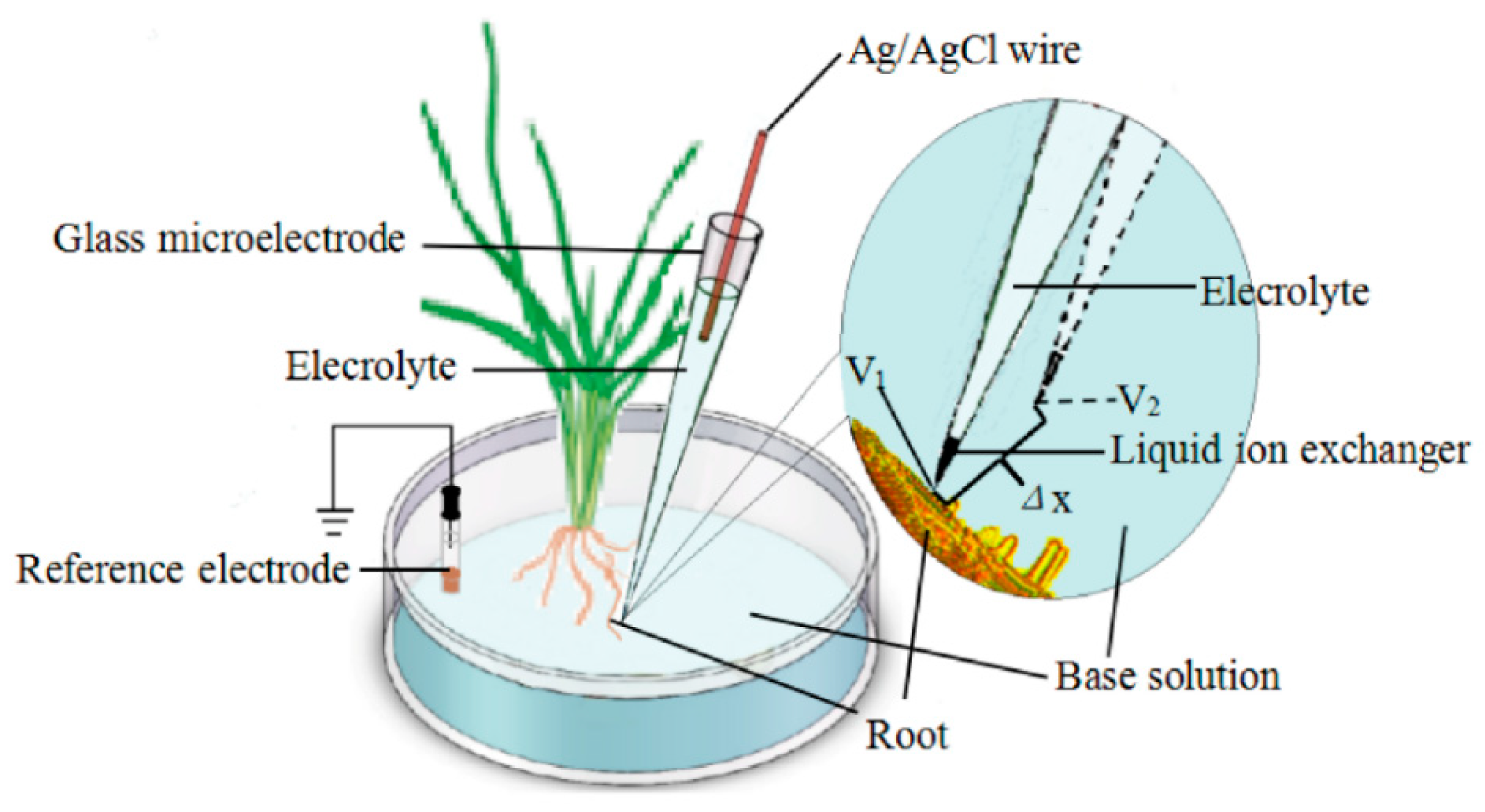
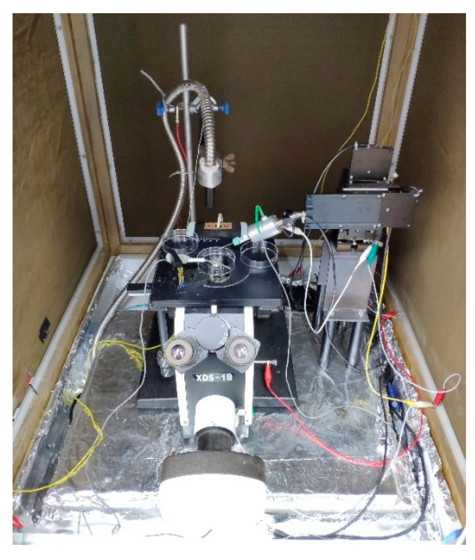
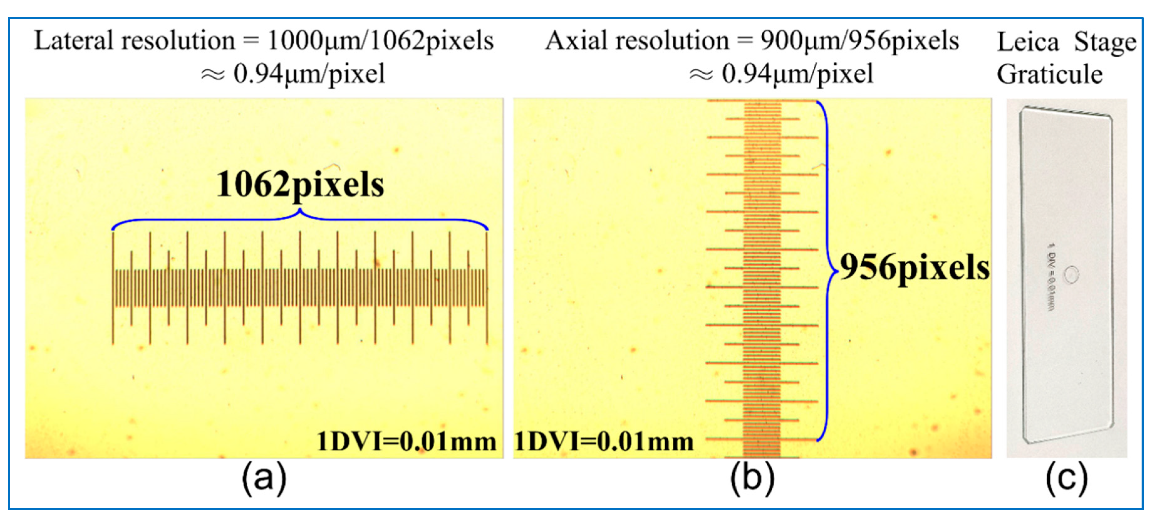
2.1. System Description

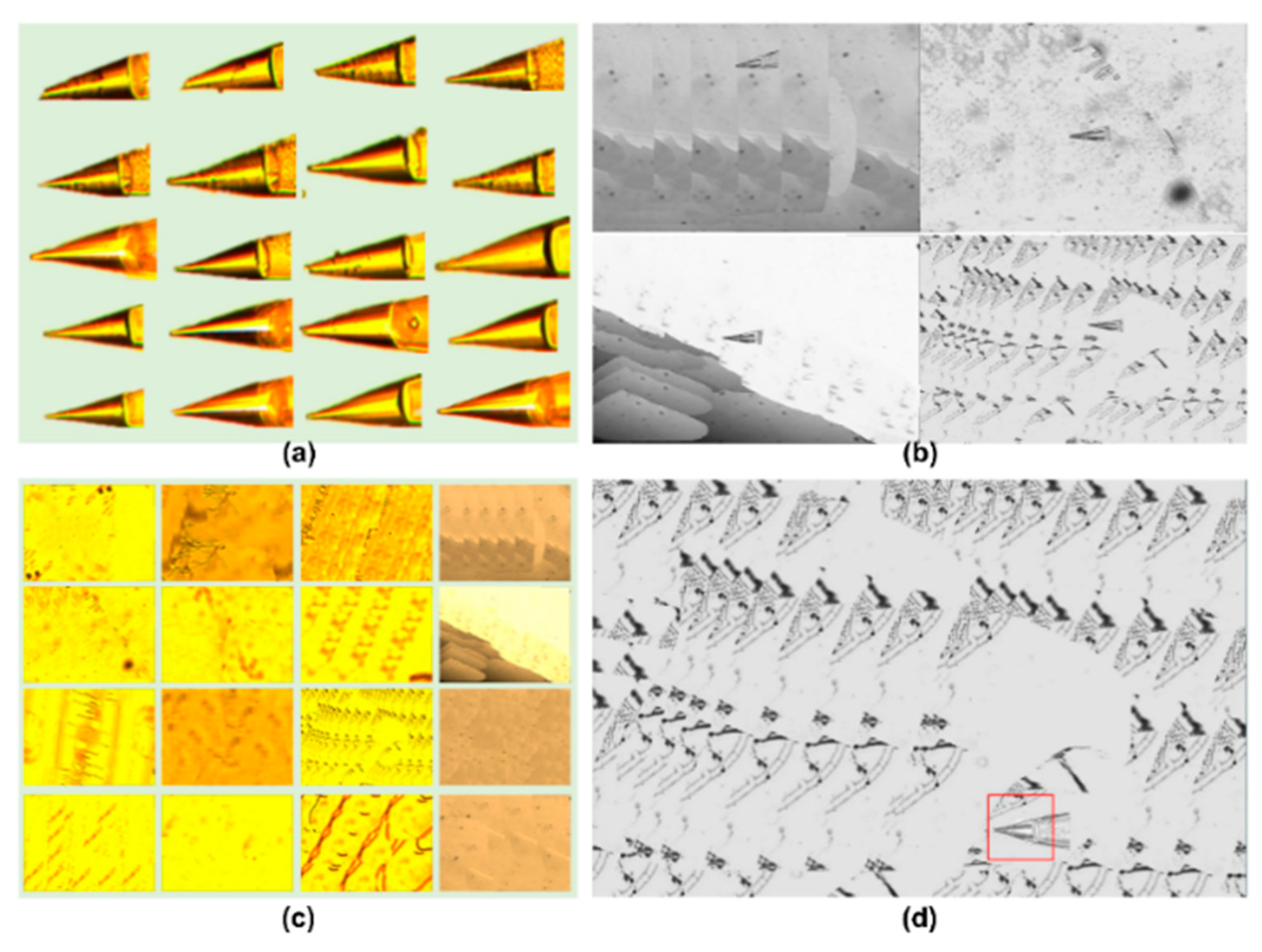
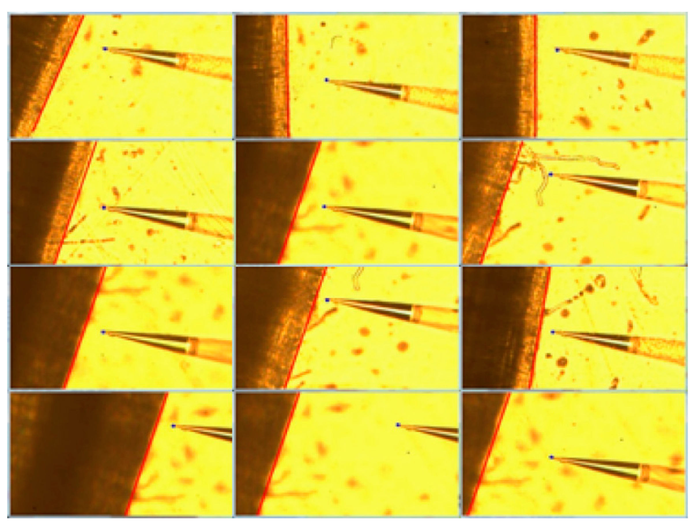
We acquired the images from our ion flux measurement system [13], as shown in Figure 3. The ion flux measurements consisted of an inverted microscope (XDS-1B, Chongqing MIC Technology Co, Ltd, Chongqing, China), a high-precision three-axis motorized manipulator (CFT-8301D, Jiangsu Rich Life Science Instrument Co., Ltd, Jiangsu, China), an ISME, a microelectrode holder, a multi-channel measurement software, and a charge coupled device (CCD) camera (TCC-1.4CHICE, Xintu Photonics, Fu Zhou, China). The ion flux and intracellular membrane potential were measured by a glass ion selective microelectrode. The two measured signals were amplified and transferred to the digital signals by the preamplifier and the 16-bit analogue-to-digital board (USB-4716, Advantech Co, Ltd, Taiwan, China) in the microelectrode holder. The digital signals were acquired by the multi-channel measurement software through a universal serial bus (USB) interface. The high-precision three-axis motorized manipulator was controlled by a personal computer (PC) through a USB interface. For more details, please refer to [13,19]. In the experiments, we obtained the images using a TCC-1.4CHICE (Xintu Photonics, Fu Zhou, China) CCD camera. The resolution of each image was 1360 × 1024 pixels, and the bit depth of the image was 24. The magnification of the microscope was 100X. The proposed vision-based measuring system was based on monocular vision. The CCD camera was mounted perpendicular to the working plane, and the position of the CCD camera and the internal and external parameters of the vision system were fixed. Because the purpose of the proposed system was for measuring the two-dimensional and relative distance of two micro-objects in the working plane, we did not need to get the world coordinates and camera coordinates of the micro-objects and calibrate the microscope imaging system—we only needed to get the axial and lateral resolution of the microscope imaging system. If researchers need the real location of the world coordinates and camera coordinates of the micro-objects, please refer to the [20,21]. We calculated the axial and lateral resolution of the image acquired by the CCD camera with the Leica Stage Graticule (1DIV (division value) = 0.01 mm) and TSView (Xintu Photonics, China) software. The calculation method was shown in Figure 4. Both the axial and lateral resolution of the microscope imaging system were 0.94 μm.

2.2. The Dataset

The original dataset was divided into a training set and a test set. Both the test set and the training set were composed of the real ISME images and the virtual samples generated by distorting, scaling, and adding noise to the background of the real ISME images. The virtual samples were generated with 5 real ISME images and 30 background images. The training set contained 6600 positive samples and 3000 negative samples. The test set contained 222 real ISME images obtained in different environments and 750 virtual samples.

In fact, it is a rather complex process to fabricate an ISME. It usually takes half a day or even one day to make a qualified ISME. Consequently, it is difficult to obtain enough samples in a short time. To solve this problem, we generated many virtual sample images by deforming and changing the scale of existing ISME images and combining these changed ISME images with different background images. In particular, this method allowed us to add various noises to the background images too. Though it led to a difficulty of ISME recognition of training data, it could help us to train the ISME recognition model with stronger robustness. Importantly, a large number of test samples can be generated to verify the ISME recognition model. To train a cascade classifier with high recognition rate and good robustness, the sample data must be large enough and abundant.

Figure 5 shows some real ISME images, background images with different exposure and noise conditions, the generated training samples, and the generated test samples.

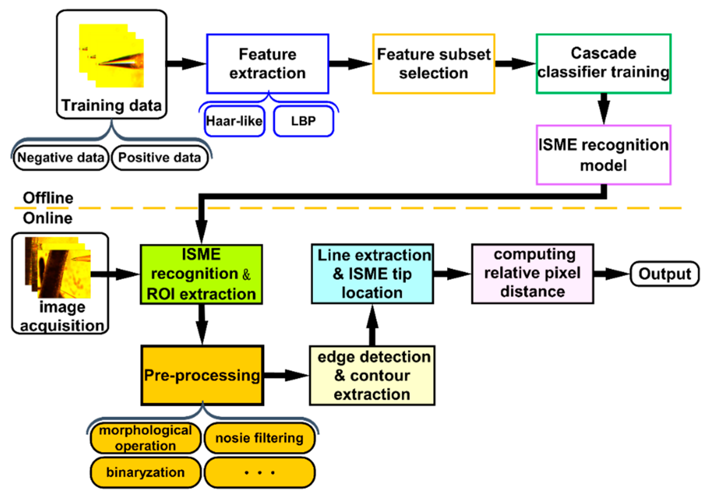
2.3. The Proposed Algorithm

The process of the proposed method for micro-object recognition and automatic relative distance calculation includes offline training and online detection (Figure 6). Offline training includes image acquisition, feature extraction, feature subset selection, and cascade classifier training. Online detection includes image acquisition, region of interest (ROI) acquisition, and image preprocessing (sharpening, filtering, morphological operations, etc.), edge detection, line extraction, ISME tip location, and relative distance calculation.

2.3.1. Image Preprocessing

The edge information of the images was the essential information for our purposes. The microscopic images collected by the CCD camera often contained lots of noise. For this reason, images had to be preprocessed. The image preprocessing of the test mainly included image filtering, sharpening, grayscale conversion, image binarization, and morphological operation.

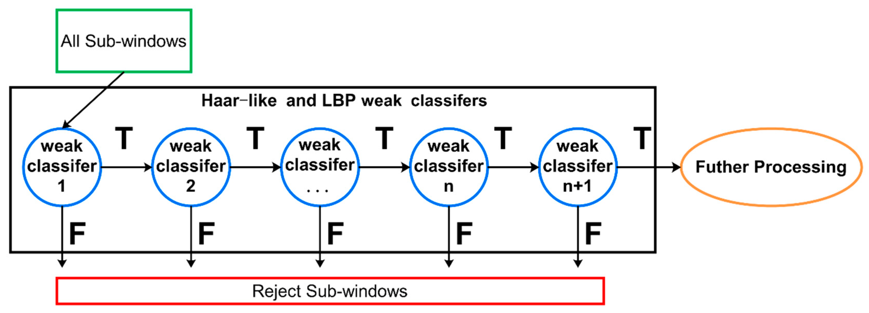
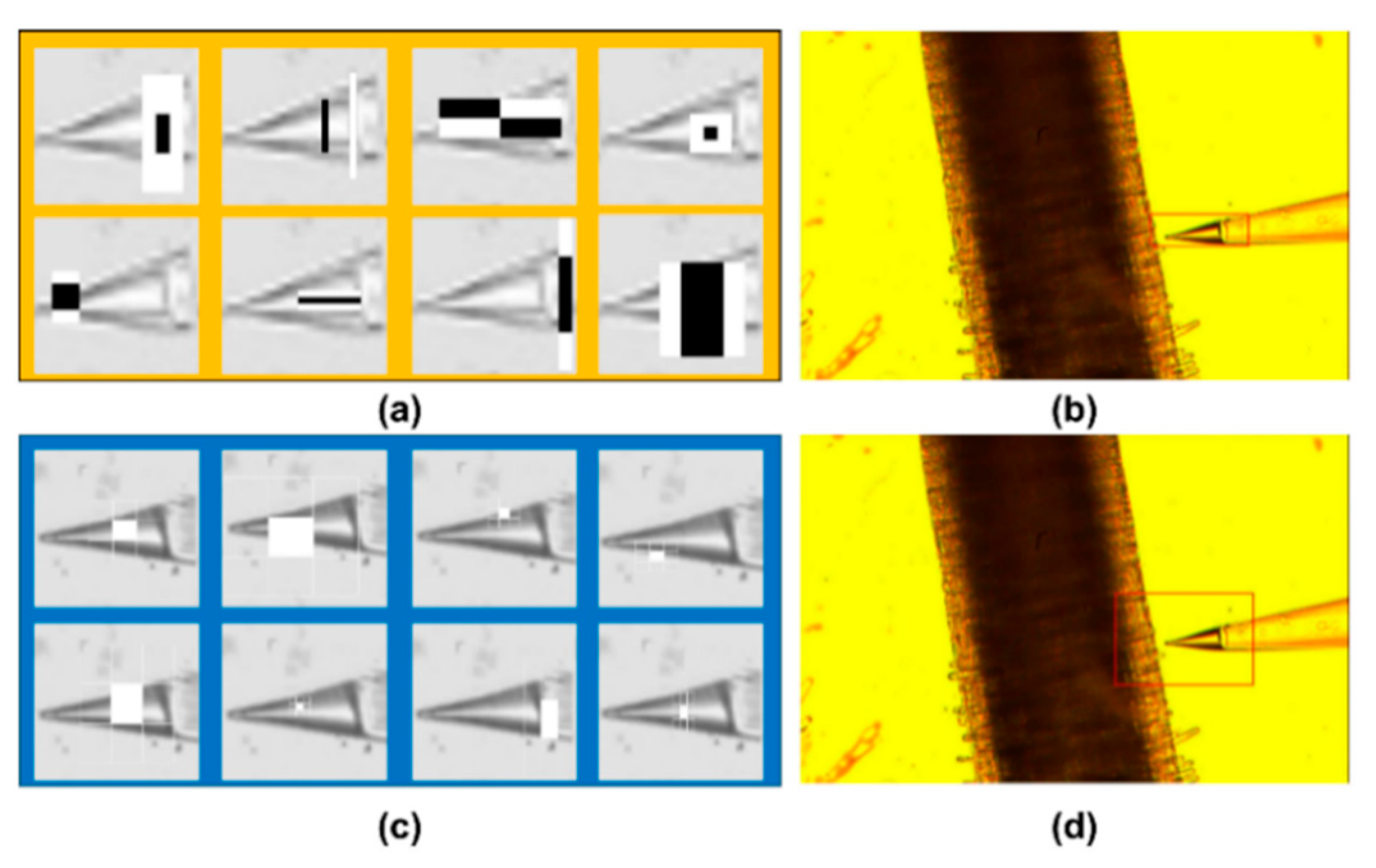
2.3.2. Training a Cascade Classifier for ISME

In this paper, the concept of the region of interest (ROI) was used to improve computation efficiency. Furthermore, we selected the area around the ISME that contained the root part as the ROI and then calculated the distance from the tip of the ISME to the root. In each experiment, there were some differences in every ISME’s shape. Additionally, some noise in the microscopic images, such as root hairs, microorganisms and impurities magnified by the microscope, could seriously affect the recognition of the ISME. For micro-object recognition in this work, there was still a challenge to determine the ROI. The traditional template matching method is sensitive to noise and does not have gray scale invariance and rotation invariance. Thus, in a complex environment, recognition accuracy is seriously affected. In addition, the traditional template matching method has a high computational cost, as it takes such a long time to recognize the ISME that cannot meet the real-time requirements well.

In a microscopic image, if the gray value of a mico-object is lower than that of the background environment, there is much more edge information. The improved Haar-like feature contains more edge information. Therefore, Haar-like features are suitable for ISME detection based on microscopic images. For detailed process, please refer to [22,23,24].

Besides rich local texture features, local binary pattern (LBP) features are also characterized by gray scale invariance and less computation [25]. Therefore, we can use LBP features and Haar-like features combined with an AdaBoost algorithm for rapid object recognition [22,26,27,28,29].

In the proposed method, AdaBoost is used to both select a small set of features and train the classifier. First, we extracted Haar-like features and LBP features of the ISME, and then we selected some distinct features for weak classifier training using the AdaBoost algorithm. For the detailed process, please refer to [30,31].

With ensemble learning, one can get a strong classifier by linearly combining some weak classifiers, which can greatly improve detection efficiency (Figure 7). Multi-feature fusion can effectively improve the detection rate of a cascade classifier. We can linearly combine both Haar-like classifiers and LBP classifiers to get a multi-feature cascade classifier. In this study, the Haar-like features and LBP features of an ISME were extracted and selected. Many weak classifiers based on Haar-like and LBP features were concatenated into strong cascade classifiers for ISME recognition. Then, we compared the strong cascade classifiers with the traditional template matching method.

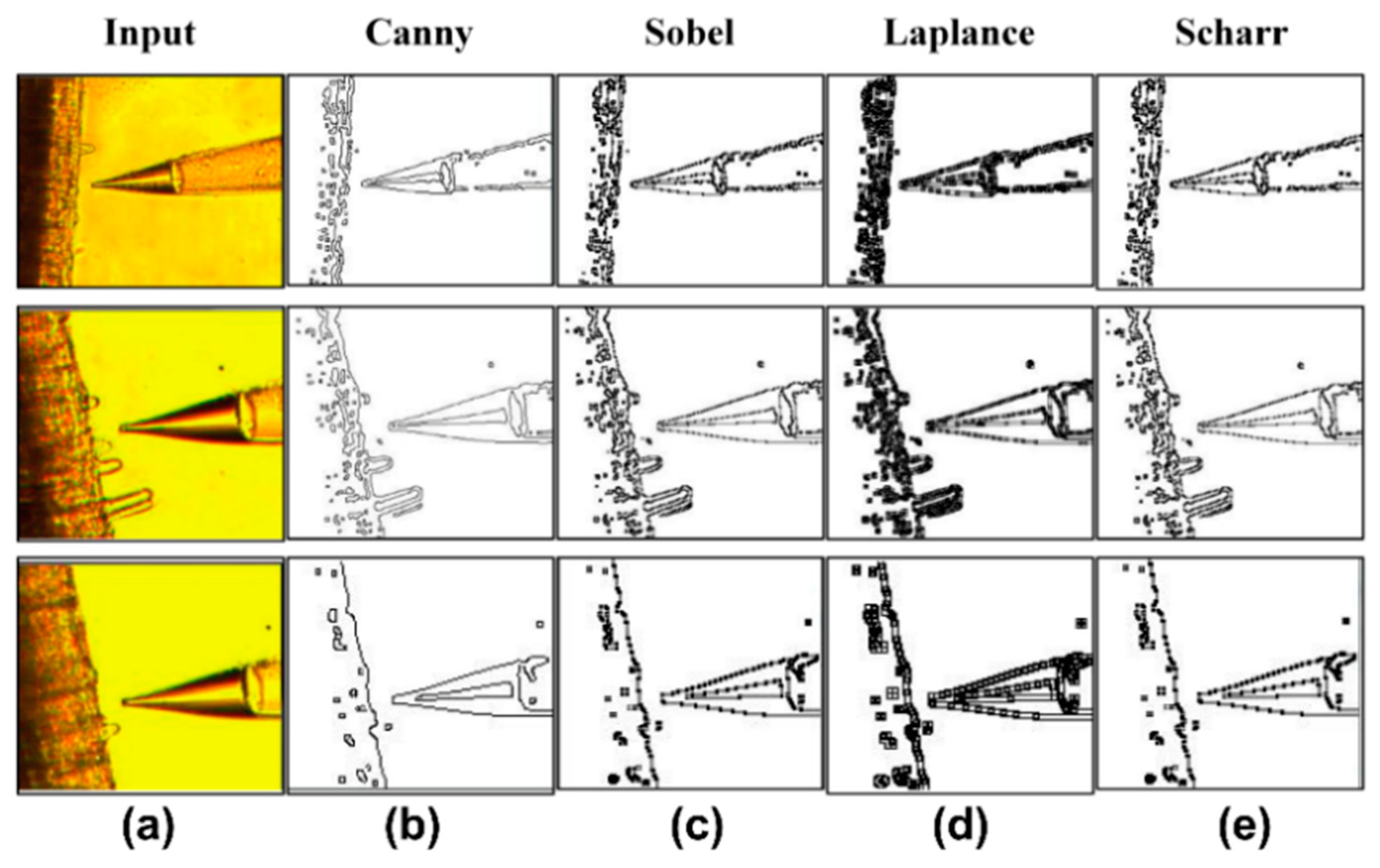
2.3.3. Edge Detection of the Target in the Microscopic Image

The useful information that we needed was the edge feature of the plant tissue and the ISME in microscopic field-of-view. After extracting the ROI and image preprocessing, edge detection was conducted. According to the differences of the filter, there are various image edge detection techniques, e.g., Canny edge detection, Sobel edge detection, Laplace edge detection, and Scharr edge detection. Sobel edge detection and Scharr edge detection are simpler than the others, but they are sensitive to noise and very error-prone. Laplace edge detection is able to find edges correctly, and it also has the ability to detect a wider neighborhood of pixels, but it is possible to make mistakes at the corners, flexure, and some areas where dimming and brightening are drastically changed. Canny edge detection is the most wildly used method, and it has a good ability for noise suppression [32,33], and it is mainly used to identify plant tissues and microelectrode edges.

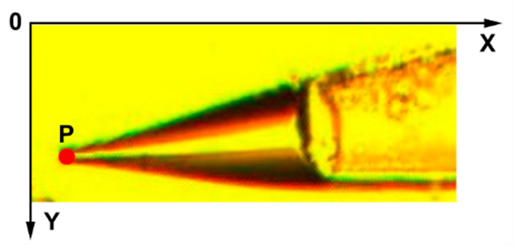
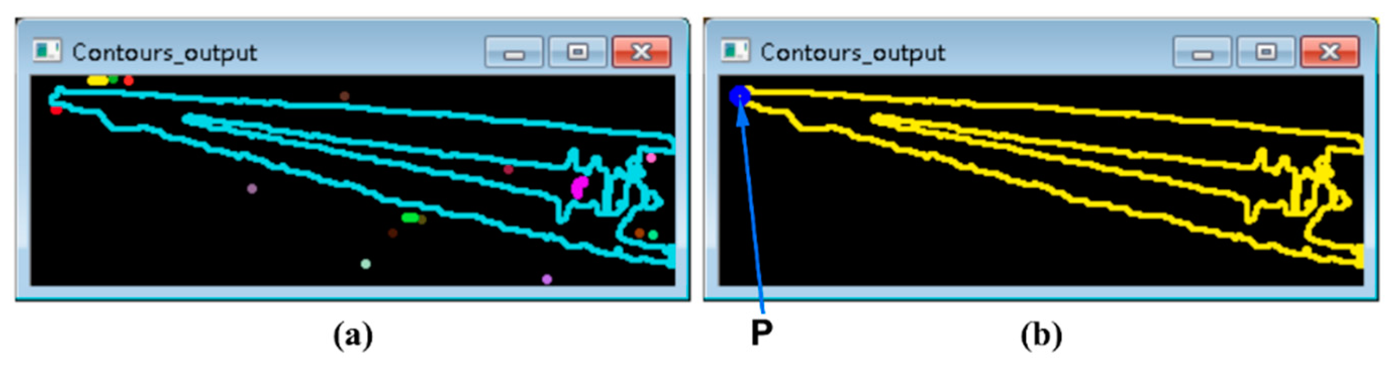
2.3.4. The Contour Extraction and the Localization of ISME Tip

In this work, the root and ISME were initially placed on the same x–y plane. Therefore, there was no need to consider spatial relations between them along the z-axis. For the root in the view of the microscope, the distance from the electrode tip to the root was the distance to the right edge of the root. The coordinate system of the image is shown in Figure 8. Therefore, to find the position of the ISME tip, we could firstly find the outermost contours of the ISME and traverse the pixels of the outermost contour. Where the point with the smallest value of x was the ISME tip represented by P. Due to the fact that the right edge of the root was an approximate straight line, Hough line detection could be performed on it. After the straight-line L was extracted, the distance d from the electrode tip P to the root edge (straight-line L) could be calculated. In order to detect the relative distance between the ISME tip and plant root, it was necessary to localize the ISME tip in microscopic field-of-view. Firstly, we extracted the outermost contours of the ISME.

Contour extraction was proposed by Suzuki and Abe [34], and it was used to extract the contours of ISME in our work. First, we found the outermost contour of the ISME. Then, we located the ISME tip. The ISME tip localization algorithm is described in Algorithm 1.

Algorithm 1: ISME Tip Localization

Input: edge_image Output: Tip Localization image is represented by tipLoc_image

BEGIN

1.Find Contours ()

2.For i = 0: contours.size//contours.size is the number of the contours

3.Get the length of all of the contours 4.END 5.Get the length of every contour 6.Con = the Longest contour 7.draw the Con on tipLoc_image

8.For j = 0: Con.size//Con.size is the size of Con 9.find the point named TIP with the minimum x// 10.draw a circle around the TIP

END

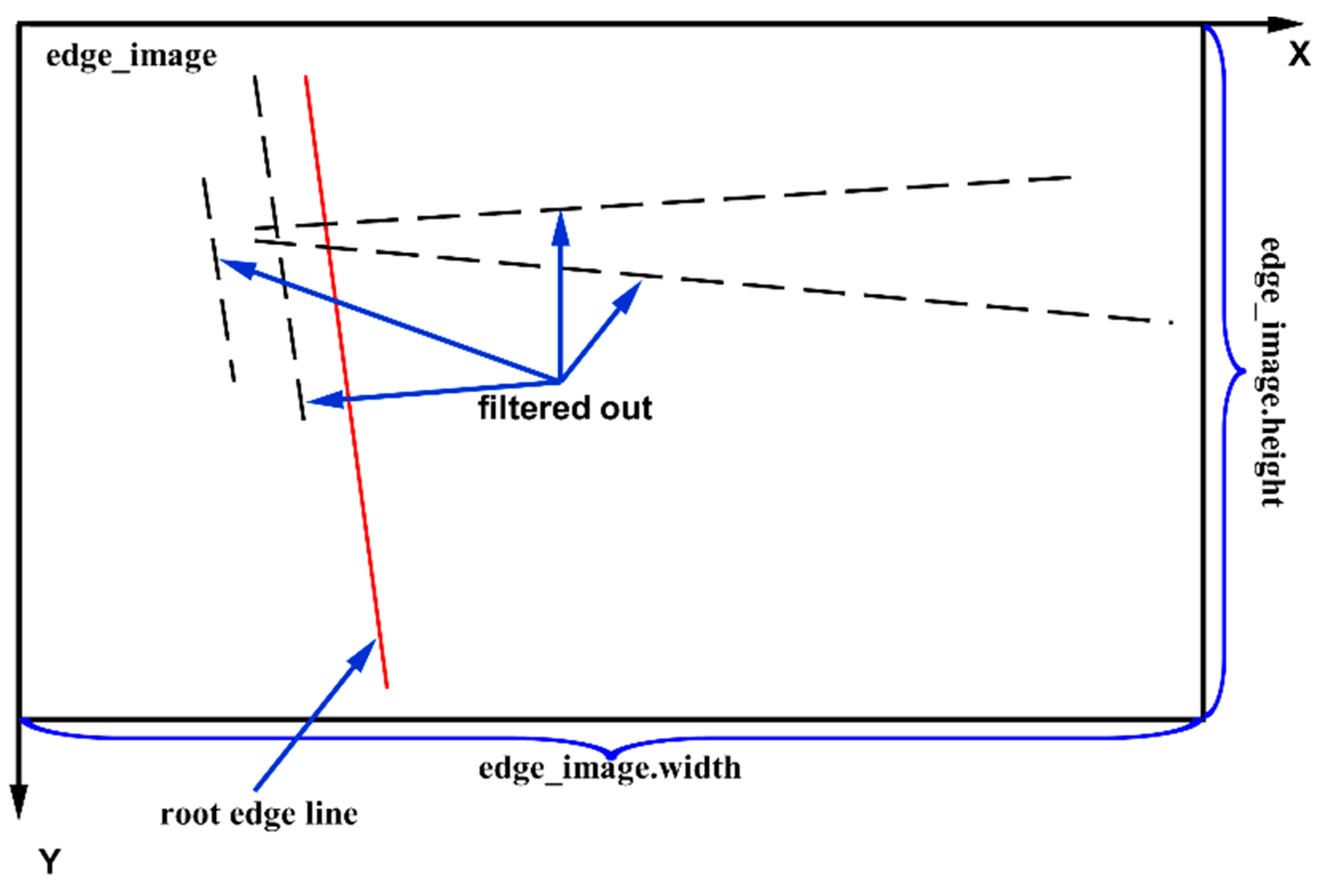
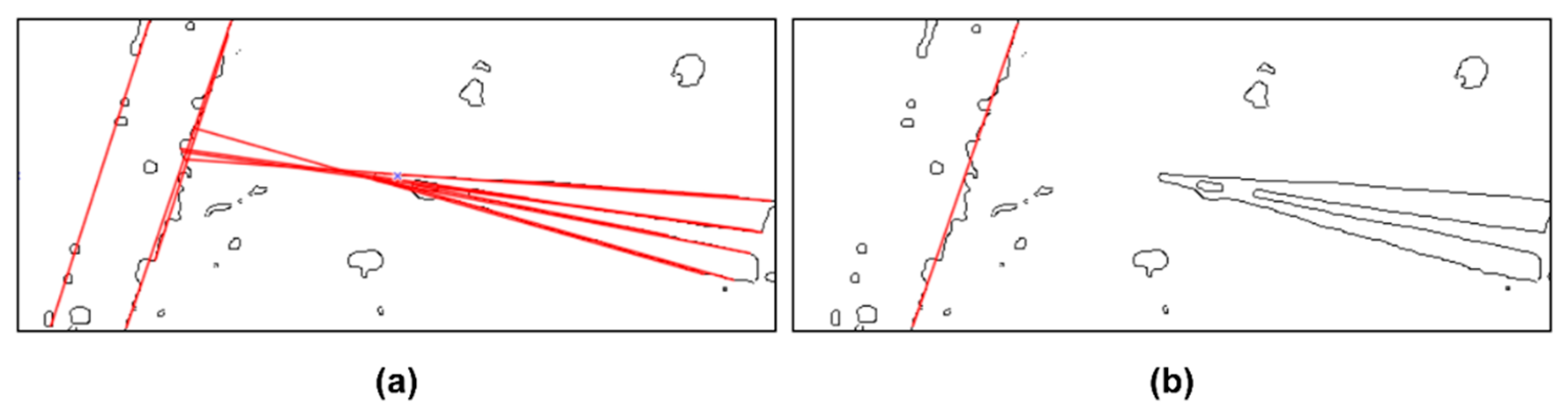
2.3.5. Edge Detection of Plant Root Using Hough Transformation

In order to detect the distance between the ISME and the plant root, it was necessary to detect the edge of the root in the microscopic field-of-view. Figure 2 shows that the local feature of the boundary of the main root could be approximated by a straight line. The widely used method for straight lines extraction in image processing is the Hough transformation [35].

We used the Hough transformation to detect the straight lines of the image, then screened and filtered the detected lines, and finally found the boundary of the main root. In order to allow the line to be filtered easily, we made the direction of the main root in the ROI vertical or approximately vertical (Figure 2). If the absolute value of the difference between the endpoints’ vertical coordinates of the extracted lines was bigger than three-quarters of the height of the ROI and the absolute value of the difference between the endpoints’ horizontal coordinates of the extracted lines was smaller than one third of the width of the ROI is, we retained the lines. Otherwise, we discarded the lines. This method helped us filter the lines, the directions of which were horizontal or approximately horizontal. The process of the root-edge-detection algorithm is described in Algorithm 2 and Figure 9.

Algorithm 2: Boundary Detection of Root

Input: edge_image Output: Tip Localization image is represented by tipLoc_image

BEGIN

1.plines = Hough Line detection of edge_image

2.For i = 0: plines.size//plines.size is the number of the lines 3.Point_A = A end point of plines segment Point_B = Another end point of plines segment

4.IF |Point_A.x–Point_B.x| < 1/3 edge_image.width & |Point_A.y – Point_B.y| > 3/4 edge_image.height 5.THEN retain the plines(i) Draw the plines(i) 6.ENDIF 7.END END

2.3.6. Distance Calculation

The pixel distance d from the tip P (x₀, y₀) to the straight-line L was calculated with Formula (2). We multiplied the d by the real-world distance corresponding to the pixel to get the real-world distance from P to L. Equation (2) is a general expression of a straight-line L, and Equation (3) is a distance formula from a point to a straight line. In Equation (4), D is the real-world distance from P to L, and α is the real-world distance corresponding to one pixel.

$$\mathrm{L}:\mathrm{A}x +\mathrm{B}y +\mathrm{C} =0$$

(1)

$$\mathrm{d}=\left|\frac{\mathrm{A}{x}_0+\mathrm{B}{y}_0+\mathrm{C}}{\sqrt{A^2+B^2}}\right|$$

(2)

$$\mathrm{D}=\mathrm{d}\times \mathsf{\alpha }$$

(3)

2.4. Experiments

In this study, all algorithms and experiments were performed with Visual Studio IDE (2015) with Intel(R) Core(TM) i5-4570 CPU. The training time of each classifier was recorded. To test the proposed algorithm, 800 test images were used as a test set on which the cascade classifiers and template matching algorithms were applied. The 800 test images consisted 50 real microscopic ISME images and 750 virtual samples. The total number of false positives (background was detected as the ISME) and true positives (the ISME was detected as ISME) were manually counted. When the intersection over union (IOU) value of the rectangle of the object label and the rectangle of the ISME detection is greater than 0.5, true positives count is increased by 1, otherwise false positives count is increased by 1. The true positive rate was used to evaluate the different methods of ISME detection. We also recorded the average time spent on ISME detection with each method. The true positive rate is defined as Equation (5) [22,23].

$$\mathrm{True}\mathrm{positive}\mathrm{rate}=\frac{Truepositives}{Turepositives +Falsepositives}\times 100\%$$

(4)

We labeled the ISME tips in 145 microscopic images and used the 145 labeled images as a test set to test the ISME tip location precision. We recorded the real-world distance from the ISME tip to the root in 25 images to test distance calculation precision of the proposed method. We calculated the root mean square error (RMS), mean error, and relative error [6,20]. The relative error of the tip location (${\mathrm{RE}}_T$) is defined as Equation (6), where ${\mathrm{A}}_{\mathrm{WP}}$ is the area of the working plane acquired by the CCD camera and $RM{S}_T$ is the root mean square error of the tip location of the test samples. The relative error of the relative distance of the micro-objects (${\mathrm{RE}}_D$) is defined as Equation (6), where $RM{S}_D$ is the root mean square error of the relative distance of the test samples and ${\mathrm{D}}_{\mathrm{M}}$ is the mean of the real-world distance of the test samples. The ${\mathrm{A}}_{\mathrm{WP}}$ is 1,230,536.7 ${\mathsf{\mu }\mathrm{m}}^2$ (1360 × 0.94 × 1024 × 0.94). The ${\mathrm{D}}_{\mathrm{M}}$ is 267.55$\mathsf{\mu }\mathrm{m}$.

$${\mathrm{RE}}_T=\frac{{\mathrm{RMS}}_{\mathrm{T}}{}^2}{{\mathrm{A}}_{\mathrm{WP}}}\times 100\%$$

(5)

$${\mathrm{RE}}_D=\frac{{\mathrm{RMS}}_{\mathrm{D}}}{{\mathrm{D}}_{\mathrm{M}}}\times 100\%$$

(6)

3. Results

3.1. Image Preprocessing

In image processing, the mainly need information is that of the edge of the image. The images collected by the camera often contain a lot of noise. Therefore, if the images are not preprocessed, which may affect the results of edge extraction and contour detection, even edge information and contours cannot be extracted.

The left three images in Figure 10 are the result of global binarization using the OTSU method [36], and the right three images are the result of local binarization using the adaptive threshold method [37,38]. The result shows that there was less noise in the result of global binarization using the OTSU method. Thus, the global binarization using adaptive threshold selection was better.

Though the image had been filtered and binarized, there were still some noise points and holes in it. We removed the remaining noise points and holes in the images by opening and closing the operation (Figure 11). The experiments showed that the noise was effectively suppressed and the features that we needed were highlighted.

3.2. ISME Cascade Classifier Training and ISME Detection

The tip of the ISME has recognizable characteristic from which the Haar-like and LBP features of the ISME tip can be extracted. With a gentle AdaBoost algorithm [39,40], we cascaded 30 different Haar-like feature-based weak classifiers and 30 different LBP feature-based weak classifiers to obtain two strong cascade classifiers for ISME tip detection. Some visualization images of the Haar-like and LBP features are shown in Figure 12. A typical case of ISME detection and ROI extraction results are shown in Figure 12. We used 800 test images to test the different detectors. According to the receiver operating characteristic (ROC) curve for the ISME detectors, cascade classifiers detectors were faster and more accurate than the template matching (TM) detectors, and the LBP cascade classifier had the best performance (Figure 13). Different ISME detectors had different levels of performance (

Table 1. Comparison of different ISME detectors.

Feature of Methods	Positive Samples Number	Negative Samples Number	Positive Samples Resolution (pixel)	Training Time (hours)	Average Test Time (s/frame)	Detection Rate
Haar-like	1118	1000	24 × 24	4.5	0.23	10.97%
LBP	1118	1000	24 × 24	1	0.30	4.31%
Haar-like	6600	3000	24 × 24	34	0.13	57.34%
LBP	6600	3000	24 × 24	4.78	0.21	47.22%
Haar-like	6600	3000	60 × 20	weeks	0.07	90.75%
LBP	6600	3000	60 × 20	26	0.13	92.73%
LBP	1118	1000	48 × 48	2.5	0.31	5.55%
LBP	6600	3000	48 × 48	28.5	1.14	50.82%
LBP	6600	3000	90 × 30	59.5	0.16	95.68%
LBP+Haar-like	6600	3000	90 × 30 (LBP)/60 × 20 (Haar-like)	--	0.23	99.14%
Templet-matching	--	--	--	--	0.33–0.44	17.50–39.95%

).

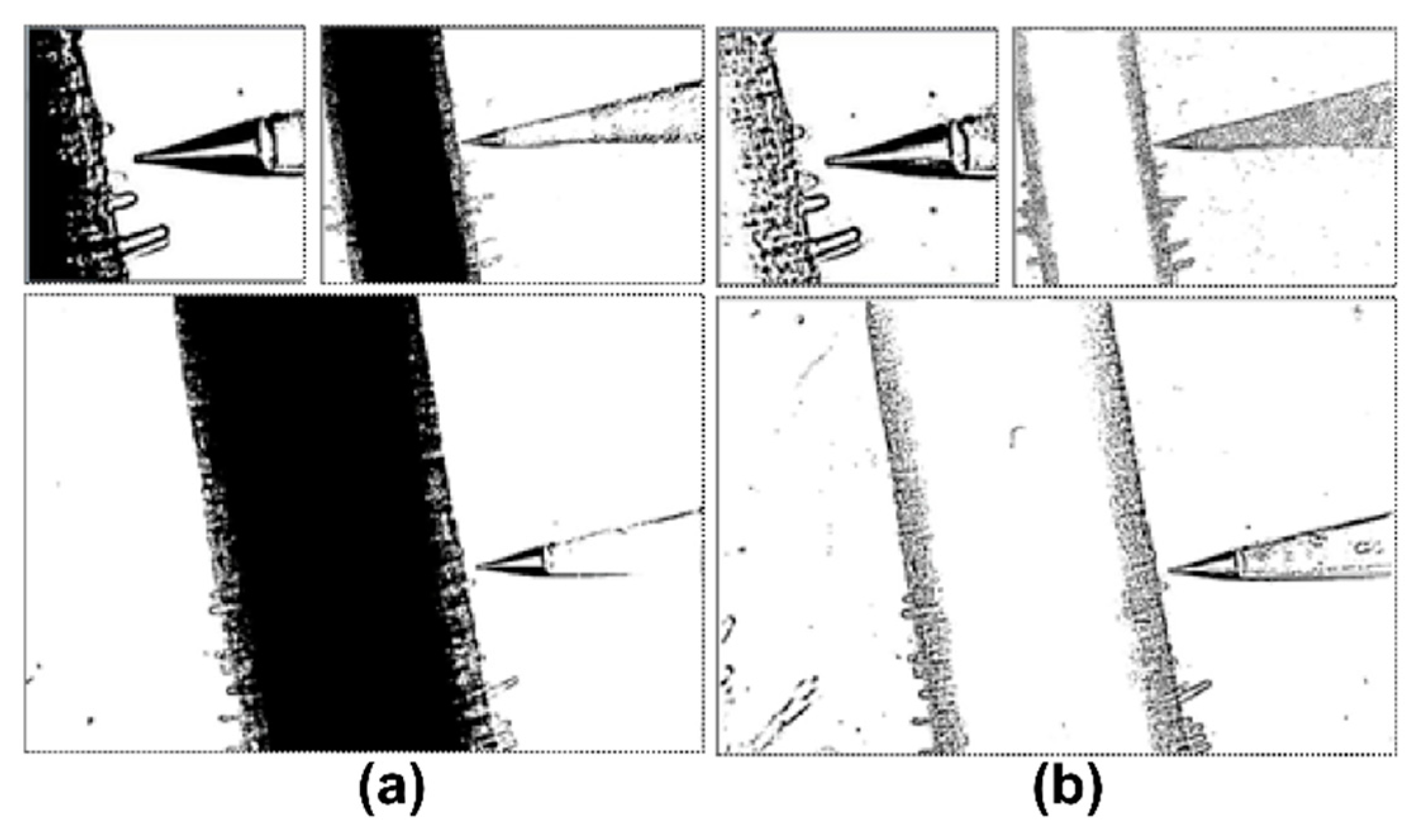
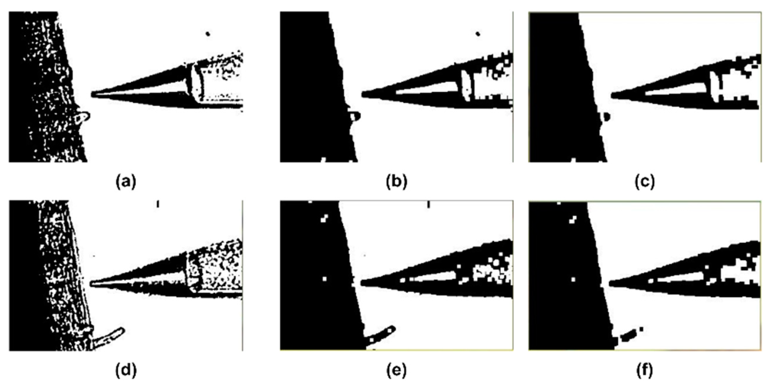
3.3. Edge Detection of Plant Tissues and Microelectrodes

We compared the detection performance of various edge detection techniques with the images of the ROI (Figure 14). Canny proposed three criteria for evaluating the performance of edge detection [32,33]:

(1)

The signal-to-noise ratio is higher.

(2)

The location of the edge points must be accurate; in other words, the detected edge points should be as close as possible to the center of the actual edge.

(3)

The detection must only have one response to a single edge, that is a single edge has only one unique response, and suppresses the response to false edge.

It can be seen from the figure that the effect of Canny edge detection was the best.

3.4. Contour Extraction and ISME Tip Localization

A contour extraction result is shown in Figure 15. Each color represents a separate contour, and the experiment showed that there were many contours in the image. The results of contours filtration and ISME tip location are shown in Figure 15b, where the blue point P is the position of the ISME.

To test the performance of the ISME-location algorithm, 145 images were used as a test set. Almost all the ISME tip could be correctly located (Figure 16 and Figure 17). The mean error was 2.86 μm, and the root mean square error was 2.89 μm. The ${\mathrm{RE}}_T$ was 0.000665%.

3.5. Edge Detection of Plant Root Using Hough Transformation

The result of the edge detection of main root is shown in Figure 18a. Obviously, there are many straight lines in the image. With the straight-lines screening, only the straight-line L extracted from the root edge was left (Figure 18b).

Figure 19 shows some results of the straight-line extraction and the ISME tip location.

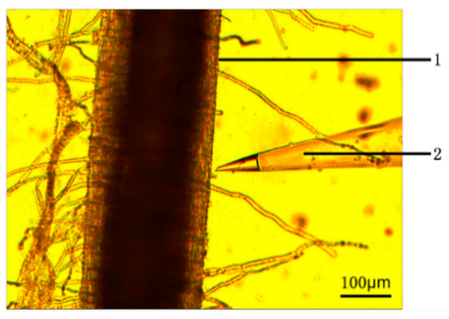
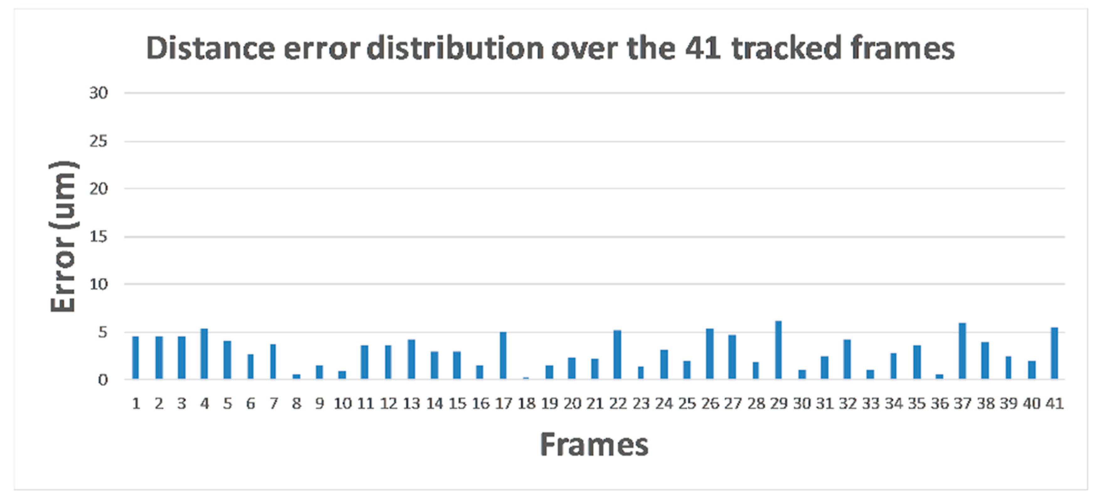
3.6. Computation of Relative Distance

In this case, the real-world distance corresponding to one pixel was 0.94 μm. We conducted an error analysis of the distance from the electrode tip to the root (n = 41) (Figure 20). The mean square error was 3.15 μm, and the root mean square error was 3.54 μm. The max distance error was 6.10 μm. The ${\mathrm{RE}}_D$ was 1.32%. The results indicate that the automatic detection of relative distance was more accurate than human eyes under these conditions.

4. Discussion

4.1. ISME Recognition

This research was intended to propose a method that can automatically and accurately calculate the relative distance between the two micro-objects in a microscopic image and facilitate automated micromanipulation research, e.g., ISME and detected objects.

In this work, ISME recognition using the proposed algorithm was a crucial step for subsequent operations. However, there were some differences in each ISME’s shape, and each ISME may have been randomly rotated to some angle in the experiment. The template matching-based algorithms were sensitive to noise without gray scale invariance and scale invariance. Accordingly, without continually changing the ISME templet in the ISME detection, the recognition rates could hardly meet the requirements (Figure 13). Besides that, the time cost of the template matching algorithm was higher than the best cascade classifier (Table 1).

The results suggest that the improved LBP features with the advantages of both gray scale invariance and scale invariance, as well as the Haar-like features with rich edge information, are suitable for object detection in complex situations (Table 1).

The performance of the proposed methods is dependent on image resolution and the amount of training data. Our results show that with the improvement of image resolution of training set, more effective features were detected, which improved the detection rate of classifiers but caused an increase of training time. When the training data set was small, the detection rate of Haar-like cascade classifier was slightly better than that of the LBP cascade classifier. With the increase of training data in the same resolution of training samples, the detection rate of the LBP cascade classifier was higher than that of the Haar-like cascade classifier. Additionally, the training time of the Haar-like cascade classifier was much longer than that of the LBP cascade classifier. When the resolution of the sample was relatively larger (e.g., 48 × 48) the training speed of the Haar-like cascade classifier became very slow—even the training of a weak classifier needed more than one day. Therefore, the LBP cascade classifier is a better choice when there is little difference in detection rate between the two kinds of classifiers. Between the ISME detection with Haar-like and LBP cascade classifiers, the Haar-like cascade classifiers had lower time costs. Therefore, Haar-like cascade classifiers are the better choice when real-time requirement is the primary choice. The cascade classifier with both Haar-like and LBP features had the best detection rate. This shows that the detection rate of an ISME cascade classifier can be improved by a multi-feature fusion method.

In the in-situ ion flux measurement process of a live tissue, the ISME was kept at 5–30 μm from the measured object to ensure accuracy and a growth speed of the root is 1–5 μm/min [13,19]. Thus, we needed monitor the root at least one time per minute. According to the processing time cost of each frame (Table 1), the frame rate could achieve 4.35–14 frames/s at a resolution of 1360 × 1024, which could perfectly meet the requirement.

In addition, the reasonable selection of training samples’ resolution could effectively reduce training time and improve detection rate. Because the width-to-height ratio of the ISME tip was about 3:1, when the width-to-width ratio of the training sample was 1:1, there was a large number of irrelevant pixels in the training sample. These irrelevant pixels increased the computation of feature extraction, thus increasing the training time. What is worse, some disturbing features were extracted from irrelevant pixels in the feature extraction process, which increased the difficulty of subsequent feature selection. The irrelevant pixels and disturbing features are shown in Figure 21. When the width-to-width ratio was 3:1, the training time was effectively reduced and the detection rate was greatly improved (Table 1).

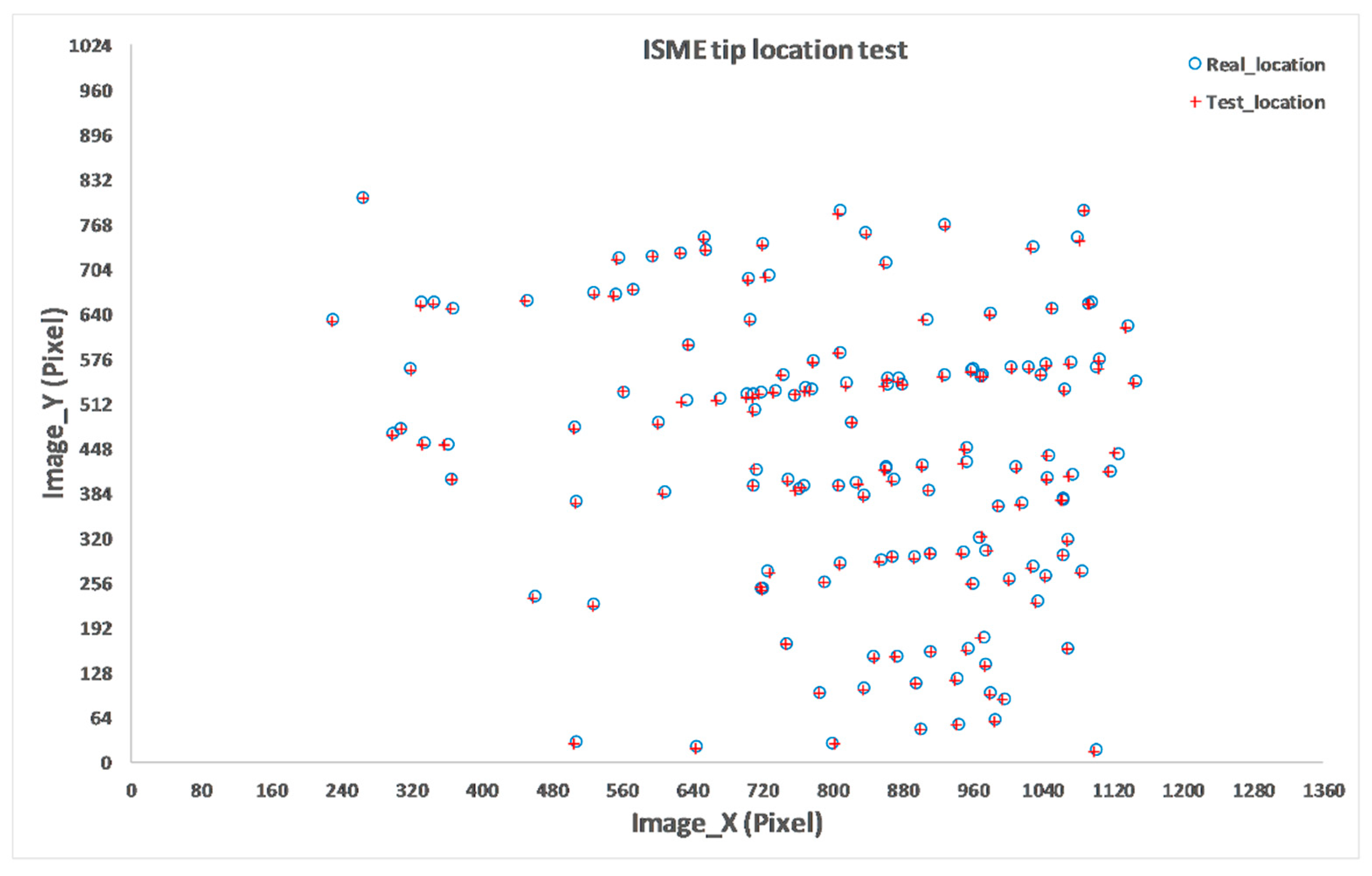
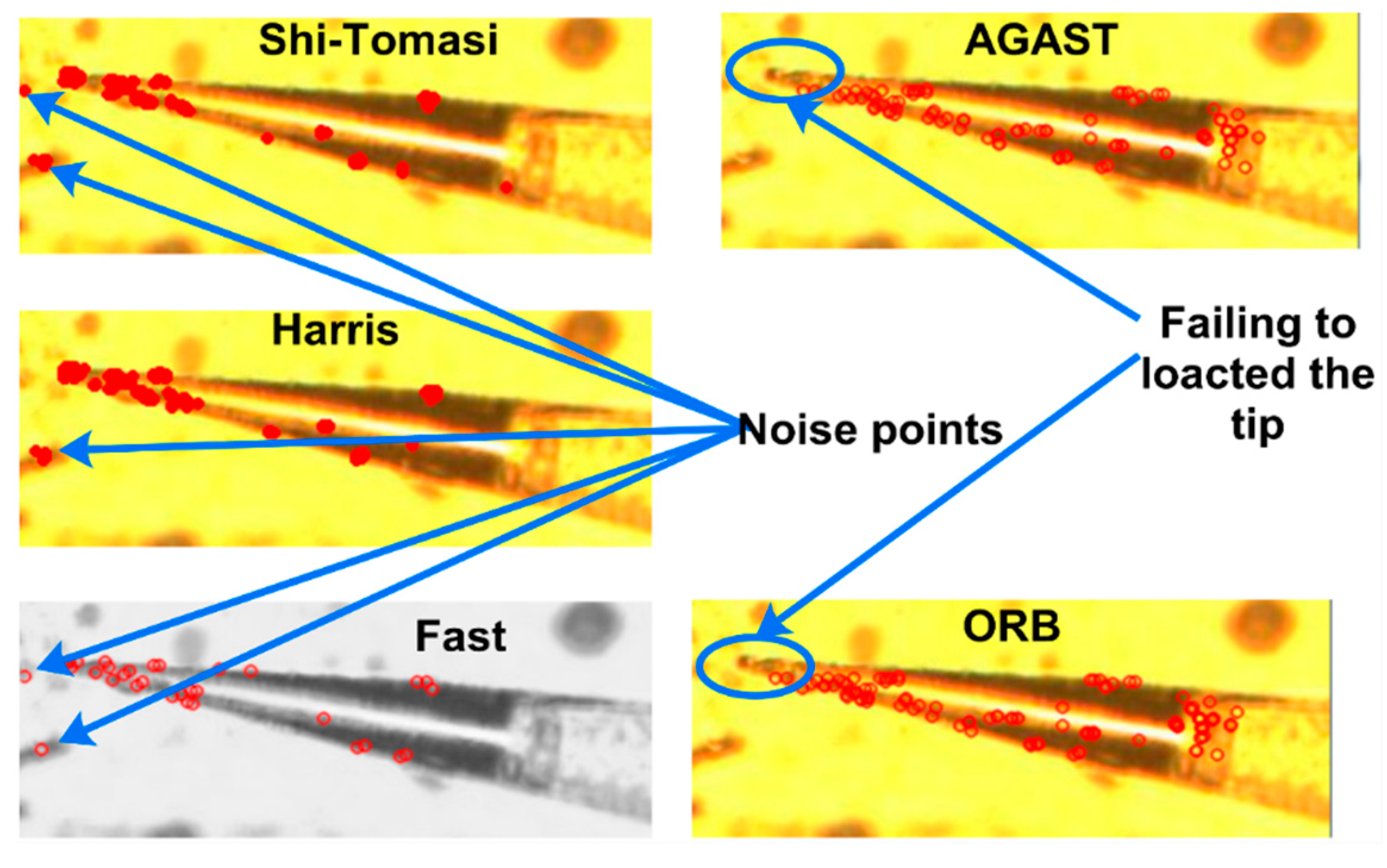
4.2. Location of the ISME Tip

The location of the electrode tip is the crucial step in the detection of the distance between the ISME tip and root, and its accuracy determines whether the distance can be correctly calculated. The proposed method could locate the ISME tip accurately with a mean error of 2.86 μm, a root mean square error of 2.89 μm, and an ${\mathrm{RE}}_T$ of 0.000665%. Normally, the distance between the ISME tip and the measured objects is 30 μm in the ion flux measurement. Therefore, this algorithm can well meet the accuracy requirement. Though almost all the ISME tips could be correctly located using the proposed algorithm (Figure 16), there were still a few exceptions, e.g., 55, 56, and 58 frames in Figure 22. It is the root hair that makes the ISME’s contour extraction inaccurate, which then allow for ISME tip locating failure (Figure 22). We could address this problem by increasing the limit of y direction and finding the point with the smallest y and x values. On the other hand, this reduces the flexibility of the ISME tip detection algorithm. This is a limitation of the algorithm. In the future, we will investigate the solution of this limitation.

We utilized tighter bounding boxes around the tip and then searching for corners inside the box. Therefore, the different corner detectors were used to locate the tip of ISME. Our experiments showed that this method was susceptible to noise points and was even not able to find the real tip of the ISME (Figure 23). The method used in our paper was a little more computationally intensive, but it had better robustness and accuracy.

4.3. Straight-Line Screening

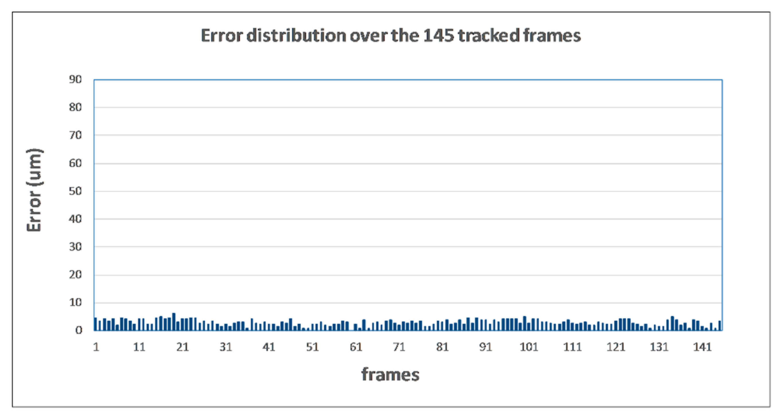
To calculate the relative distance between ISME and the root accurately, the root-edge straight line must be correctly and precisely extracted. Using the Hough transformation to detect straight lines in the ROI, the results show that there was more than one line, as shown in Figure 18a. In addition to the line extracted from the plant root, there were also straight lines extracted from the edge of the ISME. To pick out the lines that we needed, the parameters were also very important when we extracted the straight lines. If we set the appropriate value of the parameters, e.g., the maximum distance between two adjacent points and the minimum length of the lines that we extracted, we could filter the lines that were not long enough. Sometimes, there were several lines with the same or similar slopes around the root edge, as shown in Figure 18a. We could compute the intercept of these lines, and we were able to see that the line with the smallest intercept was the boundary of the roots. The coordinate system is shown in Figure 8.

4.4. Evaluation

Much research based on non-invasive micro-test technology (NMT) such as plant stress [41], plant heavy metal [42], growth and development [43], plant nutrition [44], plants and microbes interaction [45], and plant defense [46] are mainly conducted on a two-dimensional microscope imaging system. In all of these above, the measurement operations are performed by manually manipulating the electric motor under the microscope to further control the robot arm. The proposed method can facilitate the establishment of an automated micromanipulation system that can keep the distance between the selective microelectrode and the measured object safe, stable, and reliable and avoid their contact. The mean square error, the root mean square error, the max distance error, and the related error of the proposed automatic distance measurement algorithm is 3.15 μm, 3.54 μm. 6.10 μm, and 1.32%, respectively. Normally, the distance between the ISME tip and the objects to be measured is 30 μm in ion flux measurements. Thus, the proposed automatic distance-measurement algorithm can meet this requirement. The proposed method can not only ensure the accuracy and repeatability of measured data but also lighten the burden on researchers.

The purpose of the proposed system is to measure the two-dimensional and relative distance of two micro-objects in a working plane; thus, two advantages of this system are that we do not need to get the world coordinates and camera coordinates of the micro-objects and we do not need not to calibrate the microscope imaging system. The proposed method is simple to implement, but there are some disadvantages of the proposed method, such as this system not providing the real-world location of the world and camera coordinates of the micro-objects. This system is two-dimensional and does not provide three-dimensional information of the micro-objects. If researchers need the real-world location of the world coordinates, as well as the camera coordinates and the three-dimensional information of the micro-objects, the microscope imaging system should be additionally calibrated. Among the calibrations, there is both a strong anti-/interference ability and a good real-time performance of the calibration based on structured light [20]. Apolinar and Rodríguez [21] proposed a three-dimensional microscope vision system based on micro laser line scanning and adaptive genetic algorithms for retrieving metallic surface, and their system has a better performance compared with traditional systems, though its implementation is more complex. To sum up, the proposed method is simple and easy to implement, and it can be used in many applications based on micromanipulation and facilitate automated micromanipulation research. To address the limitation, researchers could add additional functions to this system based on their requirements.

5. Conclusions

Because of a wide range of applications, the study of automatic micromanipulation is very promising. A major advantage of the proposed method are that it adopts a more robust and faster microscopic object recognition algorithm to detect and locate microscopic objects and to calculate the distance between the two microscopic objects. Furthermore, this study can facilitate automated micromanipulation research. Another contribution of this work is that its provides a method for microscopic object recognition with a relatively small set of data by selecting suitable features to train the recognition model.

For a typical case, e.g., ion flux measurement by moving an ISME, we have proposed a more robust and faster microscopic object recognition and visual distance measurement algorithm with a better generalization ability. This algorithm can not only improve the efficiency of an ion flux measurement but also extend to other micromanipulation-related fields to aid automatic micromanipulation. In future research, we will optimize and accelerate the algorithm, and we will provide support for the automation of micromanipulation in broader applications in many research fields.

References

1. Shi, C.; Luu, D.K.; Yang, Q.; Liu, J.; Chen, J.; Ru, C.; Xie, S.; Luo, J.; Ge, J.; Sun, Y. Recent advances in nanorobotic manipulation inside scanning electron microscopes. Microsyst. Amp Nanoeng. 2016, 2, 16024. [Google Scholar] [CrossRef] [PubMed] [Green Version]
2. Wang, E.K.; Zhang, X.; Pan, L.; Cheng, C.; Dimitrakopoulou-Strauss, A.; Li, Y.; Zhe, N. Multi-Path Dilated Residual Network for Nuclei Segmentation and Detection. Cells 2019, 8, 499. [Google Scholar] [CrossRef] [PubMed]
3. Hung, J.; Carpenter, A. Applying faster R-CNN for object detection on malaria images. In Proceedings of the IEEE Conference on Computer Vision and Pattern Recognition Workshops, Honolulu, HI, USA, 21–26 July 2017; pp. 56–61. [Google Scholar]
4. Elsalamony, H.A. Detection of some anaemia types in human blood smears using neural networks. Meas. Sci. Technol. 2016, 27, 085401. [Google Scholar] [CrossRef]
5. Jayakody, H.; Liu, S.; Whitty, M.; Petrie, P. Microscope image based fully automated stomata detection and pore measurement method for grapevines. Plant Methods 2017, 13, 94. [Google Scholar] [CrossRef] [PubMed]
6. Yang, L.; Paranawithana, I.; Youcef-Toumi, K.; Tan, U. Automatic Vision-Guided Micromanipulation for Versatile Deployment and Portable Setup. IEEE Trans. Autom. Sci. Eng. 2018, 15, 1609–1620. [Google Scholar] [CrossRef]
7. Yang, L.; Youcef-Toumi, K.; Tan, U. Detect-Focus-Track-Servo (DFTS): A vision-based workflow algorithm for robotic image-guided micromanipulation. In Proceedings of the 2017 IEEE International Conference on Robotics and Automation (ICRA), Singapore, 29 May–3 June 2017; pp. 5403–5408. [Google Scholar]
8. Yang, L.; Paranawithana, I.; Youcef-Toumi, K.; Tan, U. Self-initialization and recovery for uninterrupted tracking in vision-guided micromanipulation. In Proceedings of the 2017 IEEE/RSJ International Conference on Intelligent Robots and Systems (IROS), Vancouver, BC, Canada, 24–28 September 2017; pp. 1127–1133. [Google Scholar]
9. Yang, L.; Youcef-Toumi, K.; Tan, U. Towards automatic robot-assisted microscopy: An uncalibrated approach for robotic vision-guided micromanipulation. In Proceedings of the 2016 IEEE/RSJ International Conference on Intelligent Robots and Systems (IROS), Daejeon, Korea, 9–14 October 2016; pp. 5527–5532. [Google Scholar]
10. Bilen, H.; Unel, M. Micromanipulation Using a Microassembly Workstation with Vision and Force Sensing. In Proceedings of the Advanced Intelligent Computing Theories and Applications. With Aspects of Theoretical and Methodological Issues, Berlin, Heidelberg, 15–18 September 2008; pp. 1164–1172. [Google Scholar]
11. Sun, Y.; Nelson, B.J. Biological Cell Injection Using an Autonomous MicroRobotic System. Int. J. Robot. Res. 2002, 21, 861–868. [Google Scholar] [CrossRef]
12. Saadat, M.; Hajiyavand, A.M.; Singh Bedi, A.-P. Oocyte Positional Recognition for Automatic Manipulation in ICSI. Micromachines 2018, 9, 429. [Google Scholar] [CrossRef]
13. Xue, L.; Zhao, D.-J.; Wang, Z.-Y.; Wang, X.-D.; Wang, C.; Huang, L.; Wang, Z.-Y. The calibration model in potassium ion flux non-invasive measurement of plants in vivo in situ. Inf. Process. Agric. 2016, 3, 76–82. [Google Scholar] [CrossRef] [Green Version]
14. Luxardi, G.; Reid, B.; Ferreira, F.; Maillard, P.; Zhao, M. Measurement of Extracellular Ion Fluxes Using the Ion-selective Self-referencing Microelectrode Technique. J. Vis. Exp. JoVE 2015, e52782. [Google Scholar] [CrossRef]
15. McLamore, E.S.; Porterfield, D.M. Non-invasive tools for measuring metabolism and biophysical analyte transport: Self-referencing physiological sensing. Chem. Soc. Rev. 2011, 40, 5308–5320. [Google Scholar] [CrossRef]
16. Lu, Z.; Chen, P.C.Y.; Nam, J.; Ge, R.; Lin, W. A micromanipulation system with dynamic force-feedback for automatic batch microinjection. J. Micromech. Microeng. 2007, 17, 314–321. [Google Scholar] [CrossRef]
17. Zhang, W.; Sobolevski, A.; Li, B.; Rao, Y.; Liu, X. An Automated Force-Controlled Robotic Micromanipulation System for Mechanotransduction Studies of Drosophila Larvae. IEEE Trans. Autom. Sci. Eng. 2016, 13, 789–797. [Google Scholar] [CrossRef]
18. Sun, F.; Pan, P.; He, J.; Yang, F.; Ru, C. Dynamic detection and depth location of pipette tip in microinjection. In Proceedings of the 2015 International Conference on Manipulation, Manufacturing and Measurement on the Nanoscale (3M-NANO), Changchun, China, 5–9 October 2015; pp. 90–93. [Google Scholar]
19. Wang, Z.; Li, J.; Zhou, Q.; Gao, X.; Fan, L.; Wang, Y.; Xue, L.; Wang, Z.; Huang, L. Multi-Channel System for Simultaneous In Situ Monitoring of Ion Flux and Membrane Potential in Plant Electrophysiology. IEEE Access 2019, 7, 4688–4697. [Google Scholar] [CrossRef]
20. Apolinar Muñoz Rodríguez, J. Microscope self-calibration based on micro laser line imaging and soft computing algorithms. Opt. Lasers Eng. 2018, 105, 75–85. [Google Scholar] [CrossRef]
21. Apolinar, J.; Rodríguez, M. Three-dimensional microscope vision system based on micro laser line scanning and adaptive genetic algorithms. Opt. Commun. 2017, 385, 1–8. [Google Scholar] [CrossRef]
22. Viola, P.; Jones, M. Rapid object detection using a boosted cascade of simple features. In Proceedings of the 2001 IEEE Computer Society Conference on Computer Vision and Pattern Recognition. CVPR 2001, Kauai, HI, USA, 8–14 December 2001; p. 3. [Google Scholar]
23. Zhao, Y.; Gong, L.; Zhou, B.; Huang, Y.; Liu, C. Detecting tomatoes in greenhouse scenes by combining AdaBoost classifier and colour analysis. Biosyst. Eng. 2016, 148, 127–137. [Google Scholar] [CrossRef]
24. Yu, Y.; Ai, H.; He, X.; Yu, S.; Zhong, X.; Lu, M. Ship Detection in Optical Satellite Images Using Haar-like Features and Periphery-Cropped Neural Networks. IEEE Access 2018, 6, 71122–71131. [Google Scholar] [CrossRef]
25. Ojala, T.; Pietikainen, M.; Maenpaa, T. Multiresolution gray-scale and rotation invariant texture classification with local binary patterns. IEEE Trans. Pattern Anal. Mach. Intell. 2002, 24, 971–987. [Google Scholar] [CrossRef]
26. Wen, X.; Shao, L.; Xue, Y.; Fang, W. A rapid learning algorithm for vehicle classification. Inf. Sci. 2015, 295, 395–406. [Google Scholar] [CrossRef]
27. Wen, X.; Shao, L.; Fang, W.; Xue, Y. Efficient Feature Selection and Classification for Vehicle Detection. IEEE Trans. Circuits Syst. Video Technol. 2015, 25, 508–517. [Google Scholar] [CrossRef]
28. Cheng, G.; Han, J. A survey on object detection in optical remote sensing images. ISPRS J. Photogramm. Remote Sens. 2016, 117, 11–28. [Google Scholar] [CrossRef] [Green Version]
29. Ahonen, T.; Hadid, A.; Pietikainen, M. Face description with local binary patterns: Application to face recognition. IEEE Trans. Pattern Anal. Mach. Intell. 2006, 28, 2037–2041. [Google Scholar] [CrossRef] [PubMed]
30. Freund, Y.; Schapire, R.E. A Decision-Theoretic Generalization of On-Line Learning and an Application to Boosting. J. Comput. Syst. Sci. 1997, 55, 119–139. [Google Scholar] [CrossRef] [Green Version]
31. Viola, P.; Jones, M.J. Robust Real-Time Face Detection. Int. J. Comput. Vis. 2004, 57, 137–154. [Google Scholar] [CrossRef]
32. Maini, R.; Aggarwal, H. Study and comparison of various image edge detection techniques. Int. J. Image Process. (IJIP) 2009, 3, 1–11. [Google Scholar]
33. Canny, J. A computational approach to edge detection. IEEE Trans. Pattern Anal. Mach. Intell. 1986, 6, 679–698. [Google Scholar] [CrossRef]
34. Suzuki, S.; Abe, K. Topological structural analysis of digitized binary images by border following. Comput. Vis. Graph. Image Process. 1985, 30, 32–46. [Google Scholar] [CrossRef]
35. Duda, R.O.; Hart, P.E. Use of the Hough transformation to detect lines and curves in pictures. Commun. ACM 1972, 15, 11–15. [Google Scholar] [CrossRef]
36. Otsu, N. A threshold selection method from gray-level histograms. IEEE Trans. Syst. Man Cybern. 1979, 9, 62–66. [Google Scholar] [CrossRef]
37. Bradley, D.; Roth, G. Adaptive thresholding using the integral image. J. Graph. Tools 2007, 12, 13–21. [Google Scholar] [CrossRef]
38. Wellner, P.D. Adaptive thresholding for the DigitalDesk. Xerox EPC1993-110 1993, 110, 1–19. [Google Scholar]
39. Schapire, R.E.; Singer, Y. Improved Boosting Algorithms Using Confidence-rated Predictions. Mach. Learn. 1999, 37, 297–336. [Google Scholar] [CrossRef] [Green Version]
40. Kuang, H.; Chong, Y.; Li, Q.; Zheng, C. MutualCascade method for pedestrian detection. Neurocomputing 2014, 137, 127–135. [Google Scholar] [CrossRef]
41. Ma, Y.; Dai, X.; Xu, Y.; Luo, W.; Zheng, X.; Zeng, D.; Pan, Y.; Lin, X.; Liu, H.; Zhang, D.; et al. COLD1 Confers Chilling Tolerance in Rice. Cell 2015, 160, 1209–1221. [Google Scholar] [CrossRef] [Green Version]
42. Ma, J.; Zhang, X.; Zhang, W.; Wang, L. Multifunctionality of Silicified Nanoshells at Cell Interfaces of Oryza sativa. ACS Sustain. Chem. Eng. 2016, 4, 6792–6799. [Google Scholar] [CrossRef]
43. Bai, L.; Ma, X.; Zhang, G.; Song, S.; Zhou, Y.; Gao, L.; Miao, Y.; Song, C.-P. A Receptor-Like Kinase Mediates Ammonium Homeostasis and Is Important for the Polar Growth of Root Hairs in Arabidopsis. Plant Cell 2014, 26, 1497–1511. [Google Scholar] [CrossRef]
44. Han, Y.-L.; Song, H.-X.; Liao, Q.; Yu, Y.; Jian, S.-F.; Lepo, J.E.; Liu, Q.; Rong, X.-M.; Tian, C.; Zeng, J.; et al. Nitrogen Use Efficiency Is Mediated by Vacuolar Nitrate Sequestration Capacity in Roots of Brassica napus. Plant Physiol. 2016, 170, 1684–1698. [Google Scholar] [CrossRef]
45. Ma, Y.; He, J.; Ma, C.; Luo, J.; Li, H.; Liu, T.; Polle, A.; Peng, C.; Luo, Z.-B. Ectomycorrhizas with Paxillus involutus enhance cadmium uptake and tolerance in Populus × canescens. Plant Cell Environ. 2014, 37, 627–642. [Google Scholar] [CrossRef]
46. Chen, H.; Zhang, Y.; He, C.; Wang, Q. Ca2+ Signal Transduction Related to Neutral Lipid Synthesis in an Oil-Producing Green Alga Chlorella sp. C2. Plant Cell Physiol. 2014, 55, 634–644. [Google Scholar] [CrossRef]
Figure 1. The principle of ion flux measurement. Notes: V1 and V2 are the measured voltages for different gradients at two positions in distance Δx using the ion-selective microelectrode (ISME), mV, and Δx is the distance between two positions where the ISME vibrated (μm). E   =   k   ±   slgC , where E is the measured voltage between the microelectrode and the reference electrode (mV), C is the ion concentration (mol/L), s is Nernstian slope (mV/dec); k is Nernstian intercept (mV).
Algorithms 12 00238 g001
Figure 2. Typical microscopy image of biological experiment. 1. Wheat root; 2. ISME.
Algorithms 12 00238 g002
Figure 3. The ion flux measurements system.
Algorithms 12 00238 g003
Figure 4. (a): The calculation of the lateral resolution; (b): the calculation of the axial resolution; (c): Leica Stage Graticule.
Algorithms 12 00238 g004
Figure 5. (a): The real ISME images; (b): the background images under different light and noise conditions (c): virtual samples; (d): the generated test samples.
Algorithms 12 00238 g005
Figure 6. The flowchart of machine learning-based ISME recognition and relative distance computation.
Algorithms 12 00238 g006
Figure 7. Schematic depiction of the detection cascade.
Algorithms 12 00238 g007
Figure 8. The coordinate system of the image.
Algorithms 12 00238 g008
Figure 9. The process of screening straight lines.
Algorithms 12 00238 g009
Figure 10. (a): The left three images are the results of global adaptive threshold selection binarization. (b): The right three images are the results of local adaptive threshold binarization.
Algorithms 12 00238 g010
Figure 11. (a,b) are two binarized images, (c,d) are binary images after the open operation, and (e,f) are binary images after the close operation.
Algorithms 12 00238 g011
Figure 12. Extracting the region of interest (ROI). Note: (a) is the visualization of some Haar-like features of ISME tip; (b) is the recognition result of the ISME tip; (c) is the visualization of some local binary pattern (LBP) features of the ISME tip; and (d) is the result of ROI extraction.
Algorithms 12 00238 g012
Figure 13. ROC curve for ISME detectors with stepsize = 1.0.
Algorithms 12 00238 g013
Figure 14. The results of edge detection of various image edge detection techniques. (a) Input images; (b) Canny edge detection results; (c) Sobel edge detection results; (d) Laplace edge detection results; and (e) Scharr edge detection results.
Algorithms 12 00238 g014
Figure 15. Contour extraction and ISME tip localization. Note: (a) is the output image of contour extraction, and (b) is the output image of the outermost contour selection and the ISME tip location. P is the ISME tip.
Algorithms 12 00238 g015
Figure 16. The ISME tip location test result of 145 images.
Algorithms 12 00238 g016
Figure 17. Error distribution over the 145 tracked frames.
Algorithms 12 00238 g017
Figure 18. (a): Line extraction. (b): Line screening.
Algorithms 12 00238 g018
Figure 19. Tip of ISME and root identification.
Algorithms 12 00238 g019
Figure 20. Distance error distribution over the 41 tracked frames.
Algorithms 12 00238 g020
Figure 21. Irrelevant pixels and disturbing features.
Algorithms 12 00238 g021
Figure 22. Failure ISME tip locations.
Algorithms 12 00238 g022
Figure 23. Corner detection using different methods.
Algorithms 12 00238 g023