Stability Analysis of Jacobian-Free Newton’s Iterative Method

Abstract

It is well known that scalar iterative methods with derivatives are highly more stable than their derivative-free partners, understanding the term stability as a measure of the wideness of the set of converging initial estimations. In multivariate case, multidimensional dynamical analysis allows us to afford this task and it is made on different Jacobian-free variants of Newton’s method, whose estimations of the Jacobian matrix have increasing order. The respective basins of attraction and the number of fixed and critical points give us valuable information in this sense.

1. Introduction

Let $F\left(x\right)=0$, $F:D\subseteq {\mathbb{R}}^n⟶{\mathbb{R}}^n$, be a system of nonlinear equations. Usually, this kind of problems can not be solved analytically and the approach to a solution is made by means of iterative techniques. The best known iterative algorithm is Newton’s method, with second order of convergence and iterative expression

$$\begin{array}{c}\hfill x^{(k+1)}=x^{\left(k\right)}-{\left[F^{\prime }\left(x^{\left(k\right)}\right)\right]}^{-1}F\left(x^{\left(k\right)}\right),k=0,1,\dots \end{array}$$

(1)

from an estimation $x^{\left(0\right)}\in D$. This iterative scheme needs the evaluation of the nonlinear function and its associate Jacobian matrix at each iteration. However, sometimes, the size of the system or the specific properties of the problem do not allow to evaluate the Jacobian matrix $F^{\prime }\left(x\right)$, or even its calculation at each iteration (for example, if F is an error function); in these cases, some approximations of the Jacobian matrix can be used. The most usual one is a divided difference matrix, that is, a linear operator $[x^{\left(k\right)},y^{\left(k\right)};F]$ satisfying condition (see [1,2])

$$\begin{array}{c}\hfill [x,y;F](x-y)=F\left(x\right)-F\left(y\right).\end{array}$$

(2)

In this case, when $F^{\prime }\left(x^{\left(k\right)}\right)$ in Newton’s method is replaced by $[x^{\left(k\right)},y^{\left(k\right)};F]$, where $y=x^{\left(k\right)}+F\left(x^{\left(k\right)}\right)$, we obtain the so-called Steffensen’s method [1], also with order of convergence two. To compute in practice the elements of the divided difference operator, the following first-order divided difference operator

$$\begin{array}{c}\hfill {[x^{\left(k\right)},y^{\left(k\right)};F]}_{i,j}^1=\frac{F_i(y_1,y_2,\dots ,y_{j-1},y_j,x_{j+1},\dots ,x_n)-F_i(y_1,y_2,\dots ,y_{j-1},x_j,x_{j+1},\dots ,x_n)}{y_j-x_j},\end{array}$$

(3)

or the symmetric second-order one,

$$\begin{array}{c}{[x^{\left(k\right)},y^{\left(k\right)};F]}_{i,j}^2=(F_i(y_1,y_2,\dots ,y_{j-1},y_j,x_{j+1},\dots ,x_n)-F_i(y_1,y_2,\dots ,y_{j-1},x_j,x_{j+1},\dots ,x_n)\hfill \\ +F_i(x_1,x_2,\dots ,x_{j-1},x_j,y_{j+1},\dots ,y_n)-F_i(x_1,x_2,\dots ,x_{j-1},y_j,y_{j+1},\dots ,y_n))/\left(2(y_j-x_j)\right),\hfill \end{array}$$

(4)

are proposed in [3].

Let us remark that operator (4) is symmetric and it can be used to evaluate the divided difference even when the problem is nonsymmetric. However, the number of evaluations of the scalar functions in the computation of (4) is higher than those in (3). Moreover, when divided difference (3) is used as an approximation for the Jacobian matrices appearing in any iterative method, then usually the iterative procedure does not preserve its order of convergence.

The authors in [4] proposed to replace $y=x+F\left(x\right)$ in (2) by $y=x+\Gamma \left(x\right)$, being $\Gamma \left(x\right)={(f_1{\left(x\right)}^m,f_2{\left(x\right)}^m,\dots ,f_n{\left(x\right)}^m)}^T$, with $m\in \mathbb{N}$. Then, divided difference

$$\begin{array}{c}\hfill [x,x+\Gamma (x);F]\Gamma \left(x\right)=F\left(x\right)-F(x+\Gamma (x\left)\right),\end{array}$$

(5)

becomes an approximation of $F^{\prime }\left(x\right)$ of order m. It was also shown that, by choosing a suitable value of m, the order of convergence of any iterative method can be preserved with a reduced computational cost. So, the Jacobian-free variants of Newton’s scheme that we analyze hold the second order of convergence of the original method.

Our aim is to see if, further on the order of convergence of the method, the use of different divided differences to replace the Jacobian matrix in the iterative expression of Newton’s method, can affect the dependence on initial estimations of the modified scheme to converge.

By using Taylor expansion of the divided difference operator (5), authors in [4] proved the following results.

Theorem 1.

(See [4]) Let F be a nonlinear operator $F:D\subseteq {\mathbb{R}}^n⟶{\mathbb{R}}^n$ with coordinate functions $f_i$, $i=1,2,\dots ,n$ and $m\in \mathbb{N}$ such that $m\ge 1$. Let us consider the divided difference operator $[x+\Gamma (x),x;F]$, where $\Gamma \left(x\right)={(f_1{\left(x\right)}^m,f_2{\left(x\right)}^m,\dots ,f_n{\left(x\right)}^m)}^T$, then the order of the divided difference $[x+\Gamma (x),x;F]$ as an approximation of the Jacobian matrix $F^{\prime }\left(x\right)$ is m.

Corollary 1.

(See [4]) Under the same assumptions as in Theorem 1, the order of the central divided difference operator

$$\begin{array}{c}\hfill [x+\Gamma (x),x-\Gamma (x);F]\end{array}$$

(6)

is $2m$ as an approximation of $F^{\prime }\left(x\right)$, being $\Gamma \left(x\right)={(f_1{\left(x\right)}^m,f_2{\left(x\right)}^m,\dots ,f_n{\left(x\right)}^m)}^T$.

Based on these results, in [4] it was presented a new technique to transform iterative schemes for solving nonlinear systems into Jacobian-free ones, preserving the order of convergence in all cases. The key fact of this new approach is the mth power of the coordinate functions of $F\left(x\right)$, that needs different values depending on the order of convergence of the first step of the iterative method. This general procedure was checked, both theoretical and numerically, showing the preservation of the order of convergence and very precise results when the appropriate values of m were employed.

Also the authors in [5] showed that the order of the approximation of $F^{\prime }\left(x\right)$ might be improved (in terms of efficiency) by means of the Richardson extrapolation. It can be seen in the following result.

Lemma 1.

(See [5]) Divided difference

$$\begin{array}{c}\hfill R[x,x+\Gamma \left(x\right);F]:=\frac{1}{3}\left(2^2[x+\frac{1}{2}\Gamma \left(x\right),x-\frac{1}{2}\Gamma \left(x\right);F]-[x+\Gamma \left(x\right),x-\Gamma \left(x\right);F]\right),\end{array}$$

(7)

which is obtained by Richardson extrapolation of (6) is an approximation of order $4m$ of $F^{\prime }\left(x\right)$.

Although the design and convergence analysis of iterative methods for solving nonlinear problems is a successful area of research in the last decades, it has been recently that the study of their stability has become usual (see, for example, [6,7,8,9,10]). So, when a method is presented, not only its order of convergence and efficiency are important, but also its dependance on the initial estimations used to converge. This is known as the stability analysis of the iterative scheme.

The study of the stability of an iterative procedure has been mostly made by using techniques from complex discrete dynamics, that are very useful in the scalar case. Nevertheless, it frequently does not provide enough information when systems of nonlinear equations must be solved. This is the reason why the authors in [11] applied by first time real multidimensional discrete dynamics in order to analyze the performance of vectorial iterative methods on polynomial systems. In this way, it was possible to conclude about their stability properties: their dependence on the initial estimation used and the simplicity or complexity of the sets of convergent initial guesses (known as Fatou set) and their boundaries (Julia set). These procedure have been employed in the last years to analyze new and existing vectorial iterative schemes, see for instance [5,12,13,14]. We are going to use these techniques in this paper to the vectorial rational functions obtained by applying different Jacobian-free variants of Newton’s method on several low-degree polynomial systems. These vectorial rational functions are called also multidimensional fixed point functions in the literature.

The polynomial systems used in this study are defined by the nonlinear functions:

$$\begin{array}{c}\hfill q\left(x\right)=\left\{\begin{array}{c}{q}_1\left(x\right)=x_1^2-1\hfill \\ q_2\left(x\right)=x_2^2-1\hfill \end{array}\right.,r\left(x\right)=\left\{\begin{array}{c}{r}_1\left(x\right)=x_1^6-1\hfill \\ r_2\left(x\right)=x_2^6-1\hfill \end{array}\right.,p\left(x\right)=\left\{\begin{array}{c}{p}_1\left(x\right)=x_1^2-x_2-1\hfill \\ p_2\left(x\right)=x_2^2-x_1-1\hfill \end{array}\right..\end{array}$$

By using uncoupled systems as $p\left(x\right)=0$ and $r\left(x\right)=0$ and coupled as $p\left(x\right)=0$, we can generalize the performance of the proposed methods to another nonlinear systems. Moreover, let us remark that these results can be obtained by using similar systems with size $n>2$ but we analyze the case $n=2$ in order to use two-dimensional plots to visualize the analytical findings.

In the next section, the dynamical behavior of the fixed point functions of Jacobian-free versions of Newton’s method applied on $q\left(x\right)$, $r\left(x\right)$ and $p\left(x\right)$ are studied when forward, central and Richardson extrapolation-type of divided differences are used. To get this aim, some dynamical concepts must be introduced.

Definition 1.

(See [11]) Let $G:{\mathbb{R}}^n⟶{\mathbb{R}}^n$ be a vectorial function. The orbit of the point $x^{\left(0\right)}\in {\mathbb{R}}^n$ is defined as the set of successive images of $x^{\left(0\right)}$ by the vectorial function, $\{x^{\left(0\right)},G\left(x^{\left(0\right)}\right),\dots ,G^m\left(x^{\left(0\right)}\right),\dots \}$.

The dynamical behavior of the orbit of a point of ${\mathbb{R}}^n$ can be classified depending on its asymptotic behavior. In this way, a point $x^{*}\in {\mathbb{R}}^n$ is a fixed point of G if $G\left(x^{*}\right)=x^{*}$.

The following results are well known results in discrete dynamics and in this paper we use them to study the stability of nonlinear operators.

Theorem 2.

(See [15]) Let $G:{\mathbb{R}}^n\to {\mathbb{R}}^n$ be ${\mathcal{C}}^2$. Assume that $x^{*}$ is a k-periodic point, $k\ge 1$. Let ${\lambda }_1,{\lambda }_2,\cdots ,{\lambda }_n$ be the eigenvalues of $G^{\prime }\left(x^{*}\right)$.

(a) 

If all eigenvalues ${\lambda }_j$ have $|{\lambda }_j|<1$, then $x^{*}$ is attracting.

(b) 

If one eigenvalue $|{\lambda }_{j_0}|>1$, $j_0\in \{1,2,\cdots ,n\}$ then $x^{*}$ is unstable, that is, a repelling or a saddle point.

(c) 

If all eigenvalues ${\lambda }_j$ have $|{\lambda }_j|>1$, then $x^{*}$ is repelling.

Also, a fixed point is called hyperbolic if for all eigenvalues ${\lambda }_j$ of $G^{\prime }\left(x^{*}\right)$, we have $|{\lambda }_j|\ne 1$. If there exists an eigenvalue such that $|{\lambda }_j|<1$ and an eigenvalue that $|{\lambda }_i|>1$ the hyperbolic point is called saddle point.

Let us note that, the entries of $G^{\prime }\left(x^{*}\right)$ are the partial derivatives of each coordinate function of the vectorial rational operator that defines the iterative scheme. When the calculation of spectrum of $G^{\prime }\left(x^{*}\right)$ is difficult the following result which is consistent with the previous theorem, can be used.

Proposition 1.

(See [11]) Let $x^{*}$ be a fixed point of G then,

(a) 

If $\mid \frac{\partial g_i\left(x^{*}\right)}{\partial x_j}\mid <\frac{1}{n}$ for all $i,j\in \{1,\dots ,n\}$, then $x^{*}\in {\mathbb{R}}^n$ is attracting.

(b) 

If $\mid \frac{\partial g_i\left(x^{*}\right)}{\partial x_j}\mid =0$ for all $i,j\in \{1,\dots ,n\}$, then $x^{*}\in {\mathbb{R}}^n$ is superattracting.

(c) 

If $\mid \frac{\partial g_i\left(x^{*}\right)}{\partial x_j}\mid >\frac{1}{n}$ for all $i,j\in \{1,\dots ,n\}$, then $x^{*}\in {\mathbb{R}}^n$$x^{*}$ is unstable and lies at the Julia set.

In this paper, we only use Theorem 2 to investigate the stability of the fixed points. Let us consider an iterative method for finding the roots of a nonlinear systems $F\left(x\right)=0$. This generates a multidimensional fixed point operator $G\left(x\right)$. A fixed point $x^{*}$ of $G\left(x\right)$ is called a strange fixed point if it is not a root of the nonlinear function $F\left(x\right)$. The basin of attraction of $x^{*}$ (which may be a root of $F\left(x\right)$ or a strange fixed point) is the set of pre-images of any order such that

$$\begin{array}{c}\hfill \mathcal{A}\left(x^{*}\right)=\{x^{\left(0\right)}\in {\mathbb{R}}^n:G^m\left(x^{\left(0\right)}\right)\to x^{*},m\to \infty \}.\end{array}$$

Definition 2.

A point $x\in {\mathbb{R}}^n$ is a critical point of $G\left(x\right)$ if the eigenvalues ${\lambda }_j$ of $G^{\prime }\left(x\right)$ are null for all $j=1,2,\dots ,n$.

The critical points play an important role in this study since a classical result of Julia and Fatou establishes that, in the connected component of any basin of attraction including an attracting fixed point, there is always at least a critical point.

As it is obvious, a superattracting fixed point is also a critical point. A critical point that is not a root of function $F\left(x\right)$ is called free critical point.

The motivation of this work is to analyze the stability of the Jacobian-free variants of Newton’s method for the most simple nonlinear equations. Certainly, it is known that, in general, divided differences are less stable than Jacobian matrices, but we study how the increasing of the precision in the estimation of the Jacobian matrix affects to the stability of the methods and in the wideness of the basins of attraction of the roots.

2. Jacobian-Free Variants of Newton’s Method

In this section, we study the dynamical properties of Jacobian-free Newton’s method when different divided differences are used. To get this purpose we analyze the dynamical concepts on polynomial systems $q\left(x\right)=0$, $r\left(x\right)=0$ and $p\left(x\right)=0$. The dynamical concepts on two dimensional systems can be extended to an n-dimensional case (see [11] to notice how the dynamics of a multidimensional iterative method can be analyzed), so for visualizing graphically the analytical results we investigate the two-dimensional case. From now on, the modified Newton’s scheme which results from replacing forward divided difference (5) instead of Jacobian matrix in Newton’s method, is denoted by FMN_m, for $m=1,2,\dots$. In a similar way, when central divided difference (6) is used to replace Jacobian matrix in Newton’s procedure, the resulting modified schemes are denoted by CMN_m, for $m=1,2,\dots$. Also, the modified Newton’s method obtained by using divided difference (7) is denoted by RMN_m, for $m=1,2,\dots$.

Let us remark that Newton’s method has quadratic convergence and, by using the mentioned approximations of the Jacobian matrix, this order is preserved, even in case $m=1$ (in this case, the scheme is known as Steffensen’s method).

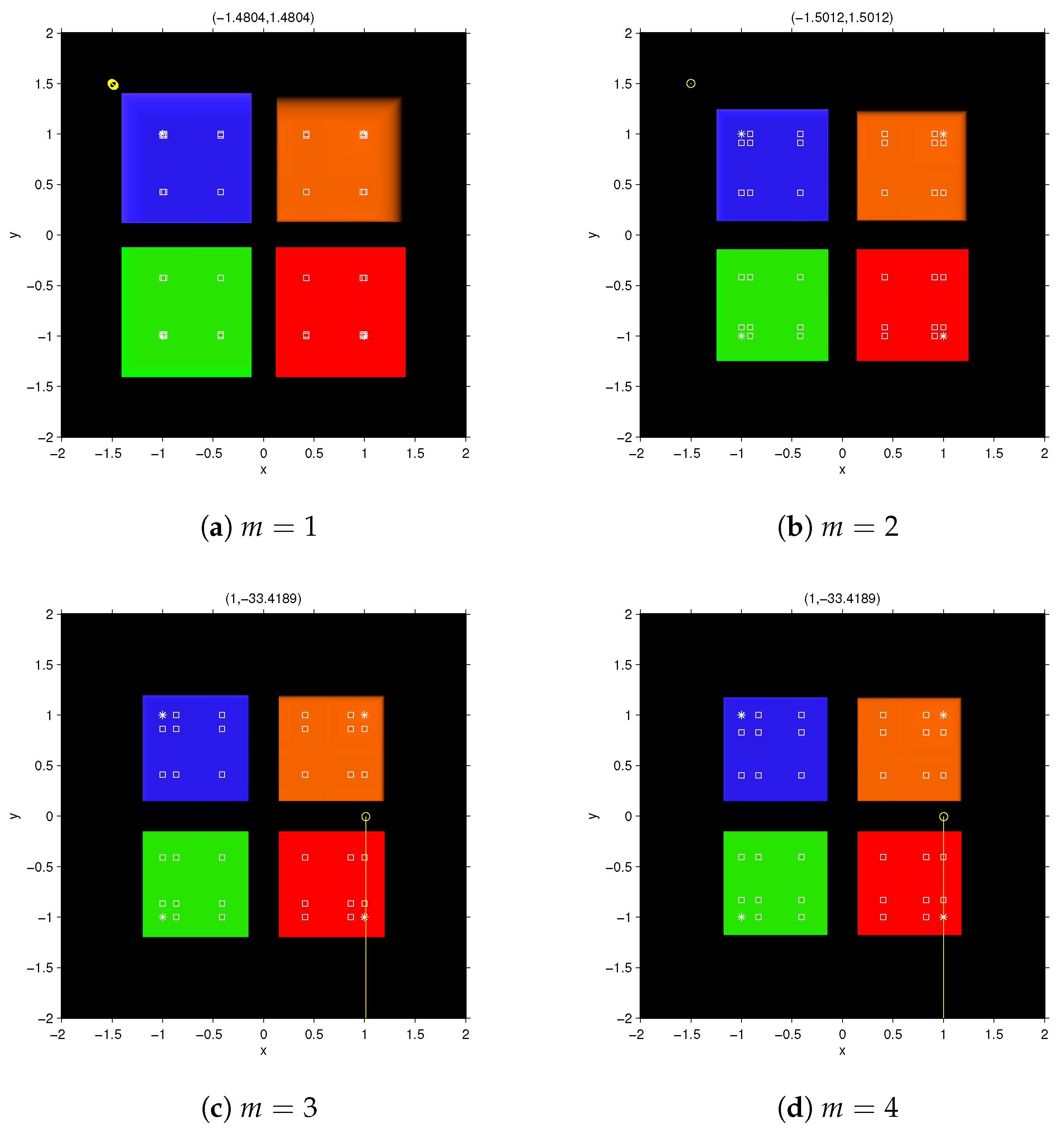
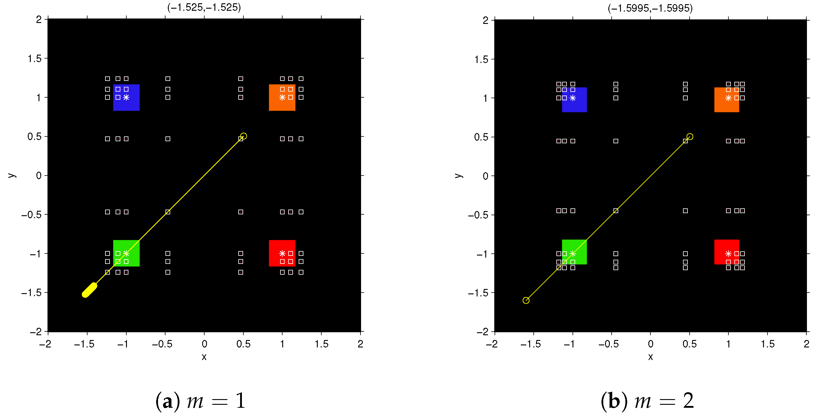
We use proposed families FMN_m, CMN_m and RMN_m on the polynomial systems $q\left(x\right)=0$, $r\left(x\right)=0$ and $p\left(x\right)=0$. In the following sections, the coordinate functions of the different classes of iterative methods, joint with their fixed and critical points are summarized.

2.1. Second-Degree Polynomial System $q\left(x\right)=0$

Proposition 2.

The coordinate functions of the fixed point operator ${\lambda }^{1,m}\left(x\right)$ associated to FMN_m for $m=1,2,\dots$ on polynomial system $q\left(x\right)=0$ are

$$\begin{array}{c}\hfill {\lambda }_j^{1,m}\left(x\right)=x_j-\frac{q_j\left(x\right)}{2x_j+q_j{\left(x\right)}^m},j=1,2.\end{array}$$

Moreover,

(a) 

For $m=1,2,\dots$, the only fixed points are the roots of $q\left(x\right)$, $(-1,-1)$, $(-1,1)$, $(1,-1)$ and $(1,1)$, that are also superattracting. There is no strange fixed point in this case.

(b) 

The components of free critical points $c_{{\lambda }^{1,m}}^n=(k,l)$ are roots of $2q_j\left(x\right)+(2+2m)x_j{q}_j{\left(x\right)}^m+q_j{\left(x\right)}^{\left(2m\right)}=0$, provided that k and l are not equal to 1 and $-1$, simultaneously.

Remark 1.

Except for $m=1$, that is a case with 12 free critical points, for $m>1$ there exist 32 free critical points of the fixed point operator associated to FMN_m. In particular, free critical points for the fixed point function ${\lambda }^{1,m}\left(x\right)$, $m=1,2,\dots ,6$ are

$$\begin{array}{c}(k,l),k,l\in \{-3.73205,-0.267949,-1,1\},\mathrm{for}m=1,\hfill \\ (k,l),k,l\in \{-2.11724,-1.13867,0.191305,0.760289,1,-1\},\mathrm{for}m=2,\hfill \\ (k,l),k,l\in \{-1.85429,-1.2072,-0.614069,-0.14308,1,-1\},\mathrm{for}m=3,\hfill \\ (k,l),k,l\in \{-1.74245,-1.24306,0.112834,0.541487,-1,1\},\mathrm{for}m=4,\hfill \\ (k,l),k,l\in \{-1.67929,-1.26615,-0.496325,-0.0927087,1,-1\},\mathrm{for}m=5,\hfill \\ (k,l),k,l\in \{-1.63822,-1.28266,0.0785163,0.464271,1,-1\},\mathrm{for}m=6,\hfill \end{array}$$

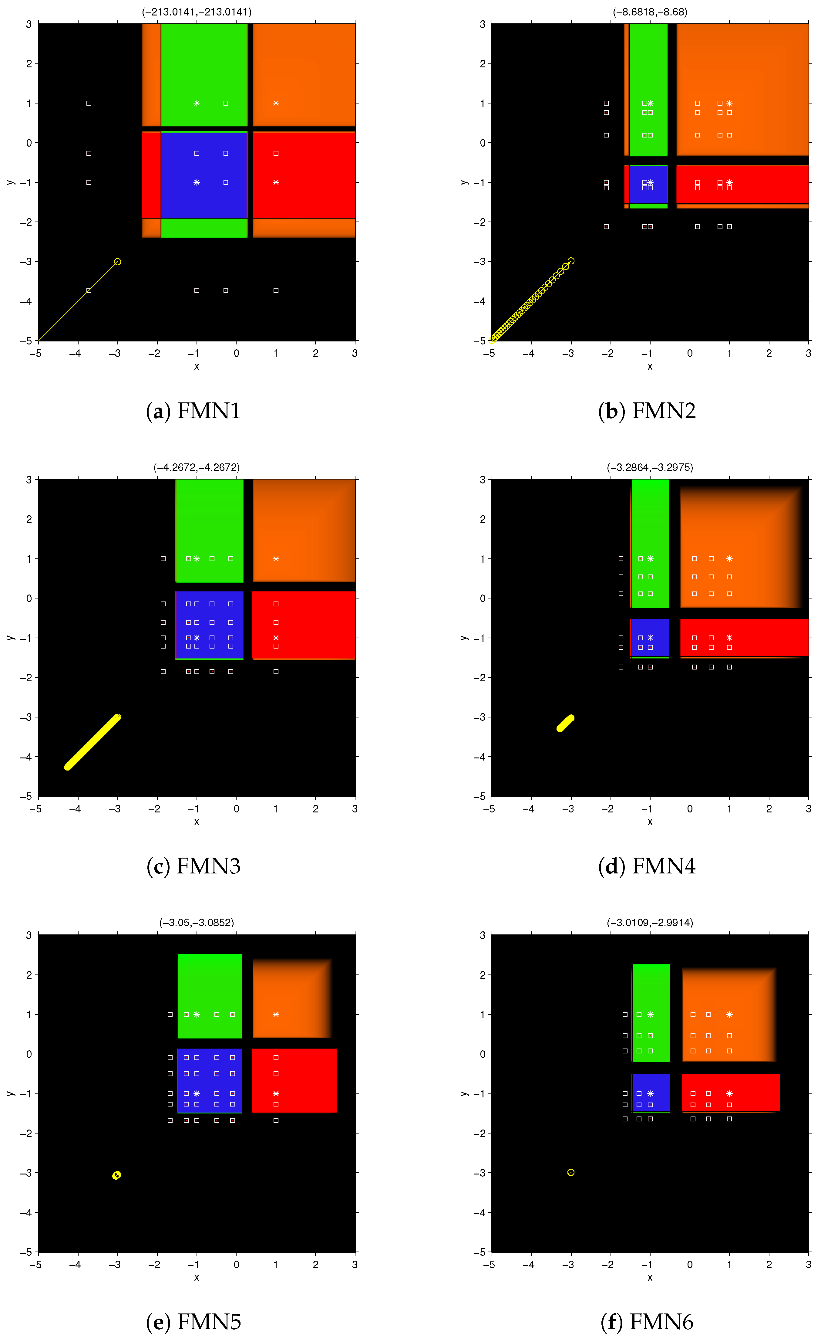
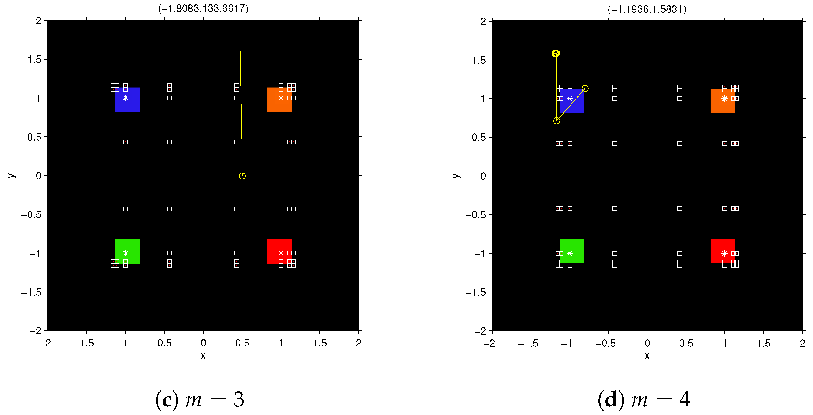
provided that k and l are not equal to 1 and $-1$, simultaneously.

Figure 1 shows the dynamical behavior of fixed point function ${\lambda }^{1,m}\left(x\right)$ for $m=1,2,\dots ,6$. These figures have been obtained by the routines described in [16]. To draw them, a mesh of $400\times 400$ points has been used, 200 was the maximum number of iterations involved and ${10}^{-3}$ the tolerance used as stopping criterium. In this paper, we have used a white star to show the roots of the nonlinear polynomial system and a white square for the free critical points. Figure 1 shows that, as greater m is, the wideness of basins of attraction decreases, in spite of having a better approximation of the Jacobian matrix. The color assigned to each of the basin of attraction corresponds to one of the roots of the nonlinear system. The black area shows the no convergence in the maximum number of iterations, or divergence.

Figure 1. Dynamical plane for FMN_m, $m=1,2,\dots ,6$ on $q\left(x\right)$. Green, orange, red and blue areas are the basins of attraction of the roots of $q\left(x\right)$ (marked as white stars); black area denotes divergence and white squares are free critical points.

To see the behavior of the vectorial function in the black area of dynamical planes, we visualize the orbit of the rational function corresponding to the starting point $(-3,-3)$ after 200 iterations. This orbit appears as a yellow circle per each iterate and yellow lines between each pair of consecutive iterates. In Figure 1a, corresponding to $m=1$, its value in the 200th iteration is $(-213.0141,-213.0141)$. Figure 1b, which corresponds to $m=2$, shows lower rate of divergence (or convergence to infinity), being its value at the 200th iteration $(-8.6818,-8.6818)$. This effect is higher by increasing m but, for $m\ge 3$ it is observed that

$$\frac{\parallel {\lambda }^{1,m}\left(x^{\left(0\right)}\right)-{\lambda }^{1,m}\left(x^{\left(200\right)}\right)\parallel }{\parallel {\lambda }^{1,m+1}\left(x^{\left(0\right)}\right)-{\lambda }^{1,m+1}\left(x^{\left(200\right)}\right)\parallel }\approx 1.$$

The vectors on the top of Figure 1c–f, corresponds to the last iterate with the starting point $x^{\left(0\right)}=(-3,-3)$.

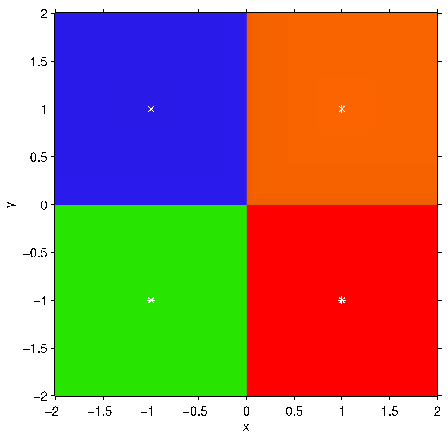
Proposition 3.

The coordinates of the fixed point operator ${\lambda }^{2,m}\left(x\right)$ associated to CMN_m, for $m=1,2,\dots$, and RMN_m, for $m=1,2,\dots$, on polynomial system $q\left(x\right)=0$ are

$$\begin{array}{c}\hfill {\lambda }_j^2\left(x\right)=\frac{1+x_j^2}{2x_j},j=1,2,\end{array}$$

which are the same components of the fixed point function of Newton’s method on $q\left(x\right)$.

Since $q\left(x\right)$ is a 2nd-degree polynomial system, the approximations of order equal or higher than 2 of Jacobian matrix are exact and the fixed point function of the CMN_m and RMN_m methods coincide with that of Newton’s method. In this case, $(-1,-1)$, $(-1,1)$, $(1,-1)$ and $(1,1)$ are superattracting fixed points and there are no strange fixed points or free critical points. Figure 2 shows the resulting dynamical plane, that coincides with that of Newton’s method.

Figure 2. Dynamical plane of CMN_m, RMN_m and Newton’s method on $q\left(x\right)$. Green, orange, red and blue areas are the basins of attraction of the roots of $q\left(x\right)$ (marked as white stars).

2.2. Sixth-Degree Polynomial System $r\left(x\right)=0$

The corresponding results about FMN_m, CMN_m and RMN_m classes applied on sixth-degree polynomial system $r\left(x\right)=0$ are summarized in the following propositions. They resume, in each case, the iteration function, the fixed and critical points.

Proposition 4.

The coordinate functions of the fixed point operator $h^{1,m}\left(x\right)$ associated to FMN_m on $r\left(x\right)$, for $m=1,2,\dots$, are

$$\begin{array}{c}\hfill h_j^{1,m}\left(x\right)=x_j-\frac{r_j{\left(x\right)}^{1+m}}{-x_j^6+{(x_j+r_j{\left(x\right)}^m)}^6},j=1,2.\end{array}$$

Moreover,

(a) 

For $m\ge 1$ the fixed points are $(-1,-1)$, $(-1,1)$, $(1,-1)$ and $(1,1)$ that are also superattracting. There are no strange fixed points in this case.

(b) 

The coordinates of free critical points $c_{h^{1,m}}^n=(k,l)$ are the roots of the polynomial

$$\begin{array}{ccc}\hfill {(x_j^6-{(x_j+r_j{\left(x\right)}^m)}^6)}^2& +& r_j{\left(x\right)}^{1+m}(-6x_j^5+6(1+6m{x}_j^5{r}_j{\left(x\right)}^{-1+m}){(x_j+r_j{\left(x\right)}^m)}^5)\hfill \\ & +& 6(1+m)x_j^5{r}_j{\left(x\right)}^m(x_j^6-{(x_j+r_j{\left(x\right)}^m)}^6),\hfill \end{array}$$

for $j=1,2$ and $m=1,2,\dots$, provided that k and l are not equal to $-1$ and 1 simultaneously.

Remark 2.

Except for $m=1$, in which case that the fixed point function $h^{1,m}\left(x\right)$ has 12 free critical points, the multidimensional rational function FMN_m, for $m=2,3,\dots$, has 32 free critical points. The free critical points in this case are

$$\begin{array}{c}(k,l),k,l\in \{-1.3191,-0.290716,-1,1\}\mathrm{for}m=1,\hfill \\ (k,l),k,l\in \{-1.20592,-1.01655,0.289432,0.978576,-1,1\}\mathrm{for}m=2,\hfill \\ (k,l),k,l\in \{-1.17593,-1.03983,-0.934077,-0.288186,-1,1\}\mathrm{for}m=3,\hfill \\ (k,l),k,l\in \{-1.16205,-1.0543,0.286976,0.897504,-1,1\}\mathrm{for}m=4,\hfill \\ (k,l),k,l\in \{-1.15401,-1.064,-0.868592,-0.285801,-1,1\}\mathrm{for}m=5,\hfill \\ (k,l),k,l\in \{-1.14876,-1.07101,0.284659,0.845166,-1,1\}\mathrm{for}m=6,\hfill \end{array}$$

provided that k and l are not equal to $-1$ and 1 simultaneously.

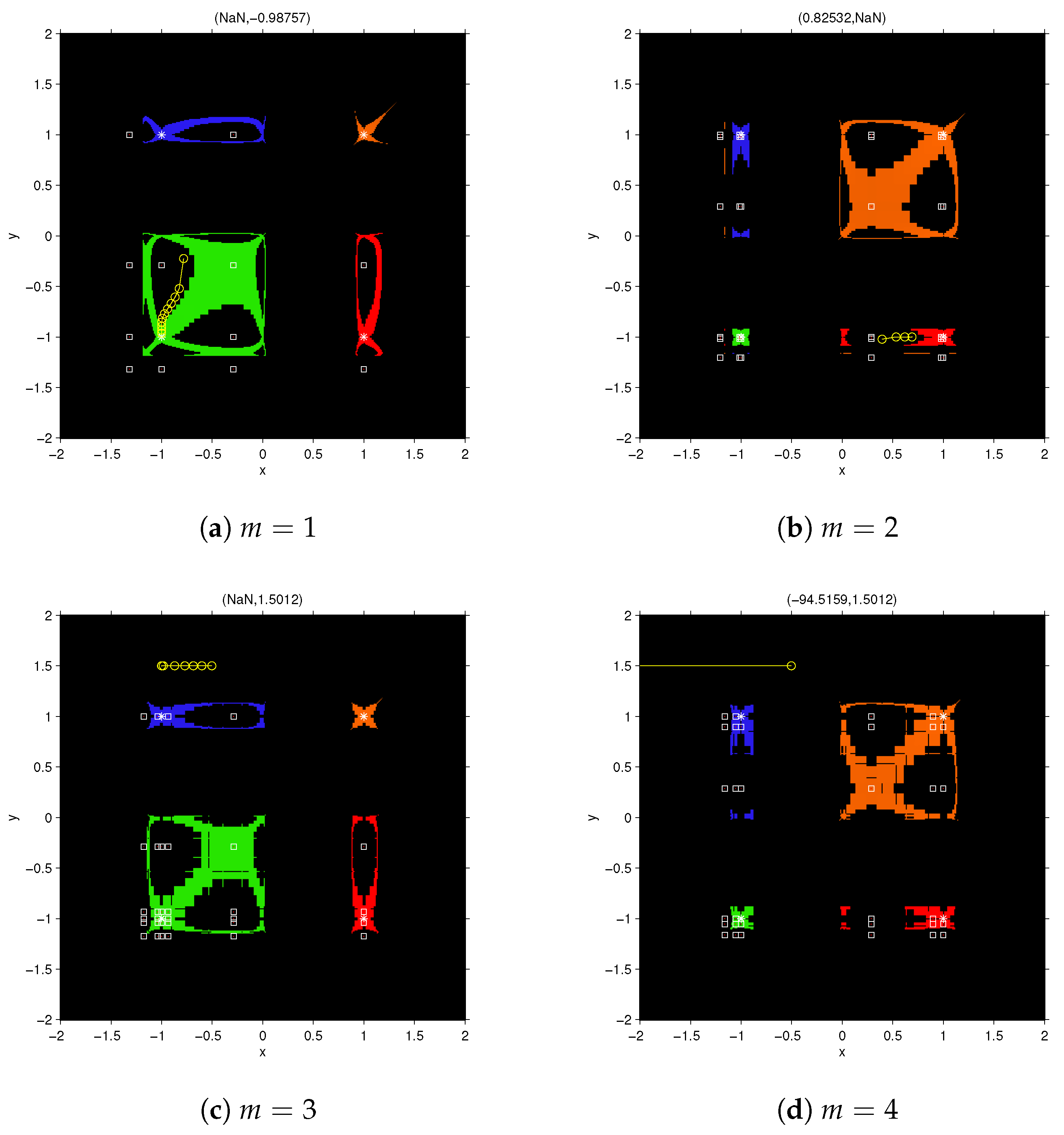
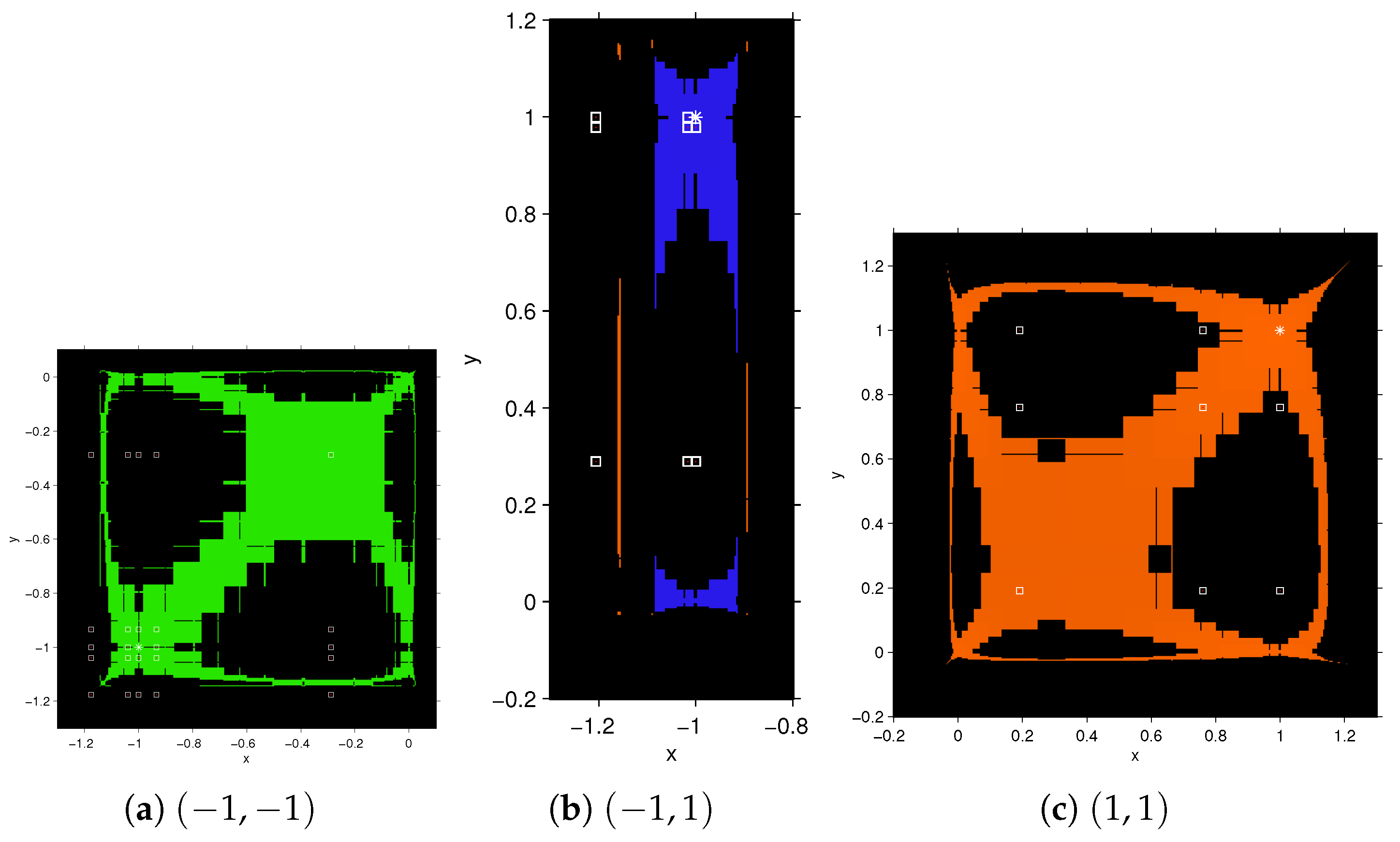
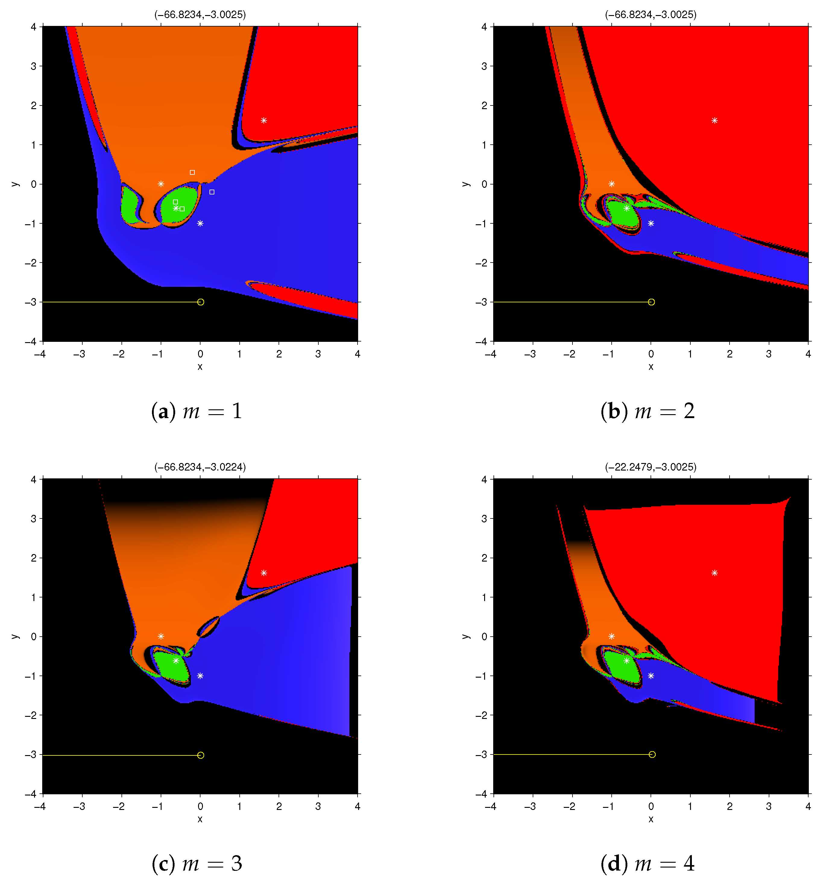
Figure 3 shows the dynamical planes of the fixed point function $h^{1,m}\left(x\right)$ for $m=1,2,\dots ,6$. Inside the black areas, there are regions where the orbits tend toward the poles of the rational function (those points that make the denominator of the elements of the rational function null). In fact, the orbits of points in these areas reach very close to the roots, so the vectorial rational function at these points become numerically singular. Figure 3a,b show two points in these black areas.

Figure 3. Dynamical plane of FMN_m method for $m=1,2,\dots ,6$ on $r\left(x\right)$. Green, orange, red and blue areas are the basins of attraction of the roots of $q\left(x\right)$ (marked as white stars); black area denotes divergence and white squares are free critical points.

Figure 4 and Figure 5 show details of the dynamical planes of FMN₂ and FMN₃ methods. These figures show the difference between the basins of attraction of an odd member with an even member of the family FMN_m. Because of the symmetry, the transpose of the basin of attraction of $(1,-1)$ coincide with that of $(-1,1)$, so we only depicted one of them.

Figure 4. Basins of attraction of $(-1,-1)$, $(-1,1)$ and $(1,1)$ for FMN₂ method on $r\left(x\right)$. Green, orange, red and blue areas are the basins of attraction of the roots of $q\left(x\right)$ (marked as white stars); black area denotes divergence and white squares are free critical points.

Figure 5. Basins of attraction of $(-1,-1)$, $(1,-1)$ and $(1,1)$ for FMN₃ method on $r\left(x\right)$. Green, orange, red and blue areas are the basins of attraction of the roots of $q\left(x\right)$ (marked as white stars); black area denotes divergence and white squares are free critical points.

The analysis for the cases of central divided differences is made in the following result.

Proposition 5.

The coordinate functions of the fixed point operator $h^{2,m}\left(x\right)$ associated to CMN_m, for $m=1,2,\dots$, on $r\left(x\right)$ are

$$\begin{array}{c}\hfill h_j^{2,m}\left(x\right)=x_j-\frac{r_j\left(x\right)}{6x_j^5+20x_j^3{r}_j{\left(x\right)}^{2m}+6x_j{r}_j{\left(x\right)}^{4m}},j=1,2.\end{array}$$

Moreover,

(a) 

The fixed points are $(-1,-1)$, $(1,-1)$, $(-1,1)$ and $(1,1)$ that are also superattracting and there are not strange fixed points.

(b) 

The components of free critical points $c_{h^{2,m}}^n=(k,l)$ in this case are the roots of the polynomial $P_{h^{2,m}}^j\left(x\right)$, provided that $Q_{h^{2,m}}^j\ne 0$, being

$$\begin{array}{ccc}{P}_{h^{2,m}}^j\left(x\right)\hfill & =& 15x_j^{10}+30(3+4m)x_j^8{r}_j{\left(x\right)}^{2m}-3r_j{\left(x\right)}^{4m}+(221+72m)x_j^6{r}_j{\left(x\right)}^{4m}\hfill \\ & & +6x_j^2{r}_j{\left(x\right)}^{2m}(-5+3r_j{\left(x\right)}^{6m})+15x_j^4(-1+8r_j{\left(x\right)}^{6m}),j=1,2,\hfill \\ \hfill Q_{h^{2,m}}^j& =& 2{(3x_j^5+10x_j^3{r}_j{\left(x\right)}^{2m}+3x_j{r}_j{\left(x\right)}^{4m})}^2,j=1,2,\hfill \end{array}$$

where k and l are not simultaneously equal to 1 and $-1$.

Remark 3.

The fixed point rational function $h^{2,m}\left(x\right)$, for all m, has 32 free critical points. The free critical points in this case are

$$\begin{array}{c}(k,l),k,l\in \{-0.424661,0.424661,-0.984594,0.984594,1,-1\}\mathrm{for}m=1.\hfill \\ (k,l),k,l\in \{-0.417373,0.417373,-0.913322,0.913322,1,-1\}\mathrm{for}m=2.\hfill \\ (k,l),k,l\in \{-0.410772,0.410772,-0.864585,0.864585,1,-1\}\mathrm{for}m=3.\hfill \\ (k,l),k,l\in \{-0.404767,0.404767,-0.830398,0.830398,-1,1\}\mathrm{for}m=4.\hfill \\ (k,l),k,l\in \{-0.399279,0.399279,-0.804535,0.804535,1,-1\}\mathrm{for}m=5.\hfill \\ (k,l),k,l\in \{-0.394237,0.394237,-0.783908,0.783908,1,-1\}\mathrm{for}m=6.\hfill \end{array}$$

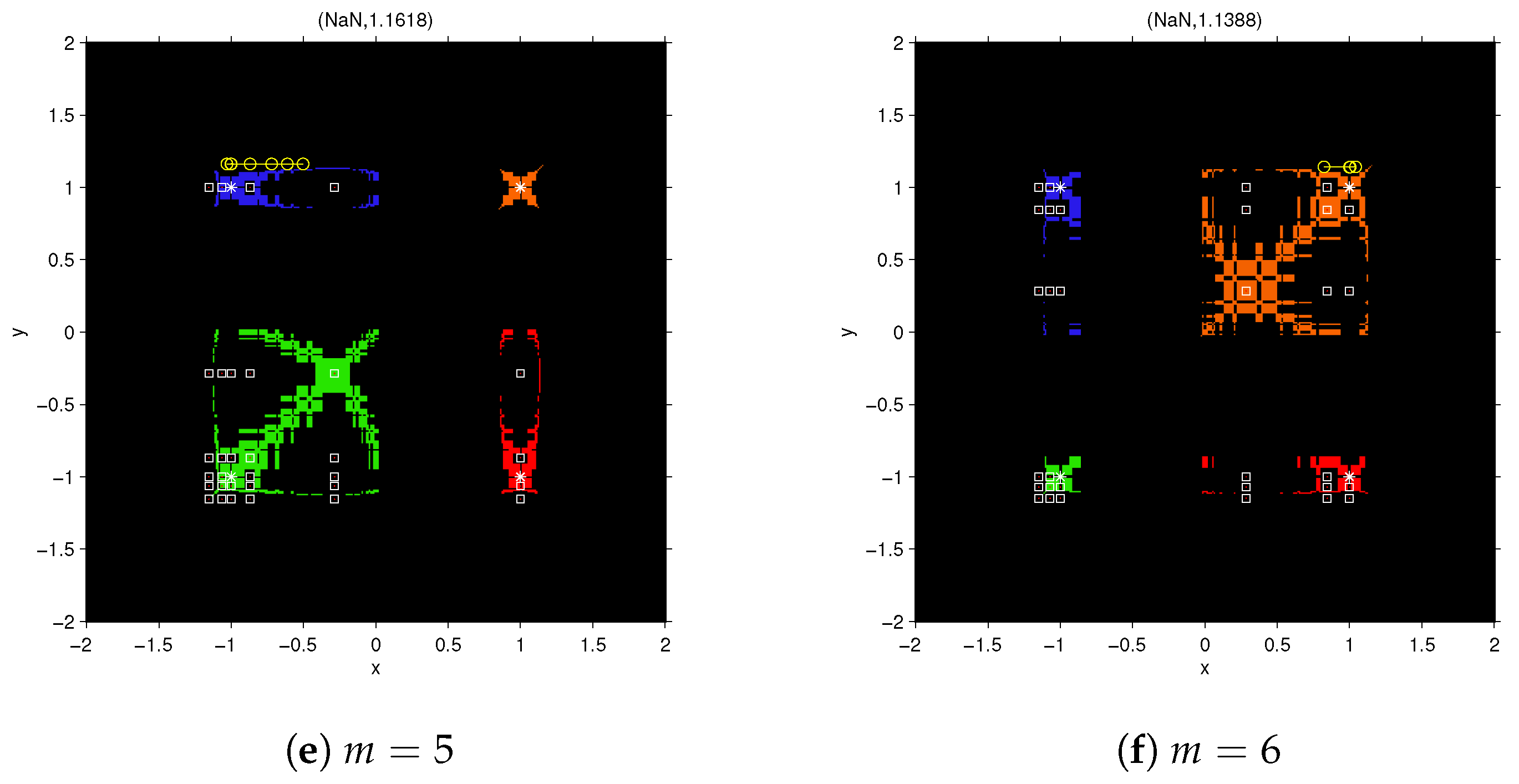
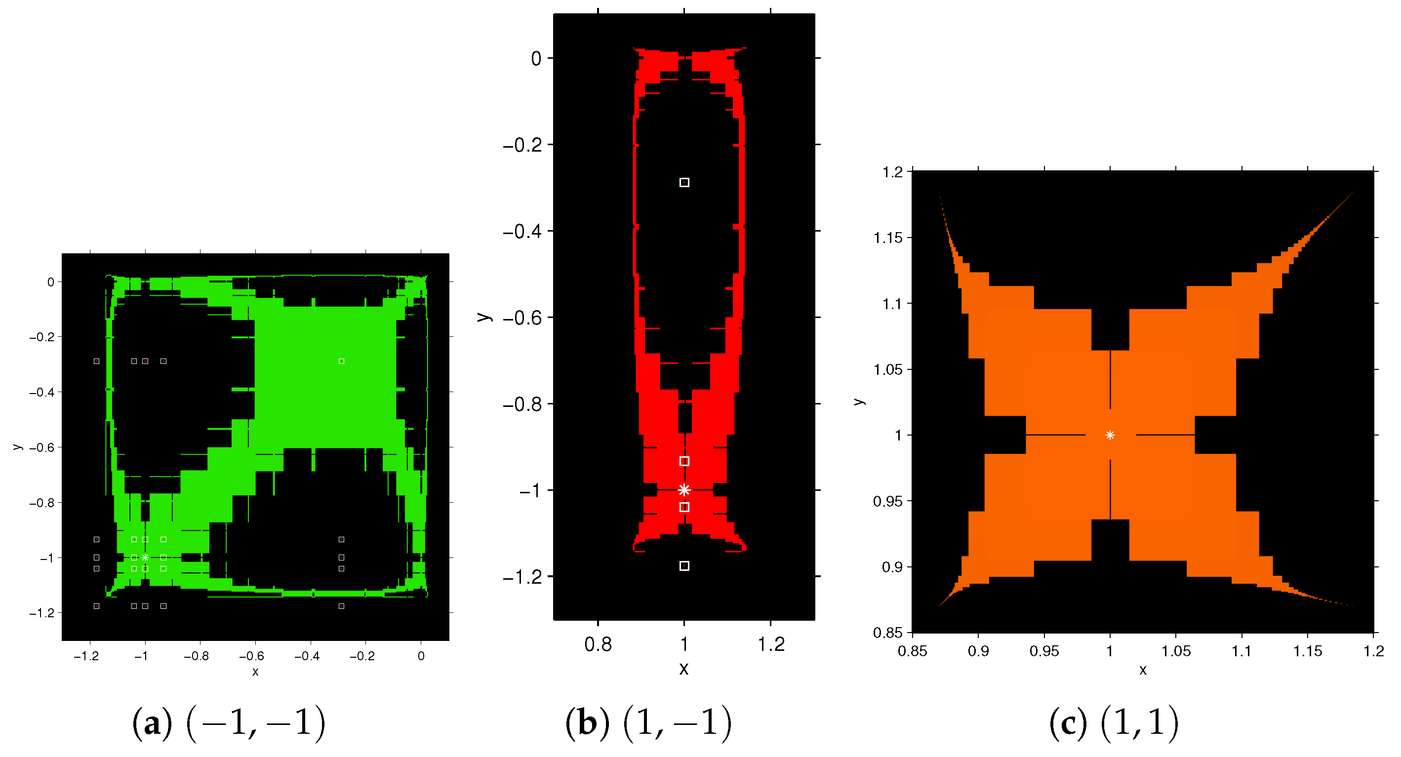
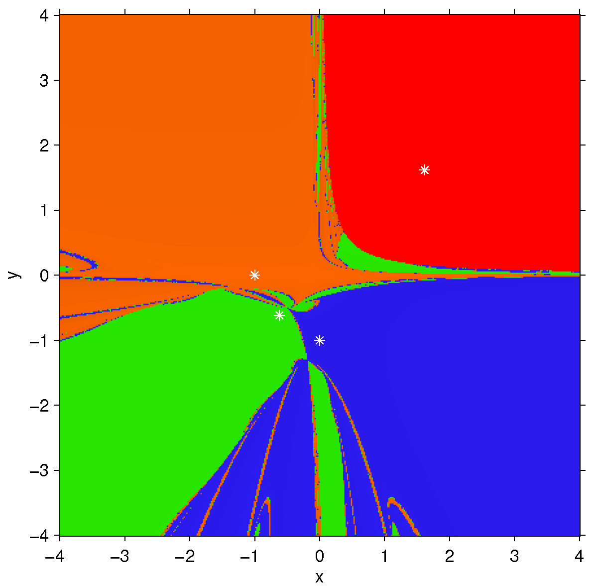
provided that k and l are not equal to 1 and $-1$ simultaneously.

Central divided differences show very stable behavior. All the free critical points are inside the basins of attraction of the roots. This means that it is not possible other performance than convergence to the roots (or divergence). In fact, the basins of attraction of the roots in this case are much greater than those in the forward divided difference. Black areas near to the boundaries of the basins of attraction are regions of slow convergence or divergence. Figure 6a,b shows the slow convergence of the point $(-1.5,1.5)$ towards (−1,1); let us observe that, as for $m=1$ point $(-1.5,1.5)$ is closer to the boundary so its speed is higher than that for $m=2$. The behavior of function $h^{2,m}\left(x\right)$ in black area among the basins of attraction and near the axis x and y are similar for $m=1,2,\dots$. In fact by choosing points in this area the iterative function is slowly divergent (see Figure 6c,d).

Figure 6. Dynamical plane for CMN_m method, $m=1,2,3,4$ on $r\left(x\right)$. Green, orange, red and blue areas are the basins of attraction of the roots of $q\left(x\right)$ (marked as white stars); black area denotes divergence and white squares are free critical points.

Let us remark that, although this scheme is quite stable, the basins of attraction of the roots are much smaller than those of Newton’s method on $r\left(x\right)$, where there are not black regions.

Finally, the following result gives us information about the stability of the sixth-degree system when higher-order estimations of the Jacobian are made.

Proposition 6.

The coordinate functions of the fixed point operator $h^{3,m}\left(x\right)$ associated to RMN_m on $r\left(x\right)$, for $m=1,2,\dots$, are

$$\begin{array}{c}\hfill h_j^{3,m}\left(x\right)=x_j-\frac{2r_j\left(x\right)}{12x_j^5-3x_j{r}_j{\left(x\right)}^{4m}},j=1,2.\end{array}$$

(a) 

For $m=1,2,\dots$, the fixed points are $(-1,-1)$, $(-1,1)$, $(1,-1)$ and $(1,1)$ that are also superattracting and there are not strange fixed points in this case.

(b) 

The components of free critical points $c_{h^{3,m}}^n=(k,l)$ are the roots of polynomial

$$\begin{array}{c}\hfill P_{h^{3,m}}^j\left(x\right)=-40x_j^4+40x_j^{10}+2r_j{\left(x\right)}^{4m}-2(7+24m)x_j^6{r}_j{\left(x\right)}^{4m}+3x_j^2{r}_j{\left(x\right)}^{8m},\end{array}$$

for $j=1,2$ and $m=1,2,\dots$, provided that $-4x_j^5+x_j{r}_j{\left(x\right)}^{4m}\ne 0$ and k and l are not simultaneously equal to 1 and $-1$.

Remark 4.

The fixed point function $h^{3,m}\left(x\right)$ on $r\left(x\right)$ for all m has 60 free critical points. The free critical points, for $m=1,2,\dots ,6$, are

$$\begin{array}{c}(k,l),k,l\in \{-0.467908,0.467908,-1.1047,1.1047,-1.23916,1.23916,-1,1\}\mathrm{for}m=1,\hfill \\ (k,l),k,l\in \{-0.446836,0.446836,-1.10721,1.10721,-1.18013,1.18013,-1,1\}\mathrm{for}m=2,\hfill \\ (k,l),k,l\in \{-0.431784,0.431784,-1.16201,1.16201,-1.10964,1.10964,-1,1\}\mathrm{for}m=3,\hfill \\ (k,l),k,l\in \{-0.420071,0.420071,-1.15298,1.15298,-1.11137,1.11137,-1,1\}\mathrm{for}m=4,\hfill \\ (k,l),k,l\in \{-0.41049,0.41049,-1.1475,1.1475,-1.11265,1.11265,-1,1\}\mathrm{for}m=5,\hfill \\ (k,l),k,l\in \{-0.402394,0.402394,-1.14379,1.14379,-1.11364,1.11364,-1,1\}\mathrm{for}m=6,\hfill \end{array}$$

provided that k and l are not equal to 1 and $-1$, simultaneously.

In this case, we obtain approximations of order $4,8,12,\dots$ for $m=1,2,3,\dots$, respectively, but nevertheless their basins of attraction are smaller than those of central divided difference (and of course of Newton’s method). Figure 7 shows the dynamical planes for $m=1,2,3,4$. As in the previous cases, in the black area the convergence is very slow (or it diverges).

Figure 7. Dynamical plane for RMN_m method, $m=1,2,3,4$ on $r\left(x\right)$. Green, orange, red and blue areas are the basins of attraction of the roots of $q\left(x\right)$ (marked as white stars); black area denotes divergence and white squares are free critical points.

2.3. Second-Degree Polynomial System $p\left(x\right)=0$

The results about FMN_m, CMN_m and RMN_m classes applied on second-degree polynomial system $p\left(x\right)=0$ are stated in the following propositions. They resume, in each case, the iteration function, the fixed and critical points.

Proposition 7.

The coordinate functions of the fixed point operator $k^{1,m}\left(x\right)$ associated to FMN_m on $p\left(x\right)$, for $m=1,2,\dots$, are

$$\begin{array}{c}\hfill k_1^{1,m}\left(x\right)=x_1-\frac{-1-x_1+x_2^2}{-1+\frac{(-x_1^2+{(x_1+{(1-x_1^2+x_2)}^m)}^2)(-x_2^2+{(x_2+{(1+x_1-x_2^2)}^m)}^2)}{{(1-x_1^2+x_2)}^m{(1+x_1-x_2^2)}^m}}\\ \hfill -\frac{(-1+x_1^2-x_2)(-x_2^2+{(x_2+{(1+x_1-x_2^2)}^m)}^2)}{{(1+x_1-x_2^2)}^m(-1+\frac{(-x_1^2+{(x_1+{(1-x_1^2+x_2)}^m)}^2)(-x_2^2+{(x_2+{(1+x_1-x_2^2)}^m)}^2)}{{(1-x_1^2+x_2)}^m{(1+x_1-x_2^2)}^m})},m=1,2,\cdots \\ \hfill k_2^{1,m}\left(x\right)=x_2-\frac{-1+x_1^2-x_2}{-1+\frac{(-x_1^2+{(x_1+{(1-x_1^2+x_2)}^m)}^2)(-x_2^2+{(x_2+{(1+x_1-x_2^2)}^m)}^2)}{{(1-x_1^2+x_2)}^m{(1+x_1-x_2^2)}^m}}\\ \hfill -\frac{(-1-x_1+x_2^2)(-x_1^2+{(x_1+{(1-x_1^2+x_2)}^m)}^2)}{{(1-x_1^2+x_2)}^m(-1+\frac{(-x_1^2+{(x_1+{(1-x_1^2+x_2)}^m)}^2)(-x_2^2+{(x_2+{(1+x_1-x_2^2)}^m)}^2)}{{(1-x_1^2+x_2)}^m{(1+x_1-x_2^2)}^m})},m=1,2,\cdots .\end{array}$$

Moreover,

(a) 

For $m\ge 1$ the only fixed points are the roots $(-1,0)$, $(0,-1)$, $\left(\frac{1}{2}\left(1-\sqrt{5}\right),\frac{1}{2}\left(1-\sqrt{5}\right)\right)$ and $\left(\frac{1}{2}\left(1+\sqrt{5}\right),\frac{1}{2}\left(1+\sqrt{5}\right)\right)$, that are superattracting.

(b) 

For $m=1$, the free critical points are $(-0.632026,-0.460233)$, $(-0.460233,-0.632026)$, $(-0.203287,0.294659)$ and $(0.294659,-0.203287)$.

The calculation of free critical points of $k^{1,m}\left(x\right)$ for $m>1$ is very complicated hence, so it has been provided only for $m=1$. Figure 8 shows the dynamical planes of the fixed point function $k^{1,m}\left(x\right)$ for $m=1,2,3,4$. Similar results to polynomial system $q\left(x\right)=0$ and $r\left(x\right)=0$ have been obtained in this case, as by increasing m, the wideness of the basins of attraction decreases. To study the behavior of the vectorial function in the black area of dynamical planes, we visualize the diverging orbits of $k^{1,m}\left(x\right)$ with the starting point $(0,-3)$, after 200 iterations. The vectors on the top of the Figure 8a–d, show the last vectorial iterate with the starting point $(0,-3)$.

Figure 8. Dynamical plane for FMN_m method, $m=1,2,3,4$ on $p\left(x\right)$. Green, orange, red and blue areas are the basins of attraction of the roots of $q\left(x\right)$ (marked as white stars); black area denotes divergence and white squares are free critical points.

The following proposition shows, that using CMN_m, for $m=1,2,\dots$, and RMN_m, for $m=1,2,\dots$, on polynomial system $p\left(x\right)=0$, we obtain, as was the case for the system $q\left(x\right)=0$, the same fixed point function as the classical Newton’s method.

Proposition 8.

The coordinates of the fixed point operator $k^{2,m}\left(x\right)$ (which is denoted by $k^2\left(x\right)$) associated to CMN_m for $m=1,2,\dots$ and RMN_m for $m=1,2,\dots$ on polynomial system $p\left(x\right)$ are

$$\begin{array}{c}\hfill k_1^2\left(x\right)=\frac{1+2(1+x_1^2)x_2+x_2^2}{-1+4x_{1}4x_2},\\ \hfill k_2^2\left(x\right)=\frac{1+x_1^2+2x_1(1+x_2^2)}{-1+4x_{1}4x_2},\end{array}$$

which are the same components of the fixed point function of Newton’s method on $p\left(x\right)$. Moreover, the fixed points of $k^2\left(x\right)$ are the roots $(-1,0)$, $(0,-1)$, $\left(\frac{1}{2}\left(1-\sqrt{5}\right),\frac{1}{2}\left(1-\sqrt{5}\right)\right)$ and $\left(\frac{1}{2}\left(1+\sqrt{5}\right),\frac{1}{2}\left(1+\sqrt{5}\right)\right)$ that are superattracting. There are no strange fixed points nor free critical points in this case.

Figure 9 shows the dynamical plane of the fixed point function $k^2\left(x\right)$, corresponding to methods CMN_m and RMN_m for any $m=1,2,\dots$ as well as their original partner, Newton’s scheme.

Figure 9. Dynamical plane of CMN_m, RMN_m and Newton’s method on $p\left(x\right)$. Green, orange, red and blue areas are the basins of attraction of the roots of $q\left(x\right)$ (marked as white stars); black area denotes divergence and white squares are free critical points.

3. Conclusions

In this paper, several new Jacobian-free Newton’s method have been introduced, by using forward, central and Richardson divided differences based on an element-by-element power of the nonlinear function $F\left(x\right)$, $G\left(x\right)={(f_1{\left(x\right)}^m,f_2{\left(x\right)}^m,\dots ,f_n{\left(x\right)}^m)}^T$. As far as we know, these Jacobian-free variants of Newton’s method have not been analyzed until now. We conclude that better estimations do not always involve greater stability. In fact, the best scheme in terms of numerical efficiency and wideness of the sets of converging initial points, is CMN_m. This central differences method does not need to calculate and evaluate the Jacobian matrix as Newton’s method and provides similar basins of attraction. Although Richardson’s method reaches good results of convergence, has a computational cost that discourages its use.