Article

Image Deblurring under Impulse Noise via Total Generalized Variation and Non-Convex Shrinkage

School of Physics and Information Engineering, Key Lab of Intelligent Optimization and Information Processing, Minnan Normal University, Zhangzhou 363000, China
*
Author to whom correspondence should be addressed.
Algorithms 2019, 12(10), 221; https://doi.org/10.3390/a12100221
Submission received: 17 September 2019 / Revised: 16 October 2019 / Accepted: 21 October 2019 / Published: 22 October 2019

Abstract

:
Image deblurring under the background of impulse noise is a typically ill-posed inverse problem which attracted great attention in the fields of image processing and computer vision. The fast total variation deconvolution (FTVd) algorithm proved to be an effective way to solve this problem. However, it only considers sparsity of the first-order total variation, resulting in staircase artefacts. The L1 norm is adopted in the FTVd model to depict the sparsity of the impulse noise, while the L1 norm has limited capacity of depicting it. To overcome this limitation, we present a new algorithm based on the Lp-pseudo-norm and total generalized variation (TGV) regularization. The TGV regularization puts sparse constraints on both the first-order and second-order gradients of the image, effectively preserving the image edge while relieving undesirable artefacts. The Lp-pseudo-norm constraint is employed to replace the L1 norm constraint to depict the sparsity of the impulse noise more precisely. The alternating direction method of multipliers is adopted to solve the proposed model. In the numerical experiments, the proposed algorithm is compared with some state-of-the-art algorithms in terms of peak signal-to-noise ratio (PSNR), structural similarity (SSIM), signal-to-noise ratio (SNR), operation time, and visual effects to verify its superiority.

1. Introduction

Image deblurring under impulse noise is important in digital image processing research. It is widely applied in many aspects of science and engineering such as space detection, photodetection, remote sensing technology, medical image analysis, and geological exploration. In the process of acquiring, storing, and transmitting images, owing to limitations of imaging equipment and conditions, images are prone to quality degradation, such as image blurring, noise pollution, contrast decline, and loss of details. Image restoration of degraded images is an inverse problem whose solution is often ill-posed [1]. For such types of problems, regularization proved to be an effective method. This involves the proper use of some prior information of the degraded image as a fidelity term and an image optimization model that contains an efficient solution algorithm as a regularization term, because recovering a clear image is of great importance for advanced image processing in the later stages.
The total variation (TV) regularization proposed by Rudin, Osher, and Fatemi [2], also known as the ROF model, proved to be one of the most advanced regularizations in the field of image reconstruction. Based on the TV regularization, some extended models and their algorithms were widely applied to image restoration. For example, Wang et al. [3] proposed a fast total variation deconvolution (FTVd) model for image deblurring. The model uses the total variation (TV) regularization based on the assumption that the image is piecewise smooth; the method can remove image noise sufficiently, but it is prone to producing a “staircase effect”. Furthermore, the FTVd model adopted the L1 norm to express the sparsity of impulse noise. However, it cannot depict the statistic characteristics of impulse noise.
Recently, some TV extensions emerged. Sakurai et al. [4] proposed a four-directional total variation model to extend the vertical and horizontal gradient information in the TV regularization into four directions. Ren et al. [5] proposed a fractional-order TV (FTV) model and tried to extend the integer-order TV model to the fractional order. Selesnick and Chen [6] proposed an overlapping group sparsity TV (OGSTV) model, in which the neighborhood information of the image gradient was taken into account and applied in conjunction with an L2-norm fidelity term to the Gaussian-noise denoising of one-dimensional signals. Liu et al. [7] extended the model to a two-dimensional model based on an L1-norm fidelity term and applied the extended model to image deconvolution and impulse noise removal, achieving good results [8]. Bredies et al. [9] proposed a total generalized variation (TGV) model based on total variation, which simultaneously constrains the first-order and second-order gradients of the image and has many excellent mathematical properties such as convexity, lower semi-continuity, and rotation invariance; it is also capable of approximating any number of items. The TGV model proved—in theory and practice—to be able to remove the staircase effect effectively while preserving the edges and details of the image. TGV regularization terms attracted wide attention in the academic community and were applied to the reconstruction of nuclear magnetic resonance images [10] and seismic signal denoising [11,12]. Inspired by the advantages of TGV regularization, we incorporate it here in the image deblurring process.
The aforementioned image deblurring methods mostly employ the L1 norm to constrain the fidelity term. However, the L1 norm is a convex relaxation of the L0 norm, with limited ability to induce sparsity [13]. Recently, Woodworth and Chartrand [14] proved that Lp-pseudo-norm shrinkage is a method with better sparsity compared with soft-threshold shrinkage, which attracted extensive attention in academia. Zheng et al. [15] theoretically compared the advantages of Lp-minimization and L1-minimization, and tested them in a Gaussian noisy setting. Zhang et al. [16] applied Lp shrinkage [17] to the reconstruction of tomographic images to obtain an effect superior to the L1-norm constraint. Chen et al. [18] applied an Lp-pseudo-norm constraint to the sparse time–frequency representation of the seismic signal spectrum to obtain a time–frequency spectrum with higher time–frequency resolution. Wong et al. [19] proposed a model combining an Lp-pseudo-norm fidelity term and OGS regularization, which uses neighborhood structure similarity of image gradients for image denoising.
Considering the superiority of Lp-pseudo-norm and TGV, here, we employ Lp-pseudo-norm to describe the sparsity of impulse noise and adopt the TGV regularization term to fit the image sparsity. On the one hand, the Lp-pseudo-norm constraint increases the degrees of freedom of the fidelity term and better represents the sparsity of the impulse noise. In this way, the deblurring process is more robust to noise pollution. On the other hand, the TGV regularization term simultaneously puts constraints on the information of the first-order and second-order gradients of the image, thereby effectively suppressing the staircase effect.
To solve the problem, the alternating direction method of multipliers (ADMM) [20,21] is employed to decompose the complex problem into a number of sub-problems that are relatively easy to solve. At the same time, to improve the efficiency of the algorithm, it is assumed here that the image satisfies a periodic boundary condition. Following a fast deconvolution method [3,22,23], fast Fourier transform (FFT) is employed based on the convolution law to transform image differences in the time domain to differences in the frequency domain to avoid large matrix multiplication operations. In numerical experiments, the proposed new method is compared with FTVd, TGV, and OGSTV in terms of the following objective indicators: peak signal-to-noise ratio (PSNR), structural similarity (SSIM), signal-to-noise ratio (SNR), and computation time.
The rest of this paper is organized as follows: Section 2 presents prerequisite knowledge related to the algorithms used in this study, including the modeling of the TGV regularization term and the Lp norm. Section 3 firstly presents the model proposed in this study and then elaborates on an efficient method for solving the model in the ADMM framework. Results of the numerical experiment are presented in Section 4, and conclusions are given in Section 5.

2. Prerequisite Knowledge

2.1. FTVd Model

We assumed that the linear mathematical model of an observed degraded image is expressed as follows [24]:
G = H F + N .
For the sake of simplicity, it was assumed, in this study, that the processed image is an N × N square matrix, which can be easily generalized to an image of size M × N . G N × N is a degraded image matrix, F N × N represents an original unknown clear image matrix, H is a blur kernel matrix, represents the two-dimensional convolution operator, and N N × N represents additive noise, such as Gaussian noise and impulse noise. For impulse noise, a discrete ROF model is constructed using the L1 norm, where the FTVd model is expressed as
m i n F { H F G 1 + μ R ( F ) } ,
where · 1 represents the Euclidean L1 norm. In Equation (2), H F G 1 is the fidelity term using the L1-norm, and R ( F ) is the regularization. In FTVd mode, R ( F ) = K h F 1 + K v F v 1 is the anisotropic total variation (ATV) regularization term, K h = [ 1 , 1 ] and K v = [ 1 , 1 ] T are the horizontal and vertical convolution operators, respectively, and μ is a regularization parameter higher than zero, which serves to balance the fidelity term and the regularization term.
As is shown in Equation (1), FTVd employs the ATV as the regularization and the L1 norm to depict the sparsity of impulse noise. However, ATV assumes the processed image to be piecewise constant. As a result, staircase artefacts occur. In addition, the L1 norm is the convex relaxation of the L0 norm. It cannot express the sparsity of impulse noise precisely. Considering the disadvantages of FTVd, the TGV regularization is employed to replace the ATV regularization, and the Lp-pseudo-norm is adopted to depict the statistic characteristics of impulse noise.

2.2. Second-Order TGV Regularization

The standard TGV regularization is expressed by Equation (3) [25].
TGV 2 ( F ) = α 0 ( K h F V h 1 + K v F V v 1 ) + α 1 ( K h V h 1 + K v V v 1 + K v V h + K h V v 1 ) ,
where α 0 and α 1 serve as the balance coefficients between the first-order total variation K h F V h 1 + K v F V v 1 and the second-order total variation K h V h 1 + K v V v 1 + K v V h + K h V v 1 , and V h , V v N × N represent the horizontal and vertical gradients of the processed image.
Since the TGV regularization puts sparse constraints on not only the first-order gradients but also the second-order gradients, the staircase artefacts are relieved. Thus, we adopt the TGV regularization instead of ATV regularization in Equation (2) to further improve the quality of the restored image.

2.3. Lp-Pseudo-Norm

This study focused on exploring image restoration in the presence of impulse noise pollution. An impulse noise is often the noise of alternating bright (white) and dark (black) dots resulting from a number of factors, such as a faulty pixel in the imaging sensor, a wrong memory location in the hardware, a transmission channel noise, and a decoding process; it is considered an additive noise. In recent years, with the introduction of optimization methods, sparsity was widely applied to image restoration. However, the non-convexity of the L0 norm makes solution optimization (NP-hard problem) challenging. In 2004, Nikolova [26] discovered that, when the noise is an impulse noise, the use of an L1 norm for constructing a fidelity term model allows better removal of outliers. Later, many studies used an L1-norm fidelity term for image denoising related to impulse noise or outliers. Image deconvolution in the presence of impulse noise is often treated as solving a minimization problem involving an L1-norm fidelity term and a regularization function. In fact, the sparsity of the L1 norm, which is the convex relaxation of the L0 norm, is not as good as that of the L0 norm. In 2016, Woodworth and Chartrand [14] pointed out that the Lp norm is a better convex approximation of the L0 norm than the L1 norm is, and proved that Lp shrinkage has better sparsity than soft-threshold shrinkage. The Lp norm is defined as F p = ( i = 1 N j = 1 N | F i j | p ) 1 / p , and the Lp-pseudo-norm is defined as F p p = i = 1 N j = 1 N | F i j | p .
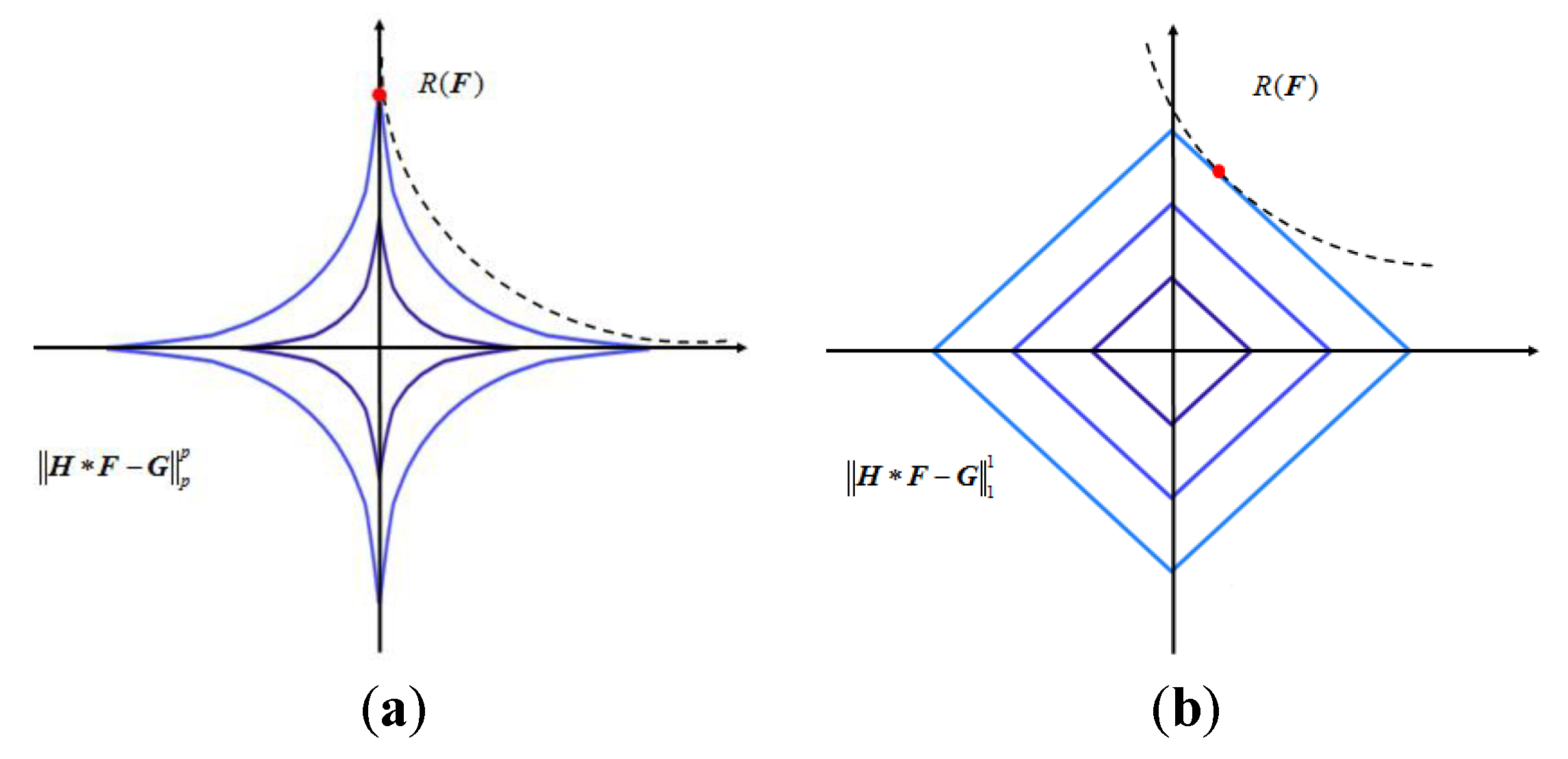
To better elaborate on this issue, the contours of the Lp-pseudo-norm are shown in Figure 1. Figure 2 presents a group of diagrams, where the contours represent the fidelity terms for image restoration, while the dashed lines represent the regularization terms. As shown in the figure, it is more likely for the regularization term to intersect with the fidelity term of p < 1 than that of p = 1 on the coordinate axis, thereby making the likelihood of obtaining a sparse solution greater. Therefore, by using the Lp-pseudo-norm as a constraint, it is possible to better extract the sparse characteristics of signals in the transform domain to more precisely restore the image in the optimization problem.

3. Model Proposal and Solution Method

3.1. Proposed Model

To use the FFT to achieve a faster algorithm computation speed, it is assumed that the image satisfies a periodic boundary condition. Moreover, the model is expressed as a matrix, and the gradient difference is expressed in the form of a convolution to avoid large-scale matrix multiplication operations, thereby facilitating the subsequent discussion. Combining the Lp-pseudo-norm with the TGV regularization, this study proposes a new regularization model for image restoration to more thoroughly extract the structural characteristics of the first-order and second-order gradient matrices of the image, and obtain a sparser solution. The model is named the TGV-Lp model, described below.
m i n F , V h , V v H F G p p + μ TGV 2 ( F ) = m i n F , V h , V v H F G p p + μ [ α 0 ( K h F V h 1 + K v F V v 1 ) + α 1 ( K h V h 1 + K v V v 1 + K v V h + K h V v 1 ) ] ,
where μ is the regularization parameter, p p represents the Lp-pseudo-norm, α 0 and α 1 serve as the balance coefficients, and V h , V v represent the horizontal and vertical gradients of the processed image.

3.2. Solution Method

To solve the model described by Equation (4), the complex optimization problem is decomposed into several sub-problems that are solved using the ADMM framework. Then, alternating iterations of the solutions of the sub-problems are performed until the solutions converge to the optimal solution of the original optimization problem. To this end, a series of intermediate variables X i are introduced, with X i N × N ( i = 0 5 ) , and they are defined as
{ X 0 = H F G X 1 = K h F V h X 2 = Κ v F V v X 3 = K h V h X 4 = K v V v X 5 = K v V h + Κ h V v .
The original problem is now transformed into the following constraint problem:
m i n F , V h , V v X 0 p p + μ [ α 0 ( X 1 1 + X 2 1 ) + α 1 ( X 3 1 + X 4 1 + X 5 1 ) ] s . t . X 0 = H F G , X 1 = K h F V h , X 2 = Κ v F V v , X 3 = K h V h , X 4 = K v V v , X 5 = K v V h + Κ h V v .
The augmented Lagrangian multiplier (ALM) method [20] is used to transform the constraint problem described by Equation (6) into an unconstrained augmented Lagrangian function as follows:
J = m a x Λ 0 ~ Λ 5 { m i n F , V h , V v , X 0 ~ X 5 X 0 p p + μ [ α 0 ( X 1 1 + X 2 1 ) + α 1 ( X 3 1 + X 4 1 + X 5 1 ) ] β 0 Λ 0 , X 0 ( H F G ) β 1 Λ 1 , X 1 ( K h F V h ) β 1 Λ 2 , X 2 ( K v F V v ) β 2 Λ 3 , X 3 K h V h β 2 Λ 4 , X 4 K v V v β 2 Λ 5 , X 5 ( K v V v + K h V v ) + β 0 2 ( X 0 ( H F G ) 2 2 + β 1 2 ( X 1 ( K h F V h ) 2 2 + X 2 ( K v F V v ) 2 2 ) + β 2 2 ( X 3 K h V h 2 2 + X 4 K v V v 2 2 + X 5 ( K v V h + K h V v ) 2 2 ) }
where μ 0 = μ α 0 and μ 1 = μ α 1 ; the dual variable Λ i N × N ( i = 0 5 ) is introduced as a Lagrangian multiplier, β j > 0   ( j = 0 2 ) is the penalty parameter, and X , Y represents the inner product of two matrices X and Y. Upon adding the term β j 2 ( Λ i 2 - Λ i 2 ) = 0   ( i = 0 5 , j = 0 2 ) to Equation (7) to complete the formula, Equation (8) is obtained after rearrangement.
J = m a x Λ 0 ~ Λ 5 { m i n F , V h , V v , X 0 ~ X 5 X 0 p p + μ [ α 0 ( X 1 1 + X 2 1 ) + α 1 ( X 3 1 + X 4 1 + X 5 1 ) ] + β 0 2 ( X 0 ( H F G ) Λ 0 2 2 + β 1 2 ( X 1 ( K h F V h ) Λ 1 2 2 + X 2 ( K v F V v ) Λ 2 2 2 ) + β 2 2 ( X 3 K h V h Λ 3 2 2 + X 4 K v V v Λ 4 2 2 + X 5 ( K v V h + K h V v ) Λ 5 2 2 ) β 0 2 Λ 0 2 β 1 2 ( Λ 1 2 + Λ 2 2 ) β 2 2 ( Λ 3 2 + Λ 4 2 + Λ 5 2 ) } , .

3.2.1. Solving Sub-Problems F, Vh, and Vv

According to the ADMM principle, F, Vh, and Vv are decoupled with the intermediate variables and the dual variables, while there is coupling between F, Vh, and Vv. It is necessary to establish Equation (9) to obtain a simultaneous solution.
{ J F = β 0 2 X 0 ( k ) ( H F G ) Λ 0 ( k ) 2 2 + β 1 2 [ X 1 ( k ) ( K h F V h ) Λ 1 ( k ) 2 2 + X 2 ( k ) ( K v F V v ) Λ 2 ( k ) 2 2 ] J V h = β 1 2 X 1 ( k ) ( K h F V h ) Λ 1 ( k ) 2 2 + β 2 2 [ X 3 ( k ) K h V h Λ 3 ( k ) 2 2 + X 5 ( k ) ( K v V h + K h V v ) Λ 5 ( k ) 2 2 ] J V v = β 1 2 X 2 ( k ) ( K v F V v ) Λ 2 ( k ) 2 2 + β 2 2 [ X 4 ( k ) K v V v Λ 4 ( k ) 2 2 + X 5 ( k ) ( K v V h + K h V v ) Λ 5 ( k ) 2 2 ) .
It is assumed here that the image to process satisfies a periodic boundary condition. According to the convolution law, the convolution result of two matrix spaces corresponds to the point multiplication of two matrix spectra in the frequency domain. To effectively avoid the computational complexity introduced by large-scale matrix operations, FFT is used for convolutional computation to solve the problem described by Equation (9). To this end, F, Vh, and Vv in Equation (9) are re-expressed in the frequency domain as follows:
{ J ¯ F = β 0 2 X ¯ 0 ( k ) ( H ¯ F ¯ G ¯ ) Λ ¯ 0 ( k ) 2 2 + β 1 2 [ X ¯ 1 ( k ) ( K ¯ h F ¯ V ¯ h ) Λ ¯ 1 ( k ) 2 2 + X ¯ 2 ( k ) ( K ¯ v F ¯ V ¯ v ) Λ ¯ 2 ( k ) 2 2 ] J ¯ V h = β 1 2 X ¯ 1 ( k ) ( K ¯ h F ¯ V ¯ h ) Λ ¯ 1 ( k ) 2 2 + β 2 2 [ X ¯ 3 ( k ) K ¯ h V ¯ h Λ ¯ 3 ( k ) 2 2 + X ¯ 5 ( k ) ( K ¯ v V ¯ h + K ¯ h V ¯ v ) Λ ¯ 5 ( k ) 2 2 ] J ¯ V v = β 1 2 X ¯ 2 ( k ) ( K ¯ v F ¯ V ¯ v ) Λ ¯ 2 ( k ) 2 2 + β 2 2 [ X ¯ 4 ( k ) K ¯ v V ¯ v Λ ¯ 4 ( k ) 2 2 + X ¯ 5 ( k ) ( K ¯ v V ¯ h + K ¯ h V ¯ v ) Λ ¯ 5 ( k ) 2 2 ) ,
where X ¯ denotes the frequency spectrum of X , and denotes the element-wise matrix multiplication operator. The right side of the equation is a smooth convex function. To seek the optimal solution of Equation (10), the partial differentiation of J ¯ F , J ¯ V h , J ¯ V v with respect to F ¯ , V ¯ h , V ¯ v is set to zero as follows:
{ J ¯ F F ¯ = β 0 ( H ¯ ) [ H ¯ F ¯ G ¯ ( X ¯ 0 ( k ) Λ ¯ 0 ( k ) ) ] + β 1 { K ¯ h [ K ¯ h F ¯ V ¯ h ( X ¯ 1 ( k ) Λ ¯ 1 ( k ) ) ] + K ¯ v [ K ¯ v F ¯ V ¯ v ( X ¯ 2 ( k ) Λ ¯ 2 ( k ) ) ] } = 0 J ¯ V h V ¯ h = β 1 [ K ¯ h F ¯ V ¯ h ( X ¯ 1 ( k ) Λ ¯ 1 ( k ) ) ] + β 2 { ( K ¯ h ) [ K ¯ h V ¯ h ( X ¯ 3 ( k ) Λ ¯ 3 ( k ) ) ] + ( K ¯ v ) [ K ¯ v V ¯ h + K ¯ h V ¯ v ( X ¯ 5 ( k ) Λ ¯ 5 ( k ) ) ] } = 0 J ¯ V v V ¯ v = β 1 [ ( K ¯ v F ¯ V ¯ v ( X ¯ 2 ( k ) Λ ¯ 2 ( k ) ) ] + β 2 { ( K ¯ v ) [ K ¯ v V ¯ v ( X ¯ 4 ( k ) Λ ¯ 4 ( k ) ) ] + ( K ¯ h ) [ K ¯ v V ¯ h + K ¯ h V ¯ v ( X ¯ 5 ( k ) Λ ¯ 5 ( k ) ) ] } = 0 .
For the sake of reading convenience, Equation (12) is re-formulated into simultaneous equations of the three variables F ¯ , V ¯ h , and V ¯ v .
{ A 11 F ¯ + A 12 V ¯ h + A 13 V ¯ v = B 1 A 21 F ¯ + A 22 V ¯ h + A 23 V ¯ v = B 2 A 31 F ¯ + A 32 V ¯ h + A 33 V ¯ v = B 3 .
By re-organizing Equation (11), we obtain
{ A 11 = β 0 ( H ¯ ) H ¯ +   β 1 ( K ¯ h ) K ¯ h + β 1 ( K ¯ v ) K ¯ v A 12 = β 1 ( K ¯ h ) A 13 = β 1 ( K ¯ v ) B 1 = β 0 ( H ¯ ) ( X ¯ 0 ( k ) + G ¯ Λ ¯ 0 ( k ) ) + β 1 ( K ¯ h ) ( X ¯ 1 ( k ) Λ ¯ 1 ( k ) ) + β 1 ( K ¯ v ) ( X ¯ 2 ( k ) Λ ¯ 2 ( k ) ) ,
{ A 21 = β 1 K ¯ h A 22 = β 1 1 + β 2 ( K ¯ h ) K ¯ h + β 2 ( K ¯ v ) K ¯ v A 23 = β 2   ( K ¯ v ) K ¯ h B 2 = β 1 ( Λ ¯ 1 ( k ) X ¯ 1 ( k ) ) + β 2 [ ( K ¯ h ) ( X ¯ 3 ( k ) Λ ¯ 3 ( k ) ) + ( K ¯ v ) ( X ¯ 5 ( k ) Λ ¯ 5 ( k ) ) ] ,
{ A 31 = β 1 K ¯ v A 32 = β 2 ( K ¯ h ) K ¯ v A 33 = β 1 1 + β 2 ( K ¯ h ) K ¯ h + β 2 ( K ¯ v ) K ¯ v B 3 = β 1 ( Λ ¯ 2 ( k ) X ¯ 2 ( k ) ) + β 2 [ ( K ¯ v ) ( X ¯ 4 ( k ) Λ ¯ 4 ( k ) ) + ( K ¯ h ) ( X ¯ 5 ( k ) Λ ¯ 5 ( k ) ) ] ,
where 1 denotes a matrix of ones. Now, F, Vh, and Vv can be solved using FFT based on Cramer’s rule.
{ F ( k + 1 ) = F 2 D 1 { | B 1 A 12 A 13 B 2 A 22 A 23 B 3 A 32 A 33 | / | A 11 A 12 A 13 A 21 A 22 A 23 A 31 A 32 A 33 | } V h ( k + 1 ) = F 2 D 1 { | A 11 B 1 A 13 A 21 B 2 A 23 A 31 B 3 A 33 | / | A 11 A 12 A 13 A 21 A 22 A 23 A 31 A 32 A 33 | } V v ( k + 1 ) = F 2 D 1 { | A 11 A 12 B 1 A 21 A 22 B 2 A 31 A 32 B 3 | / | A 11 A 12 A 13 A 21 A 22 A 23 A 31 A 32 A 33 | } .
In Equation (16), F 2 D 1 denotes a two-dimensional inverse Fourier transform, and the division symbol / denotes element-wise matrix division. According to Cramer’s rule, | | in Equation (16) refers to the following: | Y 11 Y 12 Y 13 Y 21 Y 22 Y 23 Y 31 Y 32 Y 33 | = Y 11 Y 22 Y 33 + Y 12 Y 23 Y 31 + Y 13 Y 21 Y 32   Y 13 Y 22 Y 31 Y 12 Y 21 Y 33   Y 11 Y 32 Y 23 .

3.2.2. Solving Sub-Problems Containing Intermediate Variables X i ( i = 0 , 1 , 2 , , 5 )

For the sub-problems containing intermediate variables of X i ( i = 0 , 1 , 2 , , 5 ) , the objective functions are expressed as
{ J X 0 = m i n X 0 X 0 p p + β 0 2 ( X 0 ( H F ( k + 1 ) G ) Λ 0 ( k ) 2 2 J X 1 = m i n X 1 μ 0 X 1 1 + β 1 2 X 1 ( K h F ( k + 1 ) V h ( k + 1 ) ) Λ 1 ( k ) 2 2 J X 2 = m i n X 2 μ 0 X 2 1 + β 1 2 X 2 ( K v F ( k + 1 ) V v ( k + 1 ) ) Λ 2 ( k ) 2 2 J X 3 = m i n X 3 μ 1 X 3 1 + β 2 2 X 3 K h V h ( k + 1 ) Λ 3 ( k ) 2 2 J X 4 = m i n X 4 μ 1 X 4 1 + β 2 2 X 4 K v V v ( k + 1 ) Λ 4 ( k ) 2 2 J X 5 = m i n X 5 μ 1 X 5 1 + β 2 2 X 5 ( K v V h ( k + 1 ) + K h V v ( k + 1 ) ) Λ 5 ( k ) 2 2 .
To solve the sub-problem of X 0 in Equation (17), Lp shrinkage [16,17] is used, with the Lp shrinkage operator defined as s h r i n k p ( ξ , τ ) = sgn ( ξ ) m a x { | ξ | τ 2 p | ξ | p 1 , 0 } . In the case of p = 1, the Lp shrinkage operator degenerates into a soft-threshold shrinkage operator. Soft-threshold shrinkage of the sub-problems of X 1 ~ X 5 gives
{ X 0 ( k + 1 ) = s h r i n k p ( H F ( k + 1 ) G + Λ 0 ( k ) , 1 β 0 ) X 1 ( k + 1 ) = s h r i n k ( K h F ( k + 1 ) V h ( k + 1 ) + Λ 1 ( k ) , μ 0 β 1 ) X 2 ( k + 1 ) = s h r i n k ( K v F ( k + 1 ) V v ( k + 1 ) + Λ 2 ( k ) , μ 0 β 1 ) X 3 ( k + 1 ) = s h r i n k ( K h V h ( k + 1 ) + Λ 3 ( k ) , μ 1 β 2 ) X 4 ( k + 1 ) = s h r i n k ( K v V v ( k + 1 ) + Λ 4 ( k ) , μ 1 β 2 ) X 5 ( k + 1 ) = s h r i n k ( K v V h ( k + 1 ) + K h V v ( k + 1 ) + Λ 5 ( k ) , μ 1 β 2 ) .

3.2.3. Solving Sub-Problems Containing Dual Variables Λ i ( i = 0 , 1 , 2 , , 5 )

For the sub-problems containing dual variables Λ i ( i = 0 , 1 , 2 , , 5 ) , the objective functions are expressed as
{ J Λ 0 = m a x Λ 0 β 0 Λ 0 , ( H F ( k + 1 ) G ) X 0 ( k + 1 ) J Λ 1 = m a x Λ 1 β 1 Λ 1 , ( K h F ( k + 1 ) V h ( k + 1 ) ) X 1 ( k + 1 ) J Λ 2 = m a x Λ 2 β 1 Λ 2 , ( K v F ( k + 1 ) V v ( k + 1 ) ) X 2 ( k + 1 ) J Λ 3 = m a x Λ 3 β 2 Λ 3 , ( K h V h ( k + 1 ) ) X 3 ( k + 1 ) J Λ 4 = m a x Λ 4 β 2 Λ 4 , ( K v V v ( k + 1 ) ) X 4 ( k + 1 ) J Λ 5 = m a x Λ 5 β 2 Λ 5 , ( K v V h ( k + 1 ) + K h V v ( k + 1 ) ) X 5 ( k + 1 ) .
In the ADMM framework, dual variables can be updated using the ascending gradient method as follows:
{ Λ 0 ( k + 1 ) = Λ 1 ( k ) + γ β 0 ( H F ( k + 1 ) G X 0 ( k + 1 ) ) Λ 1 ( k + 1 ) = Λ 1 ( k ) + γ β 1 ( K h F ( k + 1 ) V h ( k + 1 ) X 1 ( k + 1 ) ) Λ 2 ( k + 1 ) = Λ 2 ( k ) + γ β 1 ( K v F ( k + 1 ) V v ( k + 1 ) X 2 ( k + 1 ) ) Λ 3 ( k + 1 ) = Λ 3 ( k ) + γ β 2 ( K h V h ( k + 1 ) X 3 ( k + 1 ) ) Λ 4 ( k + 1 ) = Λ 4 ( k ) + γ β 2 ( K v V v ( k + 1 ) X 4 ( k + 1 ) ) Λ 5 ( k + 1 ) = Λ 5 ( k ) + γ β 2 ( K v V h ( k + 1 ) + K h V v ( k + 1 ) X 5 ( k + 1 ) ) ,
where γ denotes the learning rate or the slack variable. The convergence of the algorithm was proven in the case of γ ( 0 , 5 + 1 2 ) [21]. Hitherto, all the sub-problems of the model proposed in this study were solved, and the algorithm is herein referred to as TGV_Lp, which is summarized in Algorithm 1.
Algorithm 1. Pseudocode TGV_Lp for image restoration
Input: G , H
Output: F
Initialize:
k = 1 , X i ( k ) = 0 , Λ i ( k ) = 0 , ( i = 0 , 1 , , 5 ) , F ( k ) = 0 , μ 0 , μ 1 , β i ( i = 0 , 1 , 2 ) , γ , p , t o l .
1: Set F ( k + 1 ) F ( k ) 2 / F ( k ) 2 as 1;
2: While F ( k + 1 ) F ( k ) 2 / F ( k ) 2 > t o l do
3:   Update F ( k + 1 ) , V h ( k + 1 ) , V v ( k + 1 ) according to Equation (16);
4:   Update X i ( k + 1 ) ( i = 0 , 1 , , 5 ) according to Equation (18);
5:   Update Λ i ( k + 1 ) ( i = 0 , 1 , , 5 ) according to Equation (20);
6:   k = k + 1;
7: End while
8: Return F ( k ) as F .

4. Numerical Experiments

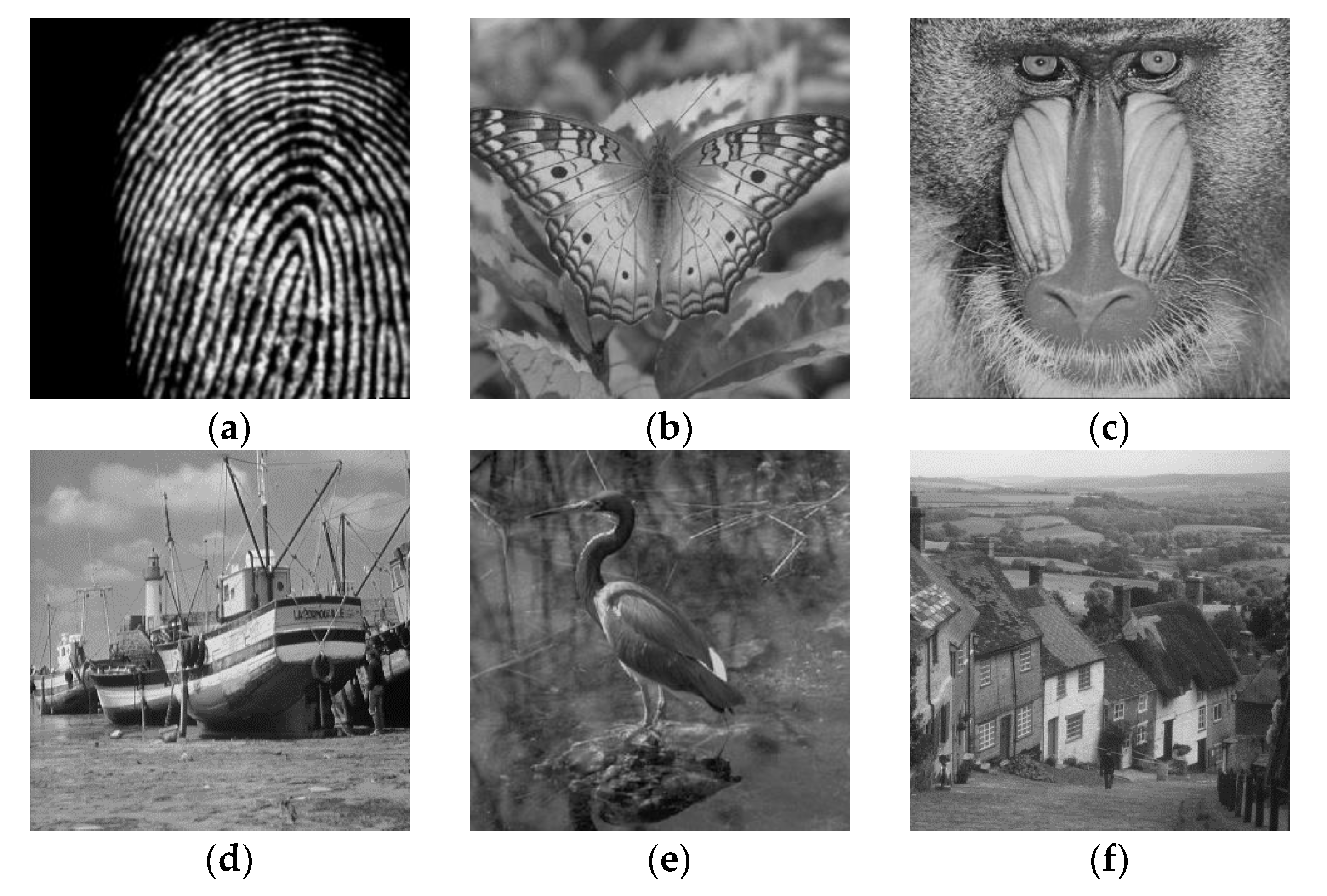
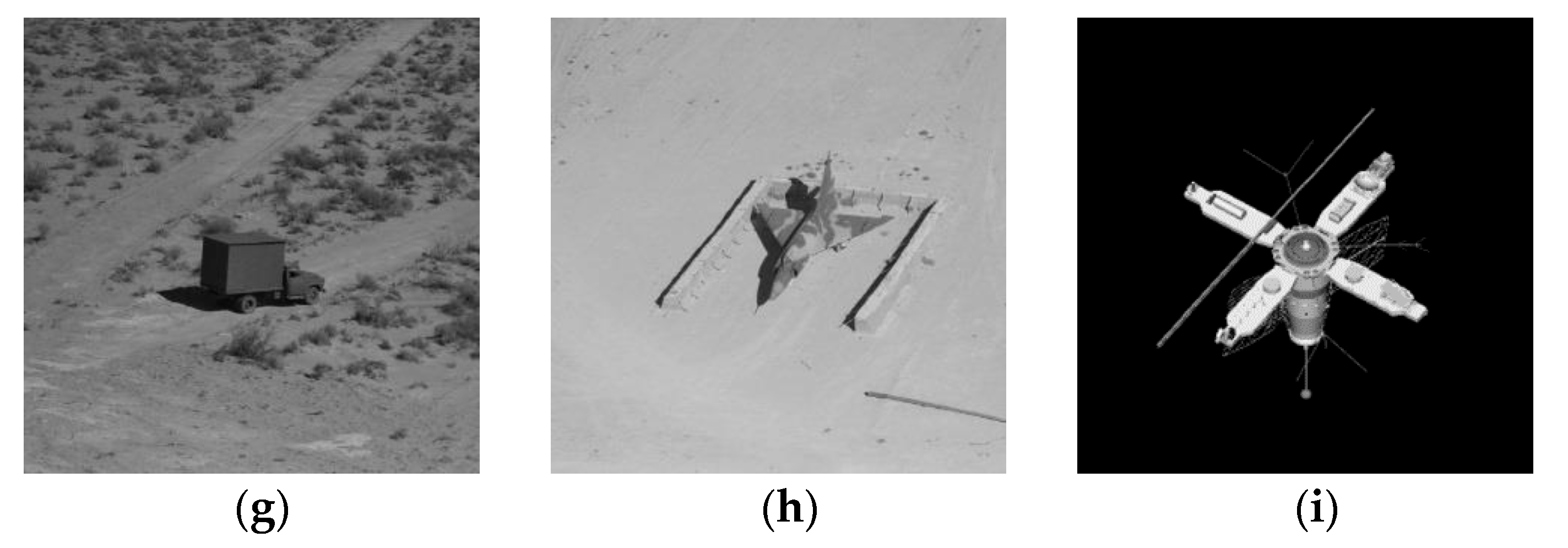
To verify the appropriateness and validity of the proposed model, standard images of different styles were selected as experimental objects. The images were degraded with Gaussian blur, average blur, motion blur, and different degrees of impulse noise so that a large number of numerical simulation experiments could be performed to make indicator-based comparisons and evaluations in an objective manner. In particular, the image “Satellite” was downloaded from the Emory University image database [27], and the other images were downloaded from CVG-UGR (Computer Vision Group, University of Granada) image database [28]. These test images were widely used in other relevant publications, thereby allowing for objective and fair comparison of the test results. All calculations in this study were performed using MATLAB R2018a on a Windows 10 system with an Intel ® Core ™ i7-7700 central processing unit (CPU) (4.2 GHz) with 16.0 GB of memory.

4.1. Evaluation Indicators and Stopping Criteria

For objective evaluation of image quality, PSNR, SSIM, and SNR were used. Their definitions are given below [29].
P S N R ( X , Y ) = 10 l o g 10 L 2 1 N 2 i = 1 N j = 1 N ( X i j Y i j ) 2 ,
where X represents an original image, and Y represents a restored image; L represents the maximum gray level of the image, which was set as 255 in this study. Generally, a larger PSNR value of a restored image denotes less image distortion and greater similarity between the restored image and the original image.
S S I M ( X , Y ) = ( 2 μ X μ Y + L 2 k 1 2 ) ( 2 σ X Y + L 2 k 2 2 ) ( μ X 2 + μ Y 2 + L 2 k 1 2 ) ( σ X 2 + σ Y 2 + L 2 k 2 2 ) ,
where μ X and μ Y represent the means of images X and Y, respectively, σ X 2 and σ Y 2 represent the variances of X and Y, respectively, σ X Y represents the covariance of X and Y, and the constants k 1 and k 2 are very small positive numbers introduced to prevent the denominator of Equation (22) from being zero; they were set as 0.01 and 0.03 in this study, respectively. The maximum value of SSIM is 1, which indicates that the original image and the restored image are 100% identical; as the value of SSIM approaches 1, the similarity between the original and restored images increases.
S N R ( X , Y ) = 10 l o g 10 X 2 2 X Y 2 2 .
Images with low noise have higher SNR values, making SNR an important metric for characterizing the performance of the restoration algorithm.
In the experiments, the iteration stopping criterion for comparing various algorithms was Equation (24), where F ( k ) and F ( k + 1 ) denote the objective functions after the k-th iteration and (k + 1)-th iteration, respectively.
F ( k + 1 ) F ( k ) 2 F ( k ) 2 1 < 10 4 .
The blur kernels used in the test were Gaussian blur, average blur, and motion blur, all of which were generated by built-in functions of MATLAB. The function fspecial (‘gaussian’, S , σ ) generates an S × S Gaussian blur kernel standard deviation of σ , and the kernel is hereinafter referred to as ( G , S , σ ) for convenience; fspecial (‘average’, S ) generates an S × S average blur kernel, which is referred to as ( A , S ) ; fspecial (‘motion’, L , θ ) generates a motion blur kernel with a length of L and angle of θ , which is referred to as ( M , L , θ ) . Noise effects were generated by built-in function imnoise (Ib, ‘salt & pepper’, level), where “Ib” is the blurred image and “level” is the noise density, i.e., the percentage of noise in the total number of pixels.

4.2. Parameter Selection and Sensitivity Analysis

Parameters involved in the algorithm of this study are μ 0 ,   μ 1 ,   β i ( i = 0 , 1 , 2 ) , p ,   and   γ . In particular, μ 0 = μ α 0 and μ 1 = μ α 1 are regularization parameters with values greater than zero, which serve to balance the fidelity term and regularization term. Based on our previous experience with testing, we assumed here that α 0 = 2 α 1 while gradually increasing the value of μ between 0.1 and 10 to find the optimal effect of image restoration. Given the characteristics of impulse noise, the value of the Lp-pseudo-norm was gradually increased from 0.1 to 1 by a step of 0.05, and a loop statement was adopted to traverse all paths to find the p value for the optimal PSNR. In all tests, the penalty parameter β i ( i = 0 , 1 , 2 ) of the ALM method was set to have ratios of β 0 : β 1 : β 2 = 50 : 1 : 5 , and the slack variable was set to 1, i.e., γ = 1 .

4.2.1. Regularization Parameter μ

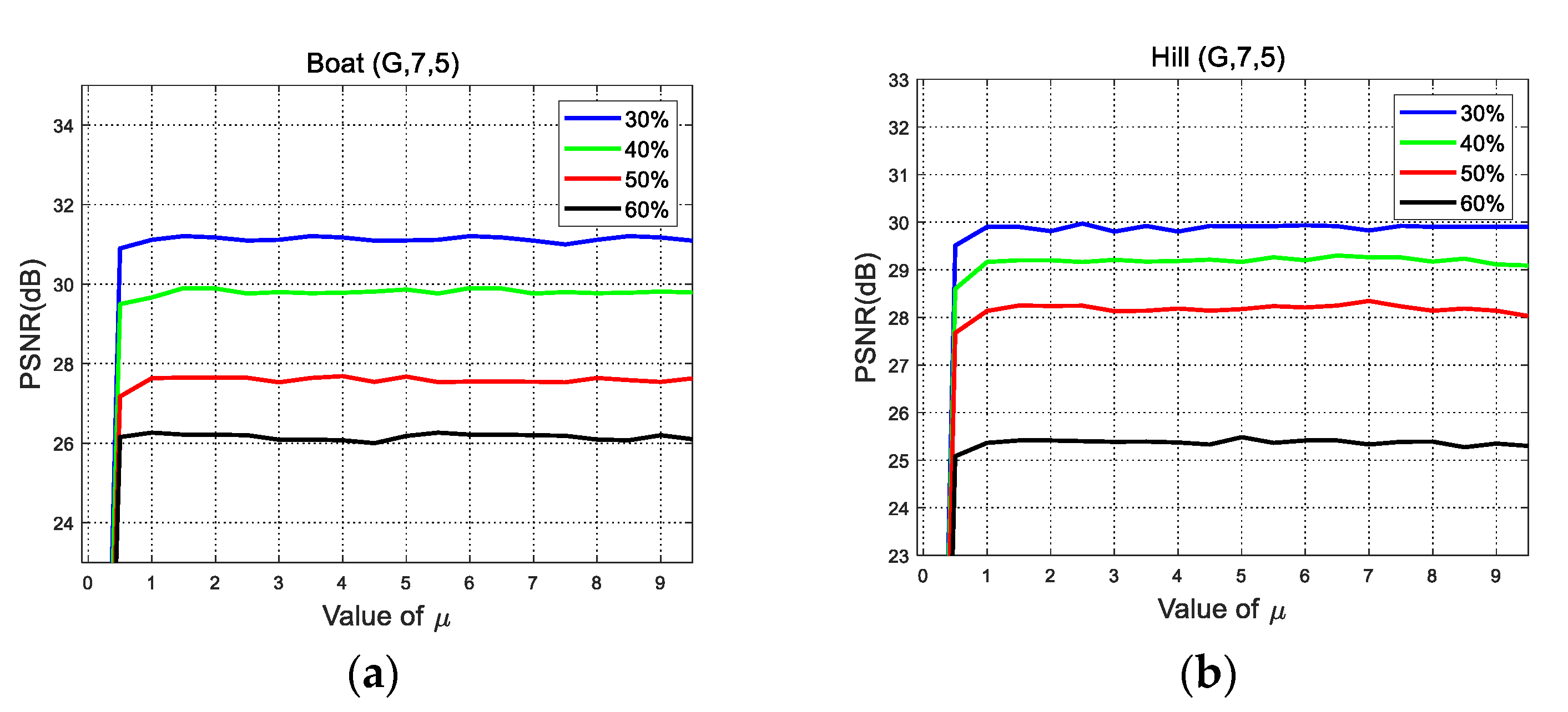
To test the effect of the regularization parameter μ on the image restoration results, different levels of blur and impulse noise were introduced into the test images (a)–(i), and PSNR values were recorded by gradually increasing the value of μ in the range of 0.1–10 while fixing other parameters. The experimental results show that the proposed algorithm is not sensitive to μ ; that is, during the recovery process of different images, the value of PSNR does not undergo significant changes with changes in μ , indicating that the proposed algorithm is robust. The test results of the “Boat” image of Figure 3d and “Hill” image of Figure 3f treated with the Gaussian blur kernel at 30%, 40%, 50%, and 60% noise levels are presented in Figure 4. The PSNR value in Figure 4 was not optimal for the proposed algorithm, as other fixed parameters remained to be adjusted optimally. In subsequent experiments, the regularization parameter was set to 1, i.e., μ = 1 .

4.2.2. Value of p in Lp-Pseudo-Norm

When it came to selecting the p value of the Lp-pseudo-norm, given the characteristics of the impulse noise, the p value was gradually increased from 0.1 to 1 in steps of 0.05, and a loop statement was adopted to traverse all paths so as to find the p value that could give the optimal PSNR value of image restoration. For restoration of the nine images treated with ( G , 7 , 5 ) at 30–60% noise levels, the best p values were obtained and are listed in Table 1, with the results showing that the p value was relatively stable for the same image.
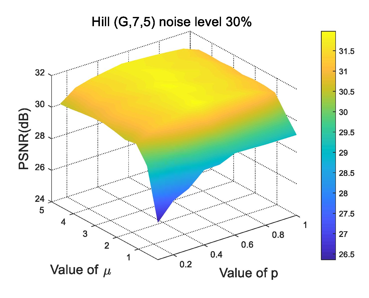
In addition, to better show the best selection of the p and μ values, we used a three-dimensional (3D) figure. The test results of the “Hill” image treated with the Gaussian blur kernel at 30% noise level are presented in Figure 5.

4.3. Numerical Performance Comparison

To test the effectiveness of the proposed algorithm, the following four algorithms were compared: an FTVd model, a TGV model, an OGSTV model, and the proposed frequency-domain TGV-Lp model. The algorithms were adapted from the authors’ web pages or shared by the authors. It is noteworthy that all these algorithms are state-of-the-art algorithms in the field of image restoration. In the experiments, regularization parameters were adjusted until each algorithm achieved its best performance for image restoration to ensure an objective and fair comparison.

4.3.1. Numerical Performance Comparison for Image Recovery in the Presence of Gaussian Blur

The results of the image restoration tests performed on nine test images degraded with Gaussian blur kernel ( G , 7 , 5 ) and 30–60% impulse noise are listed in Table 2. In the table, the optimal indicators are highlighted in bold.
The results of image restoration tests performed on nine test images degraded with a Gaussian blur kernel ( G , 15 , 5 ) and 30% noise are shown in Table 3.
An in-depth analysis of the data in Table 2 and Table 3 leads to the following conclusions:
  • All four methods can effectively recover images that were degraded by Gaussian blur and different degrees of impulse noise. The PSNR, SSIM, and SNR values of the proposed method are generally higher than those of other competitive methods, which indicates that the proposed method has better deblurring and denoising effects. In particular, for images with many lines and complex textures, such as “Fingerprint” in Figure 3a, “Butterfly” in Figure 3b, and “Baboon” in Figure 3c, the proposed method performed well, especially at high noise levels. For example, for the “Fingerprint” image of Figure 3a treated with a Gaussian blur kernel ( G , 7 , 5 ) and 50% noise, the PSNR value (35.59 dB) of the proposed method was higher by 7.22 dB than that of the FTVd method (28.37 dB), and was higher by 2.55 dB and 1.6 dB than that of the TGV method (33.04 dB) and the OGSTV method (33.99 dB), respectively.
  • When restoring the nine degraded images treated with the Gaussian blur kernel ( G , 7 , 5 ) and 30–60% impulse noise, the proposed method achieved 0.58–2.85 dB higher PSNR values compared with the TGV method. When restoring the nine degraded images treated with the Gaussian blur kernel ( G , 15 , 5 ) and impulse noise, the proposed method achieved 0.45–1.73 dB higher PSNR values compared with the TGV method. For example, for the “Bird” image of Figure 3e treated with the Gaussian blur kernel ( G , 7 , 5 ) and two different levels (50% vs. 60%) of noise, the PSNR values of the proposed method (32.31 dB and 29.69 dB) were 2.85 dB and 2.7 dB higher than those of the TGV method (29.46 dB and 26.99 dB), respectively.
  • The OGSTV method is an excellent algorithm for image deblurring and impulse noise removal, and it uses the neighborhood gradient information of the image to form a combined gradient for image restoration, which achieves good image restoration performance for smooth image regions but is less satisfactory in recovering image edge regions containing sharp lines and angles. In the test, it was observed that, for smooth images with non-complex textures, such as the “Plane” image of Figure 3h and “Satellite” image of Figure 3i, the OGSTV method had particularly excellent performance, which was slightly better than that of the proposed algorithm in the case of low noise levels. In the case of high noise levels, however, the proposed algorithm was still superior to the OGSTV method. For example, when restoring the “Satellite” image degraded with ( G , 7 , 5 ) and 30% noise, the OGSTV method achieved a slightly higher PSNR value of 36.97 dB compared to the proposed method (36.54 dB), with a difference of only 0.43 dB; however, in the cases of 50% and 60% noise, the PSNR values of the OGSTV method were lower than those of the proposed method.
The above analysis indicates that the use of Lp-pseudo-norm shrinkage in the proposed method increases the degree of freedom by one, making it less difficult to describe image gradient sparsity. The performance of the proposed method in removing Gaussian blur and impulse noise is generally better than that of the three competitive methods, especially for images with complex textures. In addition, the comparison reveals that the image restoration performance of the FTVd algorithm is much worse than that of the other three algorithms; thus, the subsequent experimental results of the FTVd algorithm are not listed in some tables.

4.3.2. Numerical Performance Comparison for Image Recovery in the Presence of Average Blur

The image restoration capability of the proposed method for degraded images treated with average blur and impulse noise was investigated, with Table 4 presenting the results of image restoration tests performed on nine degraded test images treated with an average blur kernel ( A , 7 ) and two levels (30% vs. 60%) of noise.
With regard to the image restoration performance of the algorithms for different images treated with average blur and different levels of impulse noise, the data in Table 4 lead to conclusions similar to those obtained in the case of Gaussian blur and impulse noise. When restoring the nine degraded test images treated with an average blur kernel ( A , 7 ) and impulse noise, the proposed method achieved 0.48–4.16 dB higher PSNR values compared with the TGV method. For images with many lines and complex textures, such as the “Fingerprint” image of Figure 3a, “Butterfly” image of Figure 3b, and “Baboon” image of Figure 3c, the proposed method achieved 0.8–2.14 dB higher PSNR values compared with the OGSTV method. However, the OGSTV performed well in restoring smooth images in the presence of low noise levels.

4.3.3. Numerical Performance Comparison for Image Recovery in the Presence of Motion Blur

Furthermore, the image restoration capability of the proposed method in the case of motion blur and impulse noise was investigated. Table 5 presents the PSNR results of image restoration tests performed on the degraded “Butterfly” image of Figure 3b, “Baboon” image of Figure 3c, “Bird” image of Figure 3e, and “Truck” image of Figure 3g treated with different motion blur kernels and 30–60% noise.
For different images treated with varying degrees of motion blur and impulse noise, the data in Table 5 reveal that the proposed method outperformed the TGV and OGSTV methods in removing motion blur and impulse noise. When restoring the four images, the proposed method achieved 0.52–5.50 dB and 0.21–2.83 dB higher PSNR values than the TGV method and the OGSTV method, respectively.

4.4. Comparison of Visual Effects

To better observe the test results, some restored images are presented below for visual comparison purposes.

4.4.1. Comparison of the Visual Effects of Restored Images in the Case of Gaussian Blur

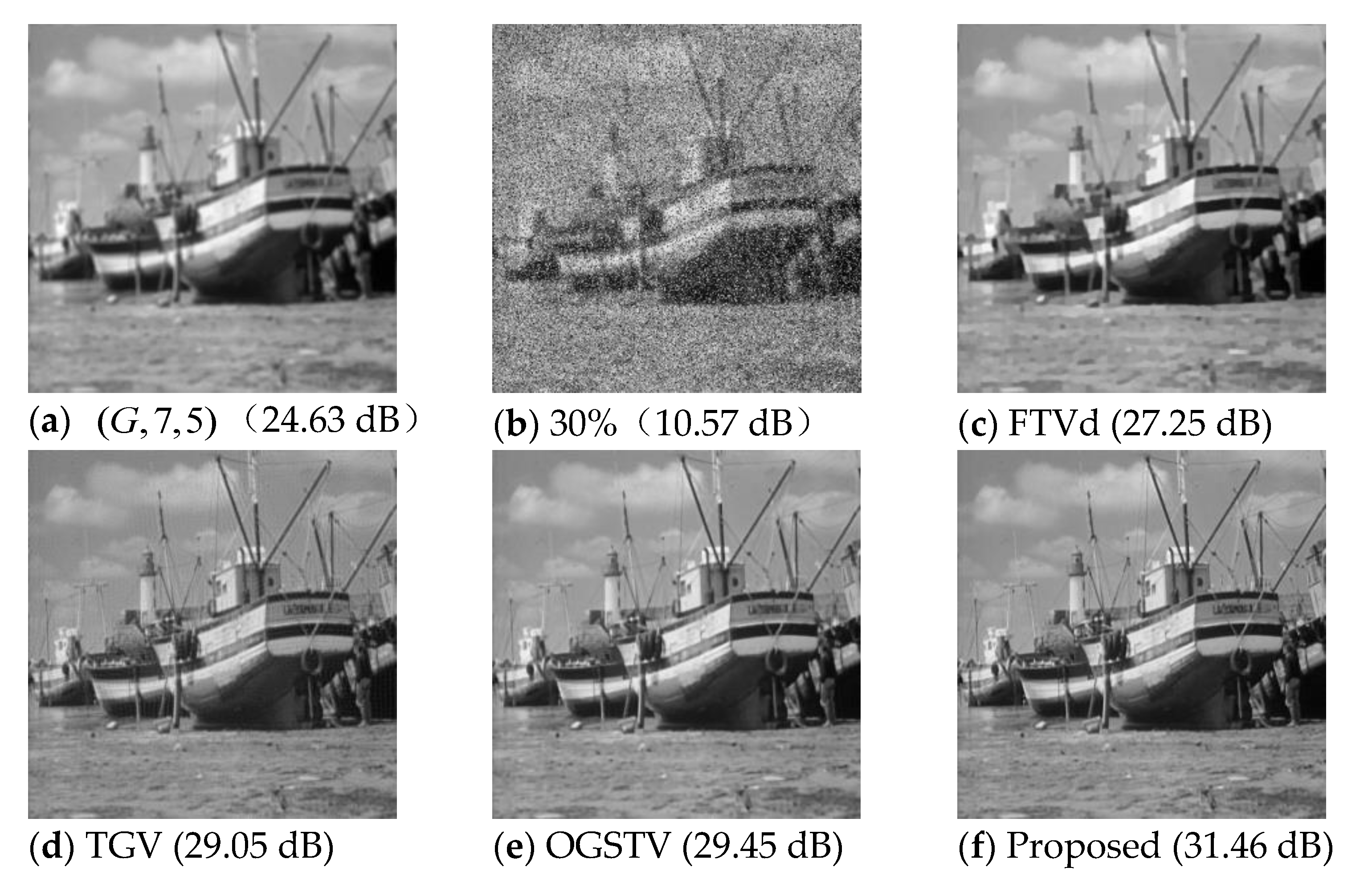
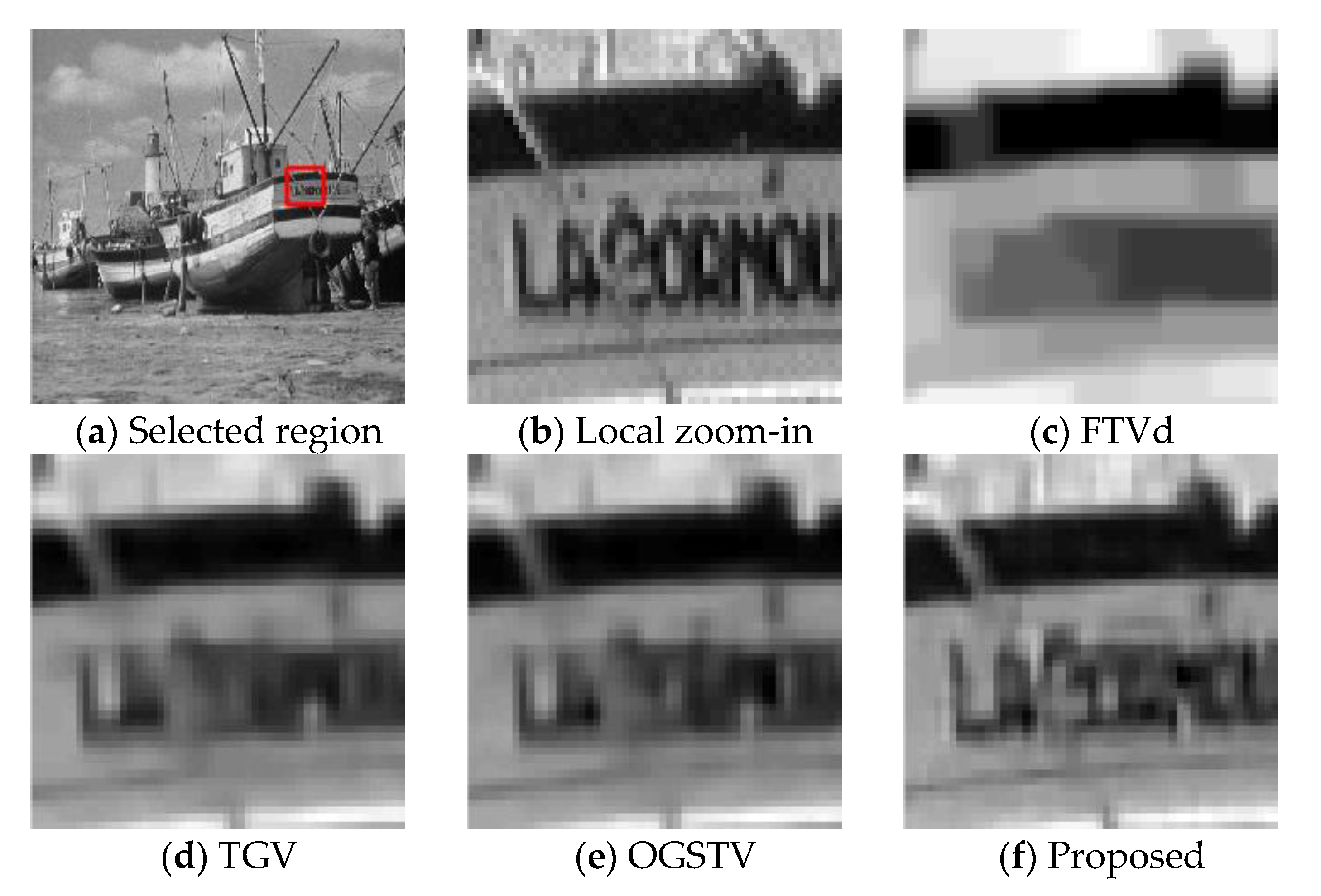
Figure 6 and Figure 7 present image restorations by the four algorithms of the “Boat” image degraded with a Gaussian blur kernel ( G , 7 , 5 ) and 30% impulse noise, and zoomed-in images of the restored images for better comparison, respectively. With respect to the visual effects of the restored images, with the FTVd method (c), a loss of some image details occurred during restoration of the image, and there was an obvious staircase effect. The TGV method (d) and the OGSTV method (e) performed well in suppressing the staircase effect, but slight ringing artefacts were generated when the TGV method was used to restore the image. Furthermore, the OGSTV method performed well in smooth image regions but relatively poorly preserved image edges. The proposed method, however, not only preserved image edges, but also restored smooth image regions well, achieving the best overall visual effects for image restoration.

4.4.2. Visual Effect Comparison for Image Restoration in the Case of Average Blur

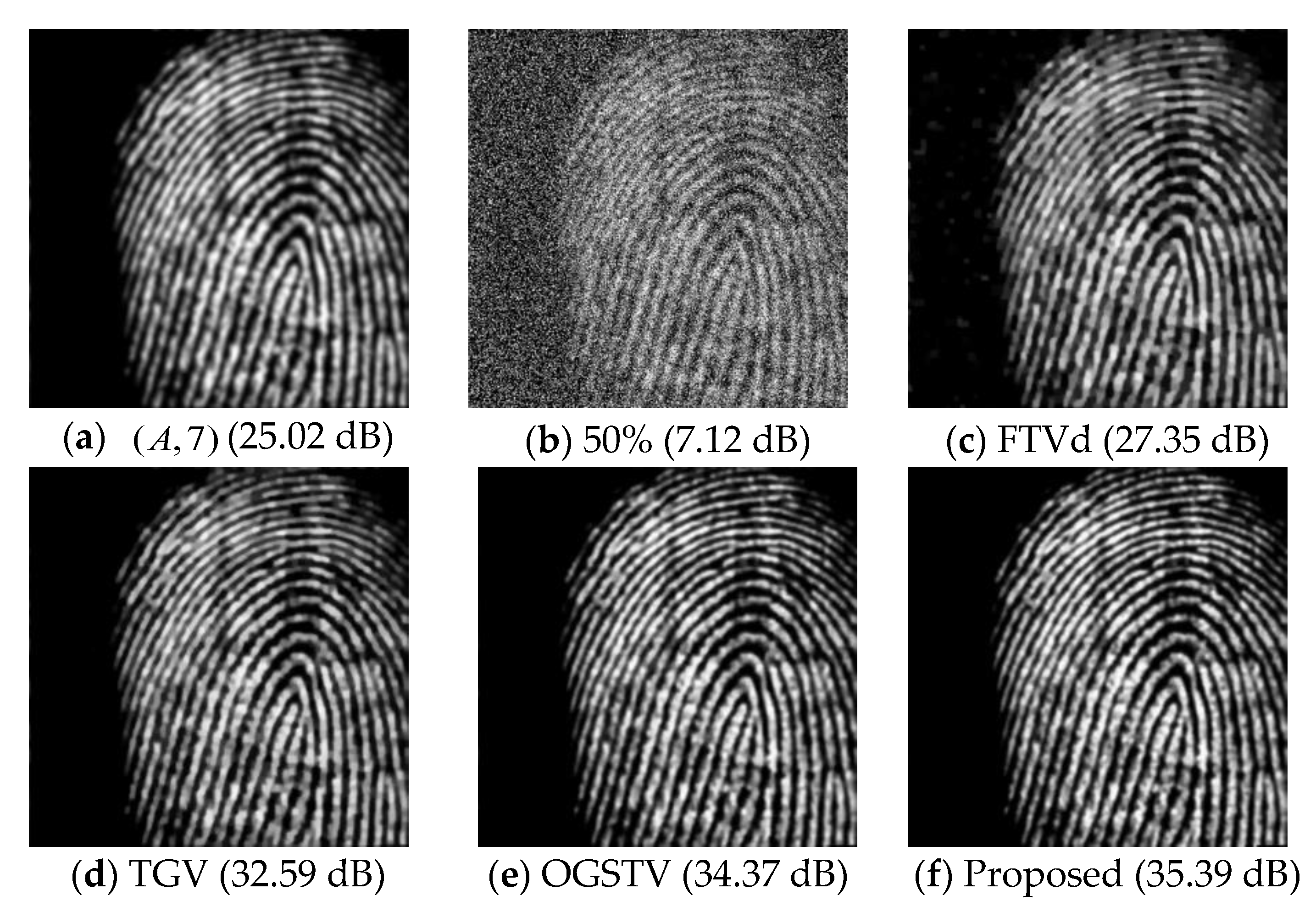
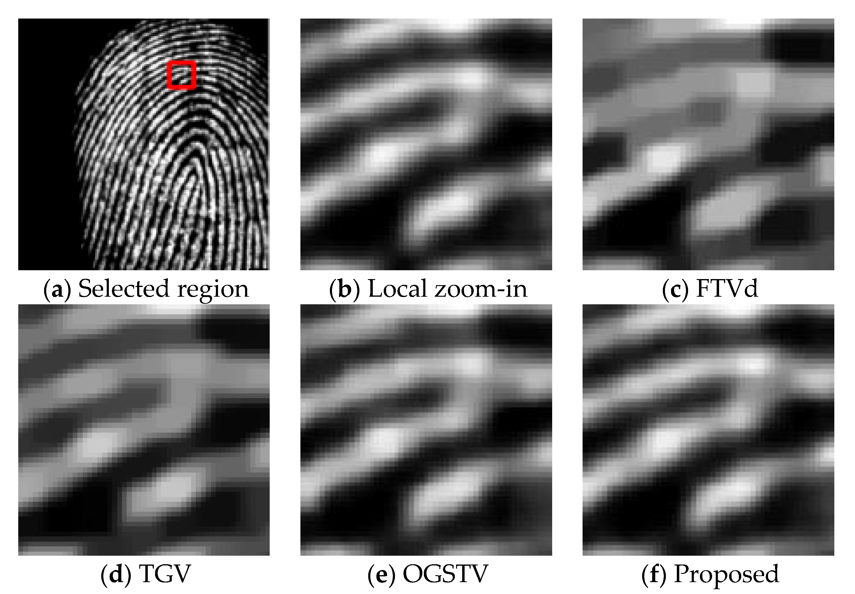
Figure 8 and Figure 9 present the “Fingerprint” image restored using the four algorithms from the image degraded with average blur kernel ( A , 7 ) and 50% impulse noise, as well as the zoomed-in restored images for better comparison. With respect to the visual effects of the restored images, the FTVd method (c) led to a certain degree of staircase effect in the restored image, the TGV method (d) led to blurred image edges in the restored image, and the OGSTV method (e) needed to be improved in preserving image edges. In contrast, the proposed method performed well in restoring the details of the image lines.

4.4.3. Visual Effect Comparison for Image Restoration of Images Degraded with Motion Blur

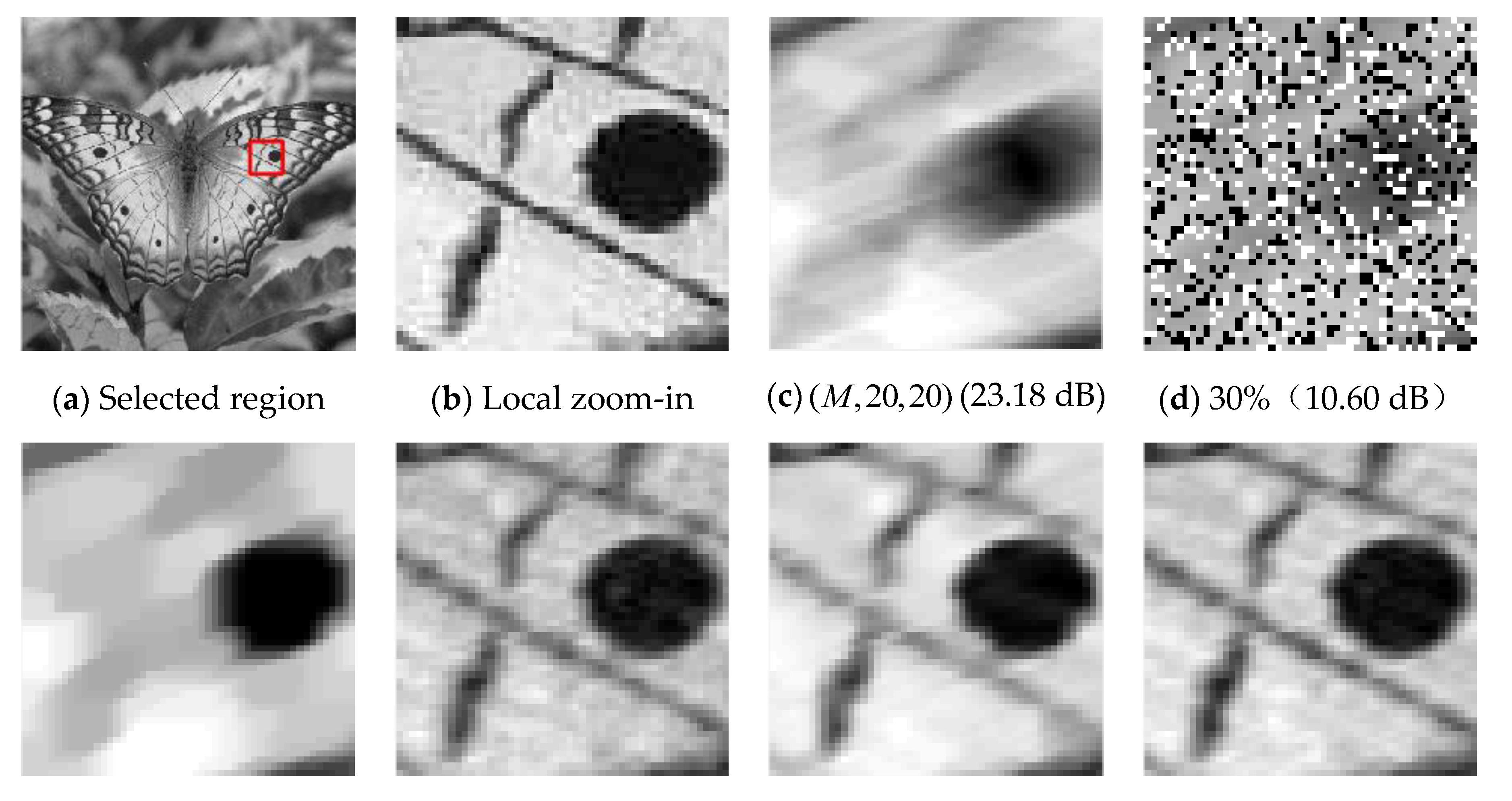
Figure 10 compares the zoomed-in details of the “Butterfly” image restored using the four algorithms with those of the image degraded with a motion blur kernel ( M , 20 , 20 ) and 30% impulse noise.
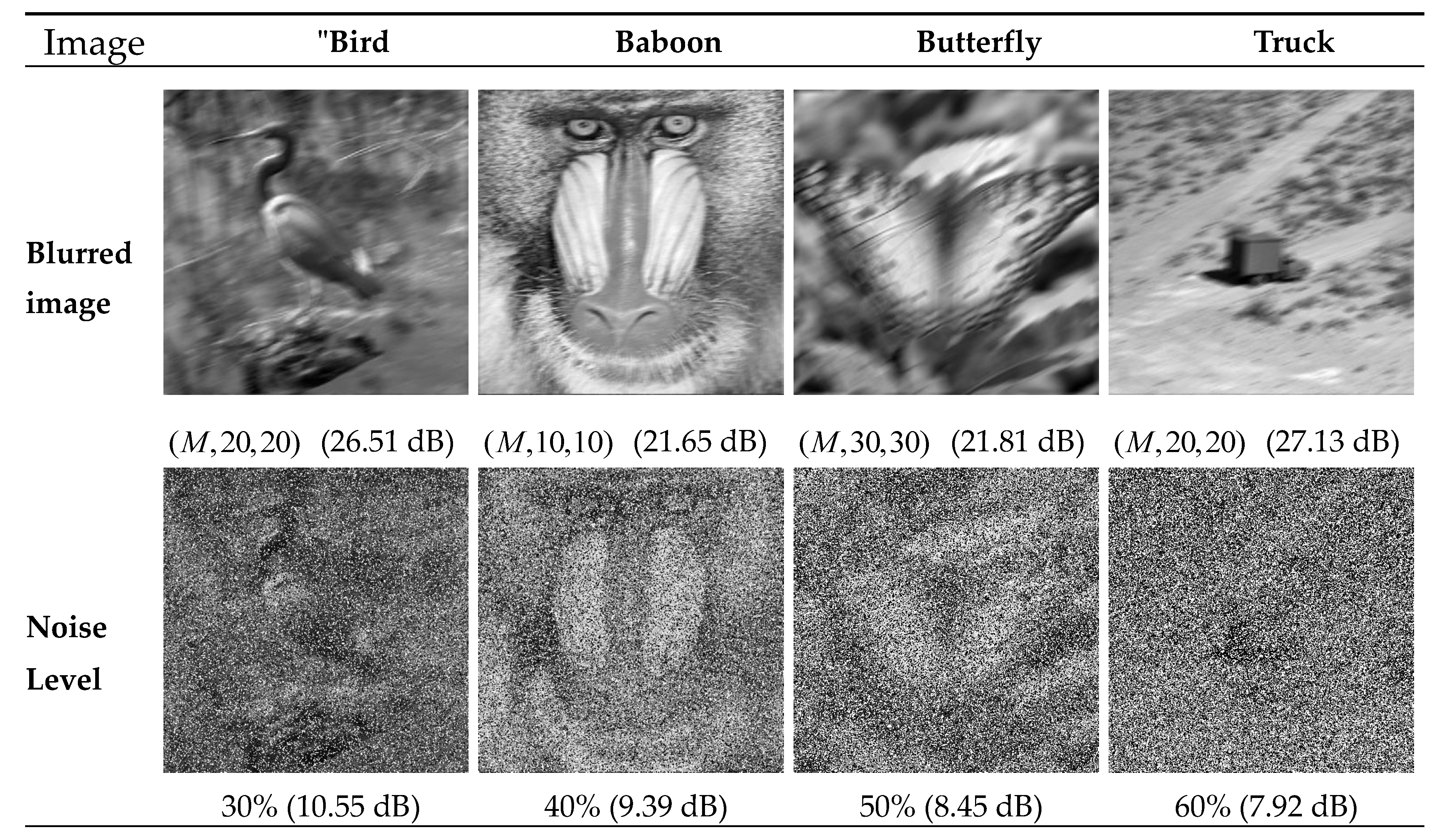
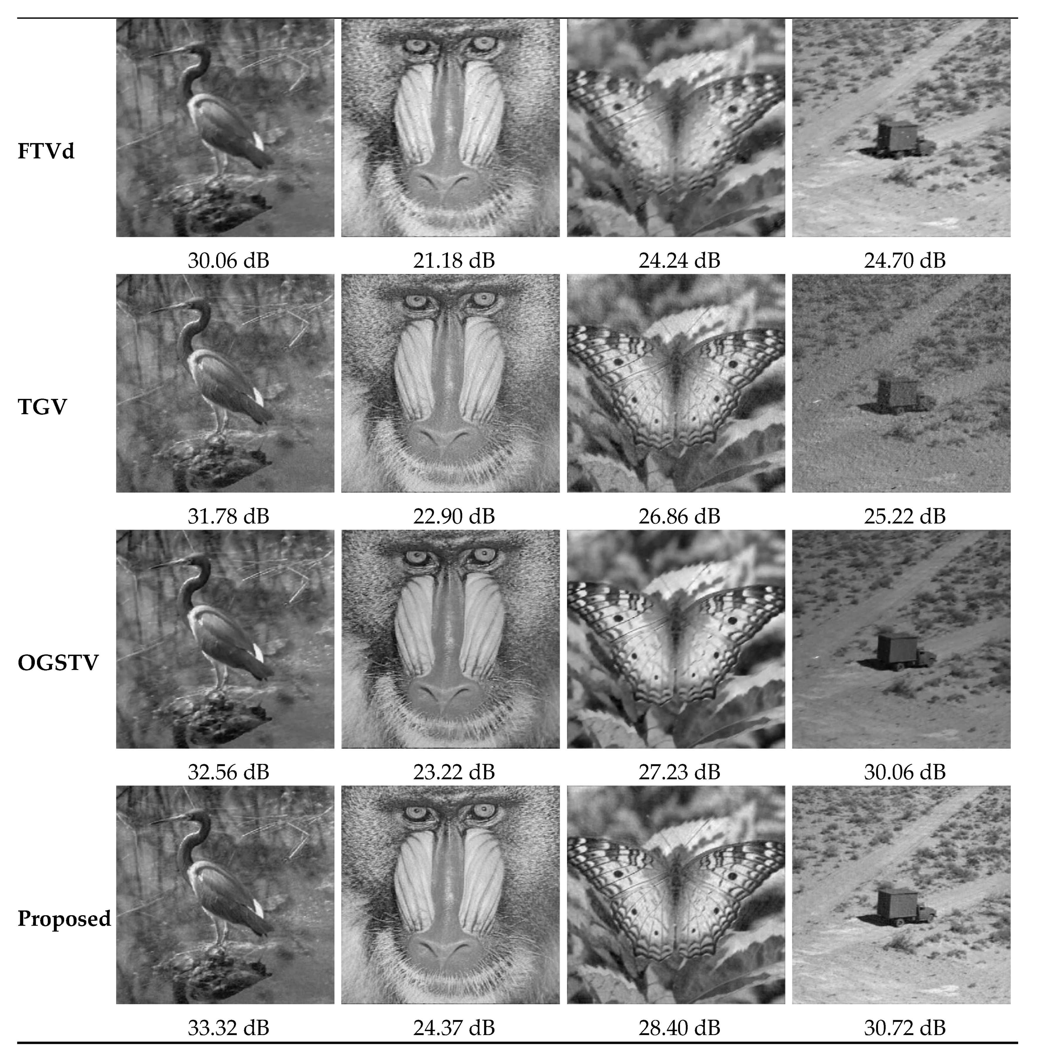
Figure 11 presents a visual effects comparison of the image restorations using the four algorithms for the following images: the “Bird” image degraded with a motion blur kernel ( M , 20 , 20 ) and 30% noise, the “Baboon” image degraded with a motion blur kernel ( M , 10 , 10 ) and 40% noise, the “Butterfly” image degraded with a motion blur kernel ( M , 30 , 30 ) and 50% noise, and the “Truck” image degraded with a motion blur kernel ( M , 20 , 20 ) and 60% noise. As shown in the figure, the proposed method allowed for better preservation of the smooth image regions and restoration of the details of the image lines with fewer artefacts.

4.5. Comparison of Computing Time

Finally, to further test the timeliness of the proposed model, the proposed method was compared with the FTVd, TGV, and OGSTV methods by testing the mean time required to restore the nine images of Figure 3 for different blur kernels at various impulse noise levels. Some test results are shown in Table 6, where the best indicators are highlighted in bold.
The calculation times in the table reveal that FTVd, which is a classic algorithm, is still advantageous in terms of computing speed. The proposed method is comparable to the OGSTV method in terms of image restoration time, while they are both faster than the TGV method. The proposed method uses the Lp-pseudo-norm as a regularization constraint, which increases the method’s computational burden, thereby leading to a certain degree of increase in the image restoration time. However, the gradient difference is re-expressed in the form of a convolution in this study, where it corresponds to the dot multiplication of two matrix spectra in the frequency domain; moreover, FFT is employed for convolution calculation. These strategies effectively avoid large-scale matrix multiplications, thus speeding up the calculation.

5. Conclusions

In this study, a regularized method for image restoration based on the Lp-pseudo-norm and TGV was proposed to de-blur images and remove impulse noise. The method constrains the first-order and second-order gradients of the image and takes advantage of the sparse representation ability of the Lp-pseudo-norm for image gradients. In this way, it effectively removes image blur and noise, and reduces undesirable artefacts (such as staircase and ringing artefacts) in image restoration while better preserving the edges and details of the image. A large number of experimental results revealed that the proposed method is consistently superior to several state-of-the-art methods in terms of numerical indicators and visual effects. The regularization parameters μ of the Lp-pseudo-norm used in the experiments were relatively invariant, indicating that the proposed algorithm is robust. In follow-up studies, efforts will be made to further improve the computational efficiency of the proposed method. It should be noted that the proposed algorithm uses a generalized regularization term, which can be easily extended to other algorithms and is suitable for other image restoration problems.

Author Contributions

Funding acquisition, F.Y.; Methodology, F.L. and Y.C.; Software, F.L. and Y.C.; Writing—original draft, F.L.; Writing—review and editing, F.L. and Y.C.

Funding

This work was supported by the Foundation of Fujian Province Great Teaching Reform (FBJG20180015), and the Education and Scientific Research Foundation of Education Department of Fujian Province for Young and Middle-aged Teachers (grant numbers JT180310, JT180309, and JT180311).

Acknowledgments

The authors appreciate Tingzhu Huang and Gang Liu of the University of Electronic Science and Technology of China for sharing the OGSTV code.

Conflicts of Interest

The authors declare no conflicts of interest.

References

  1. Tikhonov, A.N.; Goncharsky, A.V.; Stepanov, V.V.; Yagola, A.G. Numerical Methods for the Solution of Ill-Posed Problems; Springer: Berlin, Germany, 1995. [Google Scholar]
  2. Rudin, L.I.; Osher, S.; Fatemi, E. Nonlinear total variation based noise removal algorithms. Phys. Nonlinear Phenom. 1992, 60, 259–268. [Google Scholar] [CrossRef]
  3. Wang, Y.; Yang, J.; Yin, W.; Zhang, Y. A new alternating minimization algorithm for total variation image reconstruction. SIAM J. Imag. Sci. 2008, 1, 248–272. [Google Scholar] [CrossRef]
  4. Sakurai, M.; Kiriyama, S.; Goto, T.; Hirano, S. Fast algorithm for total variation minimization. In Proceedings of the 2011 18th IEEE International Conference on Image Processing (ICIP), Brussels, Belgium, 11–14 September 2011; pp. 1461–1464. [Google Scholar]
  5. Ren, Z.; He, C.; Zhang, Q. Fractional order total variation regularization for image super-resolution. Signal Process. 2013, 93, 2408–2421. [Google Scholar] [CrossRef]
  6. Selesnick, I.W.; Chen, P.-Y. Total variation denoising with overlapping group sparsity. In Proceedings of the 2013 IEEE International Conference on Acoustics, Speech and Signal Processing (ICASSP), Vancouver, BC, Canada, 26–31 May 2013; pp. 5696–5700. [Google Scholar]
  7. Liu, G.; Huang, T.Z.; Liu, J.; Lv, X.-G. Total variation with overlapping group sparsity for image deblurring under impulse noise. PLoS ONE 2015, 10, e0122562. [Google Scholar] [CrossRef] [PubMed]
  8. Liu, J.; Huang, T.Z.; Liu, G.; Wang, S.; Lv, X.-G. Total variation with overlapping group sparsity for speckle noise reduction. Neurocomputing 2016, 216, 502–513. [Google Scholar] [CrossRef]
  9. Bredies, K.; Kunisch, K.; Pock, T. Total generalized variation. SIAM J. Imag. Sci. 2010, 3, 492–526. [Google Scholar] [CrossRef]
  10. Knoll, F.; Bredies, K.; Pock, T.; Stollberger, R. Second order total generalized variation (TGV) for MRI. Magn. Reson. Med. 2011, 65, 480–491. [Google Scholar] [CrossRef] [PubMed]
  11. Kong, D.; Peng, Z. Seismic random noise attenuation using shearlet and total generalized variation. J. Geophys. Eng. 2015, 12, 1024–1035. [Google Scholar] [CrossRef] [Green Version]
  12. Chen, Y.; Peng, Z.; Li, M.; Yu, F.; Lin, F. Seismic signal denoising using total generalized variation with overlapping group sparsity in the accelerated ADMM framework. J. Geophys. Eng. 2019, 16, 30–51. [Google Scholar] [CrossRef] [Green Version]
  13. Donoho, D.L.; Elad, M. Optimally sparse representation in general (nonorthogonal) dictionaries via ℓ1 minimization. Proc. Natl. Acad. Sci. USA 2003, 100, 2197–2202. [Google Scholar] [CrossRef] [PubMed]
  14. Woodworth, J.; Chartrand, R. Compressed sensing recovery via nonconvex shrinkage penalties. Inverse Probl. 2016, 32, 75004–75028. [Google Scholar] [CrossRef]
  15. Zheng, L.; Maleki, A.; Weng, H.; Wang, X.; Long, T. Does ℓp-minimization outperform ℓ1-minimization? IEEE Trans. Inform. Theory 2017, 63, 6896–6935. [Google Scholar] [CrossRef]
  16. Zhang, H.; Wang, L.; Yan, B.; Li, L.; Cai, A.; Hu, G. Constrained total generalized p-variation minimization for few-view x-ray computed tomography image reconstruction. PLoS ONE 2016, 11, e0149899. [Google Scholar] [CrossRef] [PubMed]
  17. Chartrand, R. Shrinkage mappings and their induced penalty functions. In Proceedings of the 2014 IEEE International Conference on Acoustics, Speech and Signal Processing, Florence, Italy, 4–9 May 2014; pp. 1026–1029. [Google Scholar]
  18. Chen, Y.; Peng, Z.; Gholami, A.; Yan, J.; Li, S. Seismic signal sparse time–frequency representation by Lp-quasinorm constraint. Digit. Signal Process. 2019, 87, 43–59. [Google Scholar] [CrossRef]
  19. Wang, L.; Chen, Y.; Lin, F.; Chen, Y.; Yu, F.; Cai, Z. Impulse noise denoising using total variation with overlapping group sparsity and Lp-pseudo-norm shrinkage. Appl. Sci. 2018, 8, 2317. [Google Scholar] [CrossRef]
  20. Nocedal, J.; Wright, S.J. Numerical Optimization; Springer Science & Business Media: New York, NY, USA, 2006. [Google Scholar]
  21. Boyd, S.; Parikh, N.; Chu, E.; Peleato, B.; Eckstein, J. Distributed Optimization and Statistical Learning via the Alternating Direction Method of Multipliers; Foundations and Trends® in Machine Learning: Boston, FL, USA, 2011; Volume 3, pp. 1–122. [Google Scholar]
  22. Yang, J.; Zhang, Y.; Yin, W. An efficient TVL1 algorithm for deblurring multichannel images corrupted by impulsive noise. SIAM J. Sci. Comput. 2009, 31, 2842–2865. [Google Scholar] [CrossRef]
  23. Yang, J.; Yin, W.; Zhang, Y.; Wang, Y. A fast algorithm for edge-preserving variational multichannel image restoration. SIAM J. Imag. Sci. 2009, 2, 569–592. [Google Scholar] [CrossRef]
  24. Gonzalez, R.C. Digital Image Processing, 3rd ed.; Pearson Prentice hall: New Jersey, NJ, USA, 2016. [Google Scholar]
  25. Guo, W.; Qin, J.; Yin, W. A new detail-preserving regularization scheme. SIAM J. Imag. Sci. 2014, 7, 1309–1334. [Google Scholar] [CrossRef]
  26. Nikolova, M. A variational approach to remove outliers and impulse noise. J. Math. Imag. Vis. 2004, 20, 99–120. [Google Scholar] [CrossRef]
  27. Emory University Image Database. Available online: http://www.mathcs.emory.edu/~nagy/RestoreTools/ (accessed on 15 March 2018).
  28. CVG-UGR (Computer Vision Group, University of Granada) Image Database. Available online: http://decsai.ugr.es/cvg/dbimagenes/index.php (accessed on 15 March 2018).
  29. Wang, Z.; Bovik, A.C.; Sheikh, H.R.; Simoncelli, E.P. Image quality assessment: From error visibility to structural similarity. IEEE Trans. Image Process. 2004, 13, 600–612. [Google Scholar] [CrossRef] [PubMed]
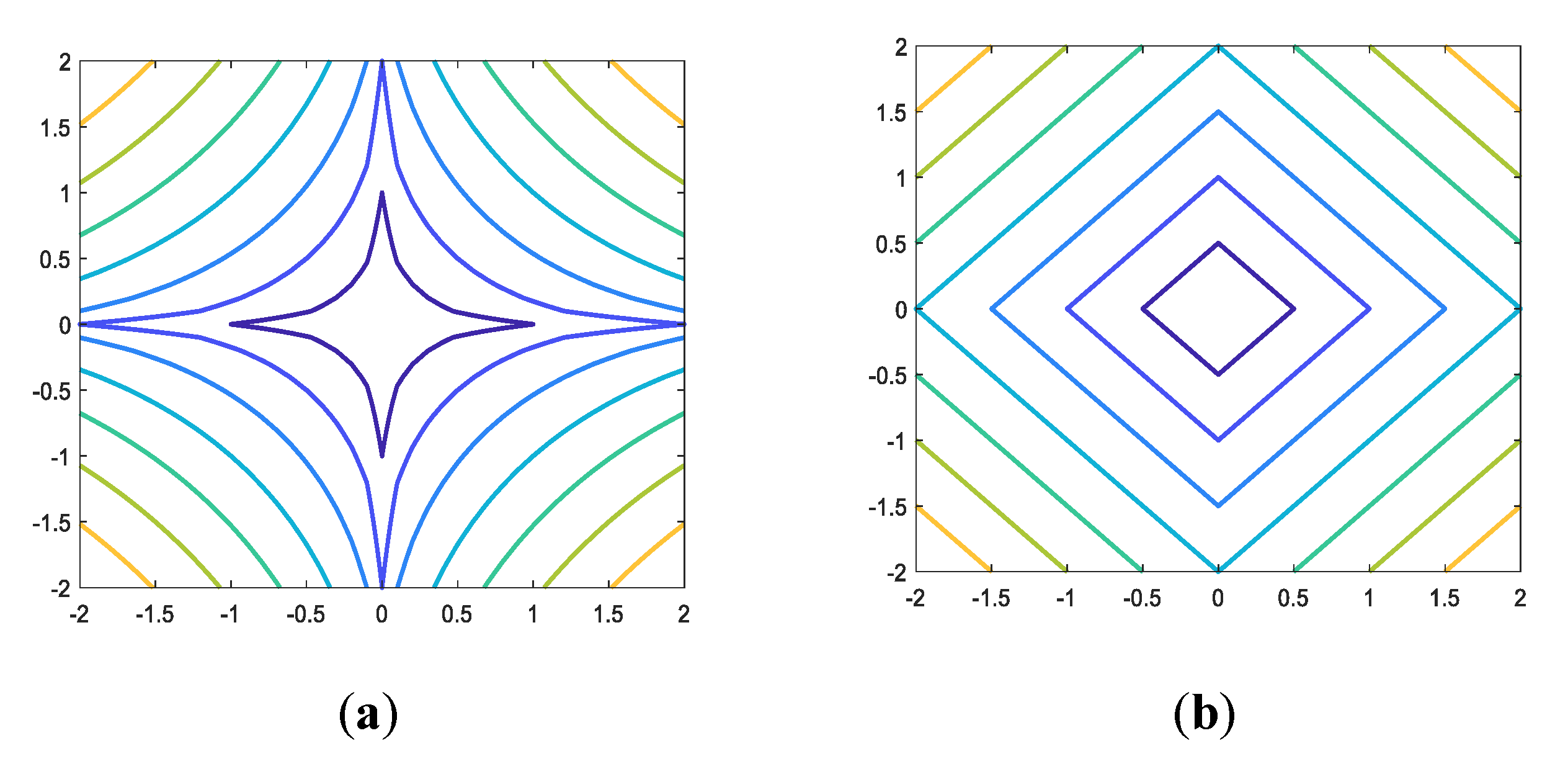
Figure 1. Contours of the Lp-pseudo-norm: (a) p = 0.5; (b) p = 1.
Algorithms 12 00221 g001
Figure 2. Feasible domain under the Lp constraint: (a) p = 0.5; (b) p = 1.
Algorithms 12 00221 g002
Figure 3. Images used in the simulation: (a) Fingerprint 256 × 256; (b) Butterfly 512 × 512; (c) Baboon 512 × 512; (d) Boat 512 × 512; (e) Bird 512 × 512; (f) Hill 512 × 512; (g) Truck 512 × 512; (h) Plane 512 × 512; (i) Satellite 512 × 512.
Algorithms 12 00221 g003aAlgorithms 12 00221 g003b
Figure 4. Effect of the regularization parameter μ on the experimental results. (a) Effect of μ on peak signal-to-noise ratio (PSNR) at noise levels 30%, 40%, 50%, and 60% with image “Boat”. (b) Effect of μ on PSNR at noise levels 30%, 40%, 50%, and 60% with image “Hill”.
Algorithms 12 00221 g004
Figure 5. Effect of the p and μ values on PSNR: PSNR (dB) for the recovery of image “Hill” degraded with a Gaussian blur kernel ( G , 7 , 5 ) and 30% impulse noise.
Algorithms 12 00221 g005
Figure 6. Comparison of the visual effects and PSNRs of image restorations of the “Boat” image degraded with a Gaussian blur kernel ( G , 7 , 5 ) and 30% impulse noise: (a) blurred image; (b) blurred image with 30% impulse noise; (c) fast total variation deconvolution (FTVd)-restored image; (d) total generalized variation (TGV)-restored image; (e) overlapping group sparsity total variation (OGSTV)-restored image; (f) proposed algorithm-restored image.
Algorithms 12 00221 g006
Figure 7. Local zoomed-in images from Figure 6 for better comparison: (a) selected region of the original image; (b) local zoomed-in image of the selected region; (c) FTVd-restored image; (d) TGV-restored image; (e) OGSTV-restored image; (f) proposed algorithm-restored image.
Algorithms 12 00221 g007
Figure 8. Comparison of the visual effects and PSNRs of image restorations of the “Fingerprint” image degraded with an average blur kernel ( A , 7 ) and 50% impulse noise: (a) blurred image; (b) blurred image with 50% impulse noise; (c) FTVd-restored image; (d) TGV-restored image; (e) OGSTV-restored image; (f) proposed algorithm-restored image.
Algorithms 12 00221 g008
Figure 9. Local zoomed-in images from Figure 7 for better comparison: (a) selected region of the original image; (b) local zoomed-in image of the selected region; (c) FTVd-restored image; (d) TGV-restored image; (e) OGSTV-restored image; (f) proposed algorithm-restored image.
Algorithms 12 00221 g009
Figure 10. Comparison of restored image details and the PSNRs for the “Butterfly” image degraded with a motion blur kernel ( M , 20 , 20 ) and 30% impulse noise: (a) selected region of the original image; (b) local zoomed-in image of the selected region; (c) blurred image; (d) blurred image with 30% impulse noise; (e) FTVd-restored image; (f) TGV-restored image; (g) OGSTV-restored image; (h) proposed algorithm-restored image.
Algorithms 12 00221 g010
Figure 11. Comparison of the visual effects and PSNRs of restored images for images degraded with different levels of motion blur and impulse noise.
Algorithms 12 00221 g011aAlgorithms 12 00221 g011b
Table 1. Values of p that give optimal peak signal-to-noise ratio (PSNR) values for different test images.
Noise LevelFingerprintButterflyBaboonBoatBirdHillTruckPlaneSatellite
30%0.300.450.500.350.500.550.500.550.75
40%0.300.450.500.350.500.550.500.550.75
50%0.300.450.500.350.500.550.500.550.75
60%0.250.500.500.350.500.550.550.550.75
Table 2. Numerical results of PSNR (dB), structural similarity (SSIM), and SNR (dB) for the recovery of nine test images degraded with a Gaussian blur kernel ( G , 7 , 5 ) and 30–60% impulse noise. FTVd—fast total variation deconvolution; TGV—total generalized variation; OGSTV—overlapping group sparsity total variation.
ImagesNoise LevelFTVdTGVOGSTVProposed
PSNRSSIMSNRPSNRSSIMSNRPSNRSSIMSNRPSNRSSIMSNR
Finger
print
3030.490.95021.9036.130.98027.3936.210.98027.6838.630.98930.08
4029.160.91319.8435.320.97626.7935.640.98126.437.440.98328.90
5028.370.86619.5133.040.95924.533.990.95724.5635.590.97027.05
6025.740.83116.2728.890.91520.3528.840.90619.3230.600.92322.07
Butterfly3028.210.89421.9630.370.91924.1730.840.93224.5932.170.94625.92
4027.360.87521.1129.580.90123.3330.460.92624.2130.990.93124.74
5025.420.82519.1728.450.86922.228.830.89522.4529.960.91223.71
6024.060.73414.4726.480.80420.2426.610.81820.2728.990.89822.75
Baboon3021.290.62815.8322.930.75617.4723.150.76517.6924.010.80618.55
4021.060.60815.6022.560.73017.1022.930.75617.4623.390.77917.93
5020.620.57215.1522.080.69316.6321.900.70216.4422.660.73817.20
6020.270.52514.4321.230.62715.7720.570.54615.1222.230.71016.77
Boat3027.250.84021.9229.050.89423.7129.450.90624.1131.460.93226.11
4026.490.80221.1628.330.87322.9929.060.89823.7130.280.91424.94
5025.650.78920.3027.250.83921.9127.230.83621.8828.470.88423.12
6023.900.75618.5625.130.76619.8026.300.78021.0627.370.84921.78
Bird3031.030.91421.9732.820.93423.7633.490.94724.4334.540.95725.47
4029.710.89020.6531.840.91522.7733.030.94123.9733.390.94324.32
5026.730.83117.6729.460.87420.3930.450.88221.3832.310.93023.24
6022.750.72213.6926.990.79717.9327.850.81318.7729.690.89820.62
Hill3028.240.85921.8730.270.89823.9130.710.90824.3531.980.92525.62
4027.240.83120.8829.480.87823.1130.290.89923.9330.940.90924.57
5025.570.80219.6828.390.84522.0328.250.86521.9229.720.88723.36
6024.870.76018.5126.160.77319.7927.030.84520.6928.520.85521.74
Truck3029.500.88722.2332.790.92625.5233.480.93926.2234.220.94626.96
4028.700.82821.7331.850.90824.5833.060.93225.7933.140.93325.87
5027.260.79419.9930.420.87323.1531.170.90523.9032.500.92325.23
6026.130.62019.1829.060.86021.8030.480.86523.1131.050.90323.79
Plane3032.370.90229.1833.960.94830.7736.330.97533.1536.230.97433.05
4031.680.89828.4933.000.92929.8235.200.96131.3735.300.96532.11
5030.420.83127.2431.430.89228.2532.710.90129.5233.900.95130.72
6027.900.73024.7229.730.76426.0430.070.80526.8931.960.92728.78
Satellite3031.800.92518.1234.170.95920.4936.970.98923.2036.540.98523.05
4030.380.91016.7033.390.94519.7236.000.98322.3235.760.98022.08
5029.080.88315.4131.370.91017.7032.320.92618.6432.610.97518.92
6027.990.83014.3129.540.85515.8630.050.90416.3830.210.94416.72
Table 3. Numerical results of PSNR (dB), SSIM, and SNR (dB) for the recovery of nine test images degraded with a Gaussian blur kernel ( G , 15 , 5 ) and 30% impulse noise.
ImagesDegrada
-tion
FTVdTGVOGSTVProposed
PSNRSSIMSNRPSNRSSIMSNRPSNRSSIMSNRPSNRSSIMSNR
FingerprintBlur:
( G , 15 , 5 ) Noise level:
30%
27.310.87718.7829.890.93521.3630.090.93421.5530.720.97022.18
Butterfly24.910.70518.6726.960.86120.7227.050.86420.8027.470.87321.22
Baboon19.890.48114.4320.990.59715.5321.090.60315.6221.720.64516.27
Boat24.730.67919.2025.630.81520.2926.370.83521.0226.860.85121.82
Bird28.150.74119.0829.600.88520.5429.810.89220.7530.050.90620.91
Hill25.980.69019.6827.370.83021.0127.410.83221.0528.010.84021.65
Truck27.560.70720.2929.420.86222.1629.570.86622.3130.300.87223.01
Plane29.760.81526.5830.670.90427.6531.340.93828.1531.820.94828.64
Satellite28.200.82114.5229.660.90015.9831.470.96317.7931.390.96217.71
Table 4. Numerical results of PSNR (dB), SSIM, and SNR (dB) for the recovery of nine test images degraded with an average blur kernel ( A , 7 ) and 30–60% impulse noise.
ImagesBlur SizeNoise LevelTGVOGSTVProposed
PSNRSSIMSNRPSNRSSIMSNRPSNRSSIMSNR
Fingerprint ( A , 7 ) 3036.460.98327.9136.730.98029.1938.310.98929.77
6028.740.90520.2029.300.90721.2430.110.91021.57
Butterfly3030.400.91824.1530.990.93324.7432.210.94725.97
6025.830.78419.5926.450.80320.6628.590.89522.35
Baboon3023.010.76117.5423.290.77817.8324.110.81418.65
6021.140.62215.6821.510.65716.1022.310.71516.85
Boat3029.110.89423.7729.600.90724.2631.500.93326.16
6025.110.75519.7726.240.77620.5227.220.85521.88
Bird3032.750.93323.6733.530.94824.4734.530.95725.46
6027.050.78517.9929.060.85320.3530.190.89921.13
Hill3030.330.89923.9730.850.91024.4932.070.92725.71
6025.960.75719.6026.100.76220.0727.960.85221.60
Truck3032.790.92525.5233.610.94026.3434.320.94727.06
6027.250.78019.9730.280.84822.3231.380.90424.12
Plane3033.870.94530.6836.450.97533.2736.370.96933.08
6028.150.79324.9731.870.92228.6932.310.92629.13
Satellite3033.950.95620.2836.850.98923.1836.520.98123.10
6028.060.81414.3828.520.93314.8428.540.93314.87
Table 5. Numerical results of PSNR (dB) for the image restoration test conducted on four test images degraded with different levels of blur and impulse noise.
ImagesBlur SizeNoise LevelFTVdTGVOGSTVProposed
Baboon ( M , 10 , 10 ) 3021.792124.010022.064724.8964
4021.178522.902023.218324.3687
( M , 20 , 20 ) 3021.086323.095822.840223.6167
4020.772122.455422.352223.2369
Butterfly ( M , 30 , 30 ) 3026.061628.707028.467129.3110
4025.360227.925027.882028.9013
5024.240626.864327.226928.3973
6022.479725.225026.426427.7279
Bird ( M , 20 , 20 ) 3030.061831.780532.559633.3166
4028.734130.319531.878832.6383
5026.273228.210631.153831.7443
6022.953625.254330.168030.3756
Truck ( M , 20 , 20 ) 3030.317731.808732.349533.3499
4029.138130.315431.759232.7189
5027.526028.409331.110431.9235
6024.701325.222030.064230.7173
Table 6. Image restoration time (s) of the degraded test images with different levels of blur and impulse noise.
ImagesBlur TypeNoise LevelFTVdTGVOGSTVProposed
Fingerprint
256 × 256
( G , 7 , 5 ) 300.861.470.811.19
( A , 7 ) 400.921.480.981.17
( M , 20 , 20 ) 300.811.471.091.22
( M , 20 , 20 ) 600.841.481.471.17
Plane
512 × 512
( G , 7 , 5 ) 303.286.036.205.31
( A , 7 ) 403.426.175.985.36
( M , 20 , 20 ) 303.616.286.785.33
( M , 20 , 20 ) 603.276.364.165.36
Satellite
512 × 512
( G , 7 , 5 ) 303.367.113.115.27
( A , 7 ) 403.506.202.665.34
( M , 20 , 20 ) 303.316.223.595.16
( M , 20 , 20 ) 603.236.234.095.14