1. Introduction
As one of the three artificial boards, particleboards can be made of chipped broken wood or wheat stalk, rice straw, bamboo, etc. The basic material used for particleboards is very small and can come from different sources. Particleboards are widely used in many fields due to their advantages of low production cost, high hardness, and wide market availability. Since the 21st century, energy conservation has become an important indicator of the technical level of industrial production. The problem of poor forest resources and low forest coverage has meant the industrial production of particleboards has become an important method to make up for this situation.
At present, in the field of surface defect detection of particleboards, most production lines are technologically backward, with some even relying on artificial, visual inspection. This method is not only inefficient but also costs a lot of manpower, and the results are not exact enough.
In recent years, many scholars have made contributions to improve the technology of particleboard production line, including those involving technical fields such as impact resistance and internal bonding strength [
1,
2,
3,
4,
5,
6,
7,
8,
9]. In Reference [
1], samples of high-density homogeneous particleboards of sugarcane bagasse and castor oil polyurethane resin were manufactured and subjected to low-velocity impacts using an instrumented drop weight impact tower and four different energy levels. Reference [
3] evaluated the physical and mechanical properties of particleboards manufactured from a mixture of sycamore leaves and wood particles. In Reference [
6], the effects of grit sizes of sand belt, feeding speed, and the feed power of the heads of the sander on surface roughness of the particleboard panels were investigated. Reference [
7] evaluated the physical, mechanical, and durable properties of sorghum bagasse particleboards (SBP), which are layered by several materials. Despite these numerous studies, the detection of surface defects has seldom been reported. In the field of automatic detection of surface defects, some scholars have studied detection methods for the characteristics of steel, glass, and other materials [
10,
11,
12,
13,
14,
15,
16,
17,
18,
19], but few have studied the surface defect detection technology on particleboards. In Reference [
10], classical convolutional neural networks (CNNs) trained in pure supervised manner was used to detect defects on steel surfaces. The defects were identified by the reflection of light on the steel surface owing to the good reflectance of steel materials. Although this method can effectively identify steel surface defects, it takes a long time to calculate. Moreover, it is not suitable for rough surface materials, such as particleboards, as it cannot detect defects by reflective characteristics. A detection algorithm for the recognition and segmentation of defects in mobile phone screen glass (MPSG) was proposed in Reference [
12]. The combination of subtraction and projection (CSP) was used to identify defects on the MPSG image, which could eliminate the influence of fluctuation in ambient illumination. Reference [
17] proposed an efficient similarity measure for the detection of surface defects in printed circuit boards (PCB). The method could measure the similarity between the scene image and the reference image of PCB surface without the need to compute image features such as eigenvalues and eigenvectors. The method proposed in Reference [
18] was aimed at improving quality control in the ceramic tile industry. An automated inspection system for ceramic tile based on image processing techniques was used to detect edge damages and middle cracks on the surface of the tile. Reference [
19] proposed a method for detecting defect on air-bearing surfaces (ABS), which has variance luminance intensity. The co-occurrence matrix was used to avoid the variance intensity of ABS images. However, these methods are only suitable for the detection of small defects. When applied to the detection of surface defects in particleboards, a large number of small wood chips on the surface of the board may cause serious false detection. Reference [
15] proposed a method based on thresholding segmentation to detect surface defects in a glass substrate. A straight-line intercept histogram was established directly from the two-dimensional information of an image, and the Otsu criterion was then used to find the best intercept threshold from the one-dimensional histogram. However, this method can only detect the surface of the glass substrate by taking photos under the static state, and it cannot realize dynamic detection on the production line.
Through the study of existing technologies, the aim of this paper is to examine the problem of detecting surface defects in particleboards.
In the whole production process of particleboards, the board is always in motion in the production line, and the surface defects are mostly exposed shaving defects. In view of this situation, we adopted the moving target tracking technology and the image segmentation technology to achieve image capture, extraction, and detection of surface defects in particleboards, including defects of different sizes and shaving defects with different depths. The main contributions of this study can be summarized as follows:
(1) The KCF moving target tracking algorithm was used to track surface defects in particleboards in the production line, and the forward–backward error was introduced to reduce the tracking error using the median flow method.
(2) The motion targets of each frame in video sequence were extracted using the edge detection method to obtain more complete and accurate characteristic data of the moving target.
(3) According to the extracted defect images, various defect characteristic parameters were calculated, and the surface defect level of the particleboard was evaluated using the fuzzy pattern recognition method.
The rest of the paper is organized as follows.
Section 2 introduces the KCF target tracking algorithm, which was used to capture the surface defects in the particleboard.
Section 3 introduces the samples and equipment used in the experiment. In
Section 4, the tracking and detection results of the surface defects are given.
Section 5 gives the calculation of the defect characteristic parameters according to the extracted defect images. The defects are also analyzed using fuzzy pattern recognition. Finally, the conclusions of the work are drawn in
Section 6.
2. Algorithm Theory
2.1. The KCF Target Tracking Algorithm
The kernel correlation filter has been widely used in the field of moving target detection and tracking since it was first proposed in 2014 [
20]. KCF is a discriminative tracking method that mainly uses the given samples to train a discriminative classifier, which can distinguish between targets and backgrounds. Circulant matrices are used to translate and scale the samples, and the discrete Fourier transform (DFT) is used to accelerate the algorithm.
Considering an
vector and
representing a line of the target area image as the base sample, in order to get more samples to train the classifier, we can use a cyclic shift operator
to perform one-dimensional translations of
.
is a
matrix.
Due to its cyclic property, all samples obtained after transformation can be expressed by the following equation:
Equation (2) can be written in matrix form as follows:
Equation (3) represents the form of circulant matrices [
21]. The elements in X depend on vector x, while DFT makes the matrices diagonal [
22]. Equation (3) can be expressed as follows:
where
is the DFT constant matrix, and
denotes the DFT of
, i.e.,
.
Circulant matrices combined with DFT can generate a large number of samples for classifier training in a stable and effective way, thus ensuring the accuracy of tracking results.
The “kernel trick” can be used to turn a linear mapping problem to a nonlinear kernel space and turn the calculation of low-dimensional space mapping to high-dimensional kernel space. The inseparable problem in low-dimensional space will become linearly separable in high-dimensional space, and we can realize an efficient training of the classifier [
23].
We can define the
kernel matrix as follows:
where
is the kernel correlation of the base sample
and base patch
.
According to the regression function,
can be given as follows:
where
is the regression coefficient; the value range of
is
; and
is the element of a
matrix
, which denotes the dot products between
and
.
We can compute the regression function for all candidate patches with the following equation:
Diagonalizing Equation (7), we obtain the following:
It is obvious that is a linear combination of the neighboring kernel values from , weighted by the learned coefficients . As this is a filtering process, it can be better expressed in the Fourier domain.
When the kernel function training is complete, the new sample will map to the kernel space directly. Using the trained function to calculate the value for all positions, the location of the target can then be quickly detected.
Although KCF can perform well in both tracking effect and tracking speed, it also has a limitation in that it is not free to change the size of the target tracking boxes; this means tracking can be easily disturbed when the target is covered. However, for the detection of surface defects in particleboards, it is almost impossible that the defect targets will be deformed or covered, thus the imperfection of the algorithm will not have a negative impact the final tracking effect. Moreover, the advantage of fast tracking speed of the algorithm can fully meet the requirements of the running speed of a normal production line, ensuring real-time performance.
2.2. The Median Flow
The median flow is derived from the tracking module in the tracking–learning–detection (TLD) algorithm [
24,
25,
26,
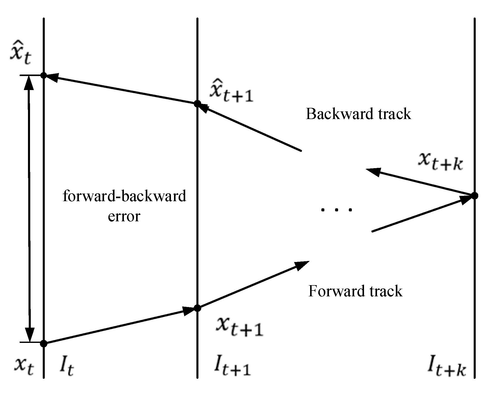
27]. According to the principle that a good tracking algorithm should have forward–backward consistency, i.e., in a chronological or antichronological order, the tracking results should be the same. We can define the forward–backward (FB) error of an arbitrary tracker as follows:
where,
denotes the processed image sequence;
is the position of the feature point
at time
;
and
denote the chronological order and the antichronological order tracking results, respectively; and
is the number of the current image frame.
Equation (9) shows that the FB error of a tracker is essentially the Euclidean distance between the initial position
and the predicted position
of the feature point
. The calculation diagram of FB error is shown in
Figure 1.
In the process of tracking, the FB errors of each feature point are calculated, and the point whose FB error is less than the median value of the sum of the total FB errors is taken as the effective tracking feature point. Finally, according to the coordinate changes of these points, the position of the target boundary box in the image at time
can be calculated.
where
denotes the change rate of the distance between point
and point
in the two adjacent frames;
denotes the average change rate of
; and
denotes the size of the target boundary box in image
, which is the number t frame image in the video sequence.
In this study, the median flow algorithm was used to amend the tracking results of the KCF to make the tracking results more accurate and ensure the reliability of subsequent calculation results of the target defect parameters.
2.3. Sobel Edge Operator
After the defect targets are captured by the tracking algorithm, their images will be extracted by edge detection. In this study, the defect targets were separated from the background by the Sobel edge operator.
The Sobel edge operator has two
templates. Considering
as the original image, then image
, which is detected vertically, and image
, which is detected horizontally, can be expressed as follows:
The value of gradient can be expressed as follows:
The direction of gradient can be expressed as follows:
The Sobel edge operator can make a further weighted adjustment to the undesirable segmentation results according to the pixel position. This process can alleviate the edge blurring and improve the quality of the segmentation results.
4. Tracking and Detection Experiment
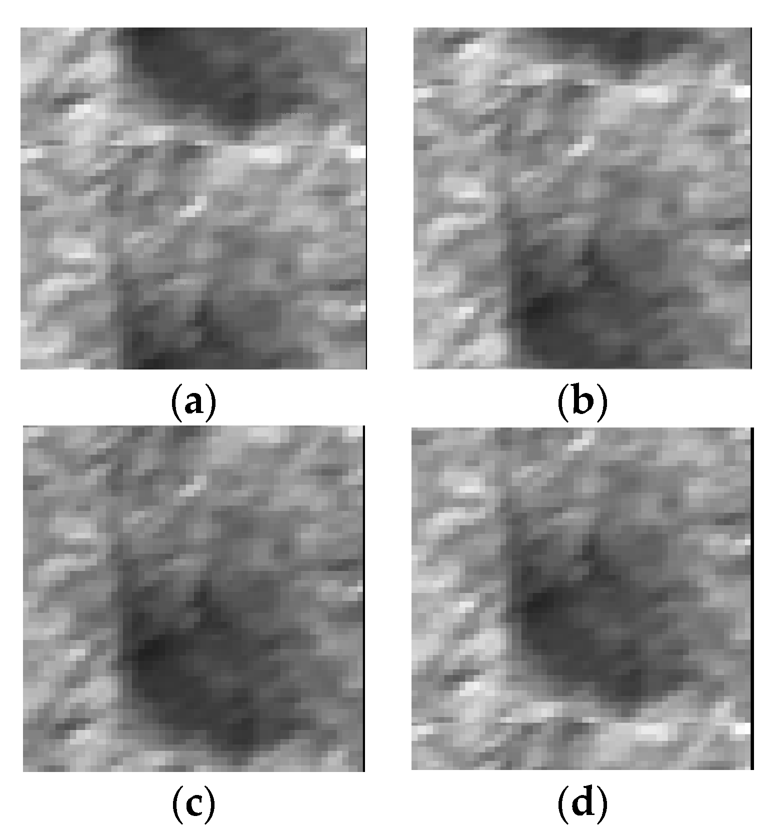
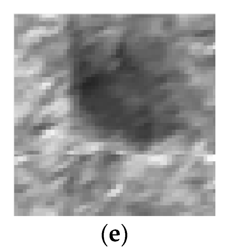
In this study, three particleboards with different degrees of surface defects were selected as experimental objects, and a total of five exposed wood shaving defects on their surfaces were tracked. The experimental particleboards were numbered
. The surface defects, shown in
Figure 3, were numbered
. Among them, defect
and
were in board
, defect
was in board
, defect
and
were in board
. The surface quality grade on the production line was first-class for board
, second-class for board
, and third-class for board
. (Boards of class 1 are excellent, class 2 are medium, and class 3 are inferior.)
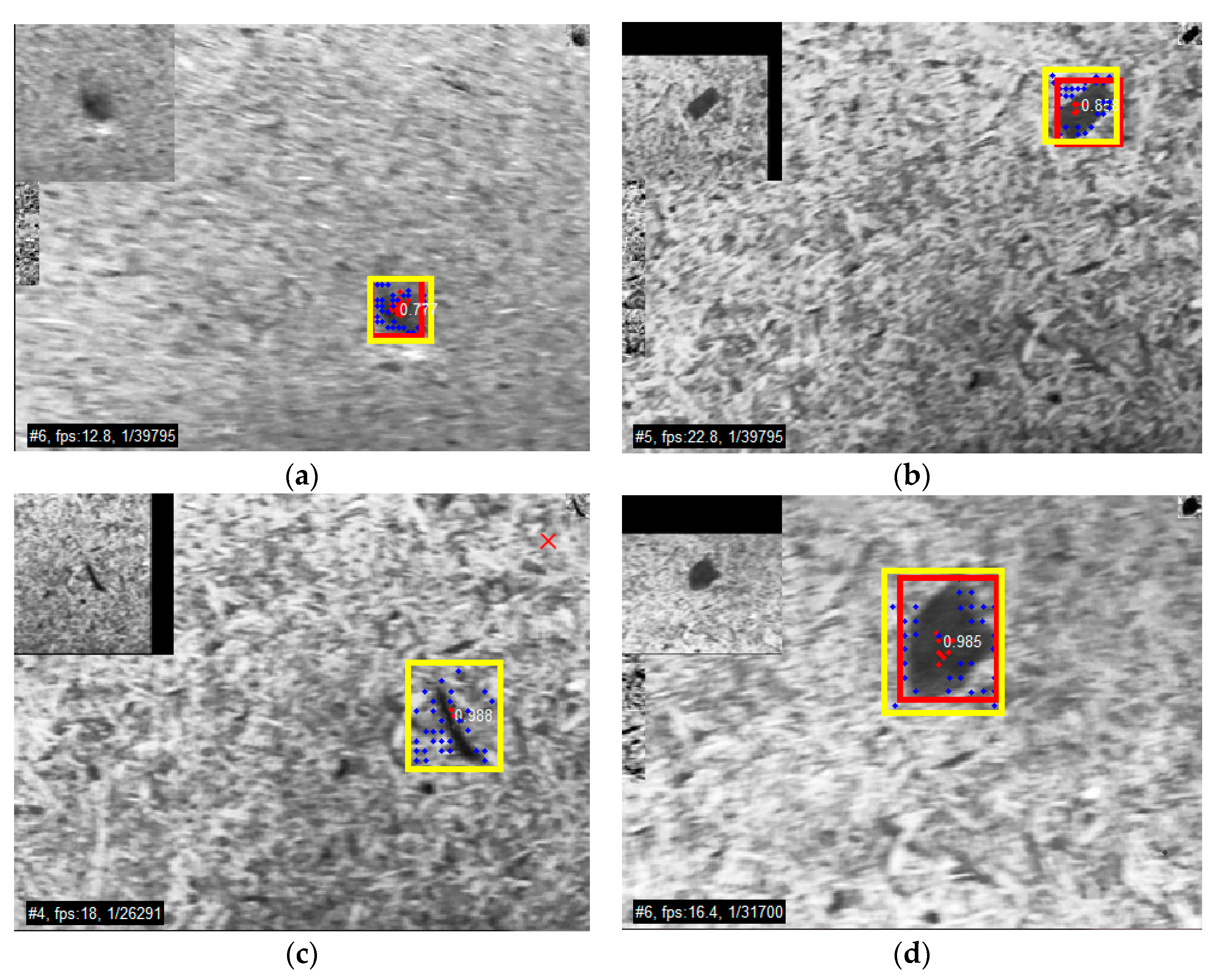
A comparison between the tracking results of the improved KCF algorithm with the median flow correction and the TLD algorithm is shown in
Figure 5.
In
Figure 5, the red target tracking box denotes the tracking results of KCF, and the yellow target tracking box denotes the tracking results of TLD. The "x" in the upper right corner denotes the loss of the tracking target of the corresponding algorithm.
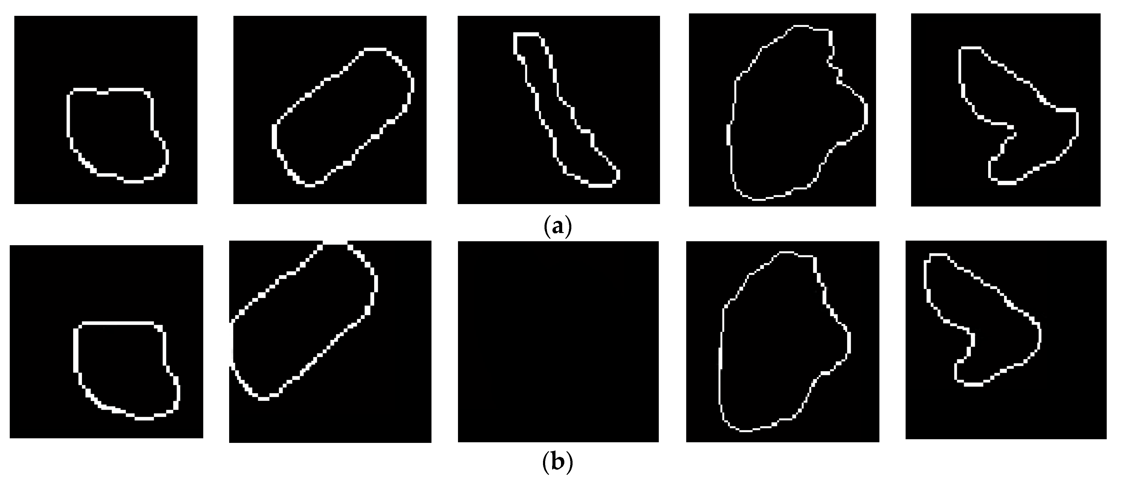
The edge detection results of defect images in the target tracking box using Sobel operator is shown in
Figure 6. The result vacancy represents the loss of target in the tracking process.
It can be seen from the tracking and detection results that the TLD lost several targets in the process of tracking, while the KCF hardly lost any of the targets.
The computation time of each defect target tracked by KCF was less than 0.1 s, which can fully meet the real-time requirements of the particleboard production line.
5. Calculation and Analysis of Defect Characteristic Parameters
5.1. The Area of Defect Targets
By calculating the number of pixels inside the edge, we can obtain the area of the defect target detected in the current frame image. The larger the area, the more serious is the defect damage. In the tracking and detection process of a single defect, a defect area value is obtained for each frame of image, and the average value
is taken as the final defect area.
Table 1 shows the results of defect area calculation of surface defect targets.
5.2. The Depth of Defect Targets
The depth of defect targets d can be defined as the gray average difference of the target image area and the background image area. It can be calculated as follows:
where
and
denote the gray average of defect target area and background area, respectively;
is the gray value of pixel
;
denotes the entire target area;
denotes the total number of pixels in the image; and
denotes the number of pixels in the target area.
In the tracking and detection process of the defect, we can get a value of defect depth in each frame of image, and their average is also taken as the final value of
. The greater the value of defect depth
, the more serious is the defect damage.
Table 2 shows the results of defect depth calculation of surface defect targets.
5.3. The Number of Surface Defects
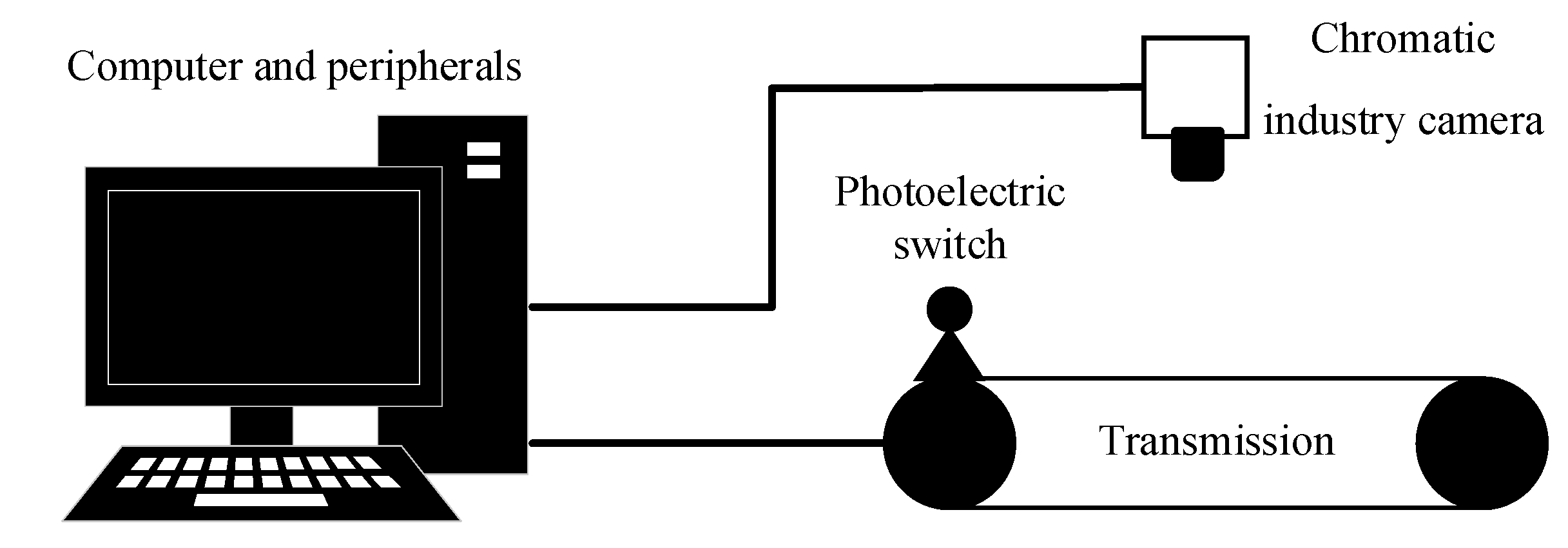
When the particleboard is transported on the transmission, the photoelectric switch can give the start or end signals when the board enters or leaves the camera view. The program counts the number of defects detected during each group of start–end signals and takes it as the number of defects on each particleboard. According to this, there were two defects in board , one defect in board , and two defects in board .
5.4. The Analysis of Surface Defects
Fuzzy pattern recognition is used to analyze surface defects in particleboards according to the obtained defect characteristic parameters [
28,
29,
30,
31]. Considering the feature of the characteristic parameters, the method of group identification was adopted in this study to solve the problem, while the Hamming distance, Euclid distance, and dose-approximation value were selected as the evaluation indexes.
Considering
and
are the fuzzy subsets on the domain
, the Hamming distance between the fuzzy sets
and
can be expressed as follows:
The Euclid distance between fuzzy sets
and
can be expressed as follows:
and
are essentially
vectors. The inner product of
and
can be expressed as follows:
The outer product can be expressed as follows:
The dose-approximation value of
and
can be expressed as follows:
It can also be written as follows:
The final pattern recognition result is obtained according to the principle of proximity selection. Considering are the fuzzy models on domain , and is the object to be identified, if there is , will be considered to belong to fuzzy model .
In this study, the surface defects of the particleboard were divided into
,
, and
grades. The required indexes are shown in
Table 3.
From
Table 3, we can obtain that the standard fuzzy sets of the first-class, second-class, and third-class boards were
,
, and
, respectively.
The surface quality indexes of the experimental particleboards are shown in
Table 4.
From
Table 3, it can be obtained that the standard fuzzy sets of the first-class, second-class, and third-class boards were
,
, and
, respectively.
The Hamming distance, Euclid distance, and dose-approximation values between the experimental boards and standard boards are shown in
Table 5,
Table 6 and
Table 7, respectively.
According to the principle of proximity selection, the following conclusions can be drawn from the three evaluation indexes of fuzzy pattern recognition: Particleboard was the second-class board, board was the first-class board, and board was the third-class board.
As can be seen from the above experimental results, the artificial detection not only had undetected errors but also failed to accurately give the characteristic parameters of the defects. In the experiment conducted with TLD, a defect in board D was undetected, and the calculation error of the defect damage degree was large, leading to reduced accuracy of the final analysis results. In comparison, the KCF-based detection algorithm proposed in this paper could accurately capture the defect targets on the surface of the particleboards. The calculation results of the defect characteristic parameters had a high accuracy, and the analysis result was in line with the actual situation.
The process of the detection of surface defects in particleboards and surface quality evaluation is shown in
Figure 7.


