Data Analysis, Simulation and Visualization for Environmentally Safe Maritime Data

Abstract

Marine transportation in Aegean Sea, a part of the Mediterranean Sea that serves as gateway between three continents has recently seen a significant increase. Despite the commercial benefits to the region, there are certain issues related to the preservation of the local ecosystem and safety. This danger is further deteriorated by the absence of regulations on allowed waterways. Marine accidents could cause a major ecological disaster in the area and pose big socio-economic impacts in Greece. Monitoring marine traffic data is of major importance and one of the primary goals of the current research. Real-time monitoring and alerting can be extremely useful to local authorities, companies, NGO’s and the public in general. Apart from real-time applications, the knowledge discovery from historical data is also significant. Towards this direction, a data analysis and simulation framework for maritime data has been designed and developed. The framework analyzes historical data about ships and area conditions, of varying time and space granularity, measures critical parameters that could influence the levels of hazard in certain regions and clusters such data according to their similarity. Upon this unsupervised step, the degree of hazard is estimated and along with other important parameters is fed into a special type of Bayesian network, in order to infer on future situations, thus, simulating future data based on past conditions. Another innovative aspect of this work is the modeling of shipping traffic as a social network, whose analysis could provide useful and informative visualizations. The use of such a system is particularly beneficial for multiple stakeholders, such as the port authorities, the ministry of Mercantile Marine, etc. mainly due to the fact that specific policy options can be evaluated and re-designed based on feedback from our framework.

1. Introduction

Ships’ traffic is the supreme central factor of maritime shipping safety. The rising number of vessels and their sizes, together with cargo type, is related to increased likelihood of accidents including fires, explosions and losses of life and catastrophic impact on the environment. Such negative effects increase awareness of government bodies, industry sectors and society on the importance of risk assessment. To assess such a risk, domain experts need to know and understand how marine traffic behaves. Traffic trend modeling is an input of high value to construct robust risk assessment policies. AIS (Automatic Identification System) provides a great opportunity for traffic monitoring but also for discovering basic processes which govern the domain of marine traffic in given areas of interest.

One of the main difficulties posed by marine traffic engineering is to determine the optimum parameters of existing or newly constructed parts of the waterways. Depending on the type of waterway parameters that can be obtained are, for example, density of ships per time period, changes of speed when conditions change on neighboring areas, level of cargo hazard in combination with sea water conditions, etc. Such factors are usually obtained by either an inexpensive but less accurate analytical method or by a more expensive but accurate simulation method [1].

1.1. ICT and Maritime Data Engineering

The advances of Information and Communication Technology (ICT) could certainly be exploited for both real-time monitoring and alerting functionalities and for exploring patterns of past data behavior and obtaining knowledge about their properties with the forecasting ability into mind. The AIS system, along with other sensor data such as radar and GPS can fully support the above operations.

External conditions on the sea also play an important role to maritime traffic engineering. Sea and weather conditions are often one of the main causes of marine accidents, also deteriorating any potential rescue plan. In the Mediterranean Sea, on the 8th of December 1966, SS Heraklion was overwhelmed by heavy seas in the Aegean Sea whilst on passage from Crete to Piraeus and capsized. Of the 281 people on board only 47 survived [2]. A more recent incident (luckily without casualties) happened on the 8th of February 2016, the vessel MV Epsilon, severe weather conditions resulted in its heavy roll during a turn and mass shifting of its cargo, causing damages and some injuries [3]. Some cases from marine accidents in the Artic region are also presented in [4].

ICT has portrayed significant improvements towards this direction as well, by deploying real-time monitoring or modeling systems that constantly provide software agents with meteorological and sea conditions for a given location. Big data and data mining have also been developed into one of the fastest-growing areas in ICT. The vast amounts of generated data from the marine traffic domain and from other sources as well, requires sophisticated solutions when handling, collecting and analyzing big data to extract meaningful knowledge.

A large variety of data mining platforms have been introduced, requiring less programming and deploying effort from the user’s perspective than ever. Furthermore, web technologies have progressed to a phase that nowadays, one can use any type of electronic device (such as smartphones, tablets, PCs) and gain full access to distributed data, hybrid methods and sophisticated visualization outcomes. Based on all the above arguments, it is mature to state that the proposed work, is utilizing all of the aforementioned ICT services in order to ensure effective modeling, analysis and simulation of marine traffic data and provide experts with useful insight on current but also future trends and patterns.

1.2. Factors That Raise Marine Traffic Engineering Awareness

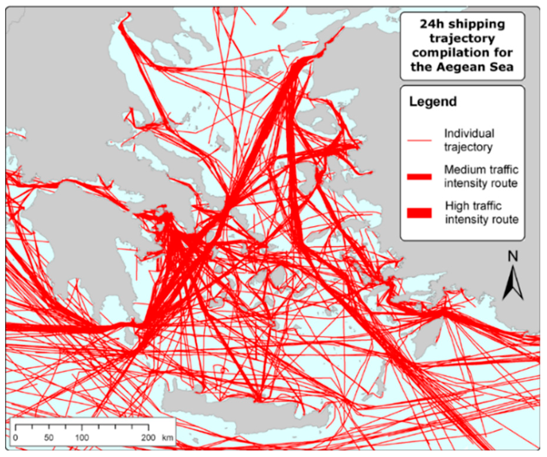
The current work focuses on Aegean, an archipelago of the Mediterranean Sea which connects three continents, such as Europe, Asia and Africa. Aegean Sea is an area in which shipping traffic has increased dramatically. This increasingly heavy traffic brings a great risk of maritime disaster, which could have long lasting environmental and socio-economic impact. The Aegean archipelago has the highest accident rate in the Mediterranean.

The development of shipping, the international trade and tourism relations but most importantly the geographical location of the Aegean contributes to increased shipping traffic in the area. Every day, hundreds of ships are cruising the waters of the Aegean to transport people, goods, materials and fuel to and from various regions of Greece, Cyprus, Egypt, Turkey and the Middle East. The following factors need to be identified to provide a qualitative insight on marine engineering awareness.

1.2.1. Sea Traffic

The maritime traffic in the Mediterranean Sea has increased dramatically in recent years due to technological advances in vessels, which have greatly improved the speed, capacity and size. In addition, tourist cruisers choose the eastern Mediterranean for the conduct of the cruise, offering economic and tourism boom in the region. However, the shipping around the area is not thoroughly controlled and lots of dangers are lurking.

Despite the small size of the Mediterranean Sea in relation to the area covered by the Earth, it is the home for approximately 14–18% of marine species worldwide and about ¼ of organisms that lives in the Mediterranean considered endemic. Characterized by a large number of small islands and narrow channels, where a lot of protected species can find appropriate conditions to survive such as sea turtles, seals, marine mammals and sharks. Consequently, it is important to protect and preserve the eastern Mediterranean area from the devastating impacts of uncontrolled shipping [5].

1.2.2. Accidents and Hazards

The Aegean Sea has the highest accident rate in whole the Mediterranean region. According to a recent survey conducted by “Archipelagos”, (a Greek institute of marine conservation) in three key vessel passages of the Aegean Sea, it was observed that about 65% of the moving vessels were cargo ships, 21%, were tankers and only 5% were passenger ships. Furthermore, it was observed that a large number of vessels sailing under “flags of convenience”, about 16%, increased chances of an accident.

Lack of Designated Shipping Lanes

The lack of regulated waterways allows vessels to moving at will, without any control and safe shipping lane policy, as illustrated in Figure 1. The enforcement of designated shipping lanes through the most suitable routes has been proven as a factor of reducing the number of accidents in other seas globally, therefore reducing the chance of ecological and socio-economic disaster.

1.2.3. Impact of Maritime Accidents

A maritime accident would cause irreparable damage to the ecosystem of the Aegean Sea and socio-economic losses to both Greece and Turkey. In the past, within the Aegean Sea, several accidents have occurred, causing irreparable damage to the environment. The sinking of the tanker “Irene Serenade” resulted in a crude oil spill of 120,000 tons near the touristic ad historic Greek city of Pylos. The sinking of the cruise ship “Sea Diamond”, which happened in the Greek island of Santorini in 2007, was a marine accident that cost two lives, about 7.2 million Euros to the Greek state and caused major ecological disaster in the Aegean Sea after spilling 250,000 liters of diesel [6]. Nowadays, 11 years later, the ship continues to contaminate the area of the continuous leakage of oil and a series of toxic pollutants such as asbestos and mercury, as the hull of the ship is decomposing. Studies have shown that these contaminants can pass into the human food chain, since local fishes caught for consumption.

1.3. Research Questions

Based on the above arguments, the present work deals with three research questions:

• RQ1: How to incorporate various heterogeneous data sources about marine traffic, vessel information and sea conditions towards modeling and understanding potential hazardous situations.
• RQ2: How to exploit historical data towards creating a simulation tool for inferring about future situations under conditions of uncertainty.
• RQ3: How to create useful visualization and insights for the domain, in order to help experts formulate policies, regulations, reform emergency plans, etc.

2. Related Work

In order to be inline with the aforementioned research questions, the present section discusses recent works in exploitation of AIS data for identifying maritime routes, analysis and visualization of historical data for simulation purposes and risk models for marine traffic.

The work of [7] shows that the combination of automated grouping of AIS data opens up a range of possibilities for analysis of ship traffic and maneuvering from simple statistical studies of current traffic to the inference of a prototypical voyage plan for a group of ships. In [8], the authors presented a space-use method, which is available and popular in the domain of movement ecology, in an attempt to analyze Principal Fairways (PF). The used AIS data together to bathymetric data in order to identify when and where strait corridors are used by transit-passage vessels. They argued that this method has certain value in maritime risk assessment and waterway planning in a specific strait. In [9], it was reported that AIS data could be used as an important tool for a wide range of industries and stakeholders of the marine domain such as spatial planning, developments and local marine industries (e.g., fisheries). He demonstrated a procedure for processing, analyzing, and visualization of AIS data with example outputs and their potential uses. The extracted knowledge resulted in the development of tools that performed density mapping, vessel tracking, interpolations of vessel dimensions, and ship type analysis. The dataset was subdivided according to its sector and was mapped into data packets which could also be analyzed over time. Additional uses of AIS data were proposed to monitor invasive non-native species, fisheries, and general statistics. Similar exploitation of AIS data is also presented by [10]. In this work, an AIS data warehouse environment is built in order to be referenced by port development planning, traffic forecasting, navigation safety assessment, and policy-making decisions.

In the analytical review paper of [11], it is stated that AIS data have proven to be practical and useful for activities ranging from basic traffic management, strategic planning, simulation-based training, analysis of various risks in terms of human, environmental, and economic loss, decision-making in the contexts of safety and security at sea. A noteworthy remark is that amongst the reviewed publications, a major common point was identified: that the information service is strongly dependent on the quality of AIS information and intelligent applications for information processing, integration, and presentation. In this context, it has also been demonstrated that AIS alone has never been sufficient to describe a full, comprehensive maritime picture.

As regards to the analysis and visualization of historical data records as basis for simulation under uncertainty, we would like to refer to the works of [12,13]. The former studied wintertime navigational accidents in the Northern Baltic Sea. For cases with no AIS information, they used simulation techniques from video analysis. Together with visual data mining, a well-known method for its utility in obtaining qualitative knowledge from data sources through a combination of visualization techniques and human interaction with the data, they managed to analyze accidents that occurred between 2007 and 2013. The results, as claimed by the authors, could be primarily useful for improving risk analyses focusing on oil spill risks in winter conditions and for developing realistic training scenarios for oil spill response operations. The latter work focused on extreme weather factors and their correlation with commercial fishing operations. Based on data obtained from the area of Atlantic Canada, regression analysis demonstrated the existed of strong relations between the studied weather factors and fishing activity incidents.

Some interesting research in the field of simulation of marine traffic is presented in [14]. A probabilistic model is used to analyze the risk of two frequent types of marine accidents, such as collision and grounding. Their attention is specified upon oil tankers since they pose the highest environmental risks. The probability of vessel colliding is assessed in terms of a minimum-distance-to-collision-based model. The model defines the collision zone using a mathematical ship motion model and considers the traffic flow to be a non-homogeneous process. Similar approach is followed for the probabilistic assessment of grounding. Furthermore, in the work of [15], the authors presented a simulation model that attempts to assess the potential impact of deepening the terminals and ports of Delaware River and Bay areas, by considering multiple parameters such as tide, navigation, terminal and anchorage rules as well as vessel profiles.

Concerning risk analysis, a solid review article by [16] emphasized on the catalytic influence of solid scientific basis in qualifying risk measurements. They stated that many of their studied applications and methods lack clarity about foundational issues concerning the scientific method of risk analysis. Definitions for key terminology are often lacking, perspectives are not introduced and little attention is given to the scientific approach underlying the analysis. Furthermore, another important conclusion in their work stressed the fact that even though many articles use probability-based risk analysis, only a minority utilizes factors such as uncertainty. Another review article on the same topic was published by [17] also mentioning the need to obtain both quantitative and qualitative models of risk in maritime transportation. He mentioned several works that are based on Bayesian inference and Bayesian networks, in alignment with the proposed work. In 2010, the article by [18] presented a paper which concerned the risk assessment of maritime industry, using logistic regression and Bayesian Networks. More specifically, a binary logistic regression method was used to provide input, using different data resource in maritime accidents. In the network-learning phase, the writers used a dataset of 130,000 vessels, by combining information about 10,000 lost vessels and 120,000 existing vessels, counting for more than 90% of worldwide commercial tonnage. All of the conditional probabilities and prior probabilities of the nodes of the Bayes Network were obtained through the application of binary logistic regression. Finally, they defined an equation which estimates the occurrence probability of an accident and they presented some instances for the effects of different factors.

3. Theoretical Background

Bayesian Networks (BNs) [19] provide a powerful probabilistic mechanism for reasoning under conditions of uncertainty. Formally, a BN is a directed acyclic graph (DAG), whose nodes represent a random characteristic of a domain (i.e., a set of mutually exclusive and collectively exhaustive propositions) and its arcs portray causal relationships among features (i.e., a probabilistic dependence between the node and its parents). BNs are both mathematically rigorous and intuitively understandable. They enable an effective representation and computation of the joint probability distribution (JPD) over a set of random variables. The structure of a DAG is defined by two sets: the set of nodes (vertices) and the set of directed edges. The nodes represent random variables and are drawn as circles labeled by the variable names. The edges represent direct dependence among the variables and are drawn by arrows between nodes.

Consider the following example that illustrates some of the functionalities of BNs. Supposed that the BN, depicted in the following Figure 2 is targeted for a marine modeling expert. The expert wishes to model parameters such as VesselType, Cargo, Accident and Pollution. Each one of these parameters contain the listed values:

• VesselType:

  ○

  New

  ○

  Old

• Cargo:

  ○

  Dangerous

  ○

  Not Dangerous

• Accident:

  ○

  Yes

  ○

  No

• Pollution:

  ○

  High

  ○

  Low

The structure of this network indicates that Accident is affected by the type of vessel and the cargo they carry. In addition, an accident can cause pollution at a given area. Apart from the structure, the CPT is also depicted, showing the degree of influence of the source node to the target node. By following the BN independence assumption, several statements can be observed:

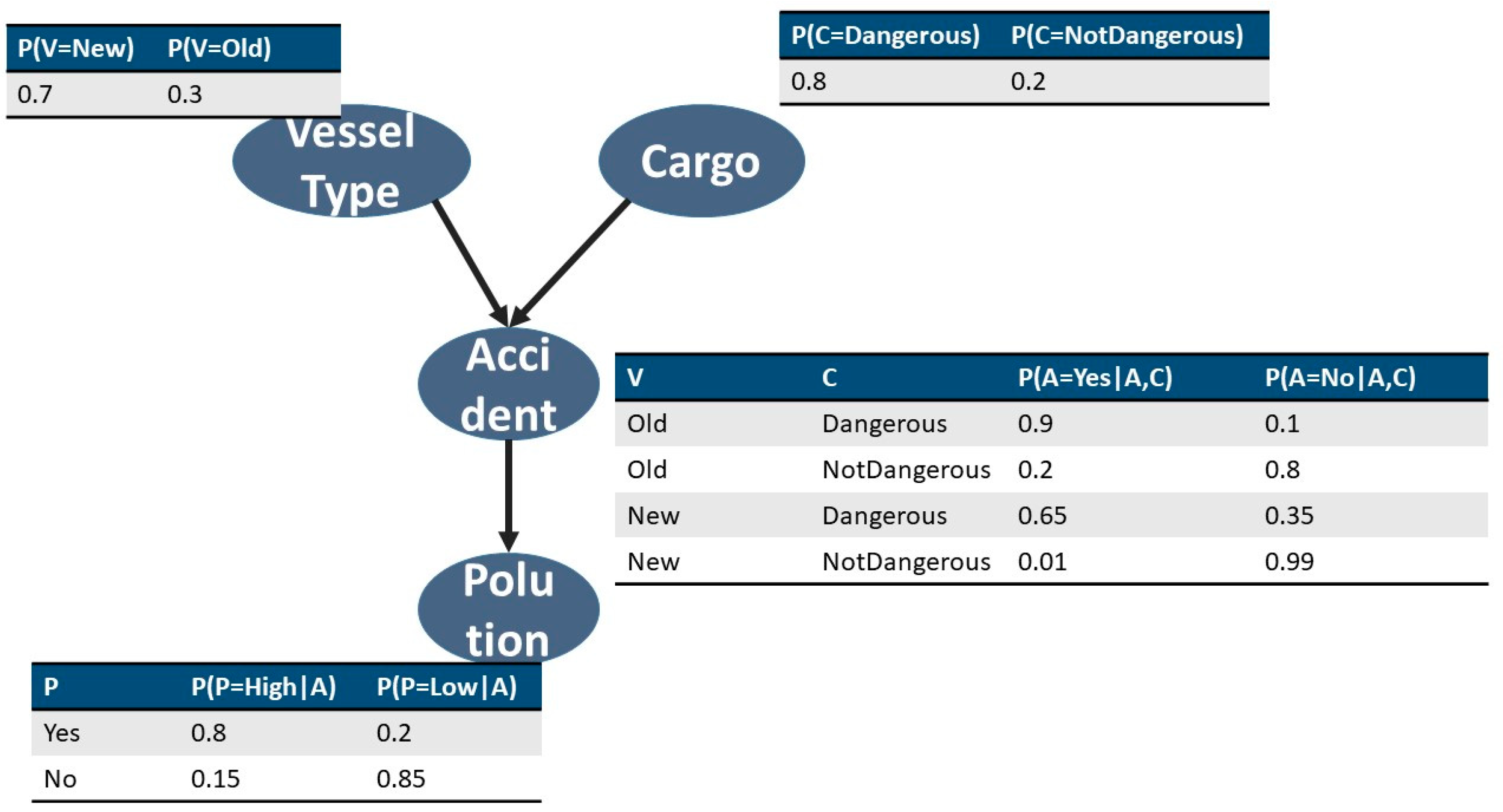
• The variables VesselType and Cargo are marginally independent, but when Accident is observed (given) they are conditionally dependent. The type of this relation is often named as explaining away.
• When Accident is given, Pollution is conditionally independent of its ancestors VesselType and Cargo.
• Instead of factorizing the joint distribution of all variables using the chain rule, such as P(V,C,A,P) = P(V)P(C|V)P(A|C,V)P(P|A,C,V) the BN defines a compact JPD in a factored form, such as P(V,C,A,P) = P(V)P(C)P(A|V,C)P(P|A). Note that the BN structure reduces the number of model parameters (i.e., the number of rows in the JPD table) from 2⁴ − 1 = 15 to only 8. This property is of major importance since it allows researchers to create a tractable model of domains with a plethora of attributes.

Such a reduction provides great benefits from inference, learning (parameter estimation), and computational perspective.

When people use BNs, they behave similarly to expert systems, since they allow representing beliefs and knowledge about a specific occurrence. The network represents the knowledge on a thematic area. Given evidence on the presence or absence of other situations, conclusions can be drawn on a particular situation. This important observation allows us to build information retrieval systems that are based on a straightforward probabilistic approach.

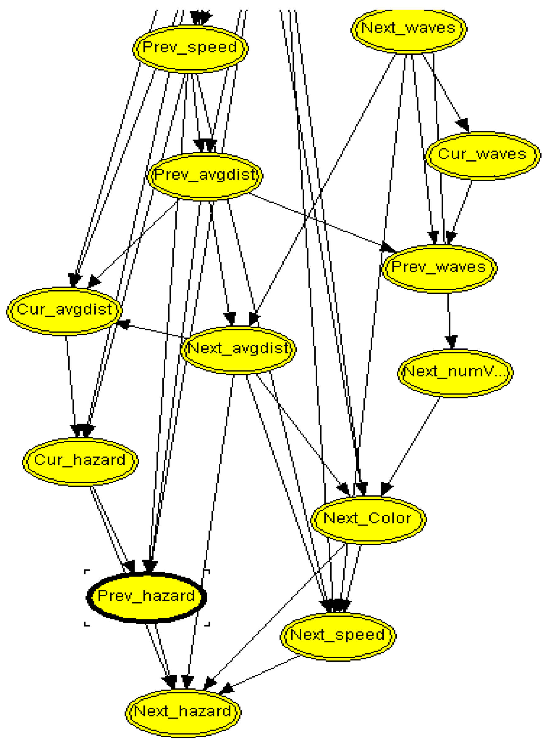
Hybrid Bayesian Networks

Managing BNs in domains where variables are continuous is not straightforward in a general way. The most common way to deal with the above situation is to discretize the variables and then use the known methods for discrete variables. Note however that this is an approximate approach, since we introduce some error in the discretization procedure.

There are some kinds of continuous variables in which the computations can be done in an exact way, one of which is the Multivariate Gaussian distribution. For the purposes of this study, a generalization of that model, the Conditional Gaussian (CG) distribution is adopted, in which discrete and continuous variables appear simultaneously, forming the so-called “Hybrid Bayesian Network” [20].

4. Marine Simulation System

The detailed description of the marine data simulation framework is described in the following text. As already mentioned in the introductory section, it is operating in a twofold manner, namely, a data preprocessing and transformation process and the main process of simulation using Bayesian networks and visualization using Social Network Analysis.

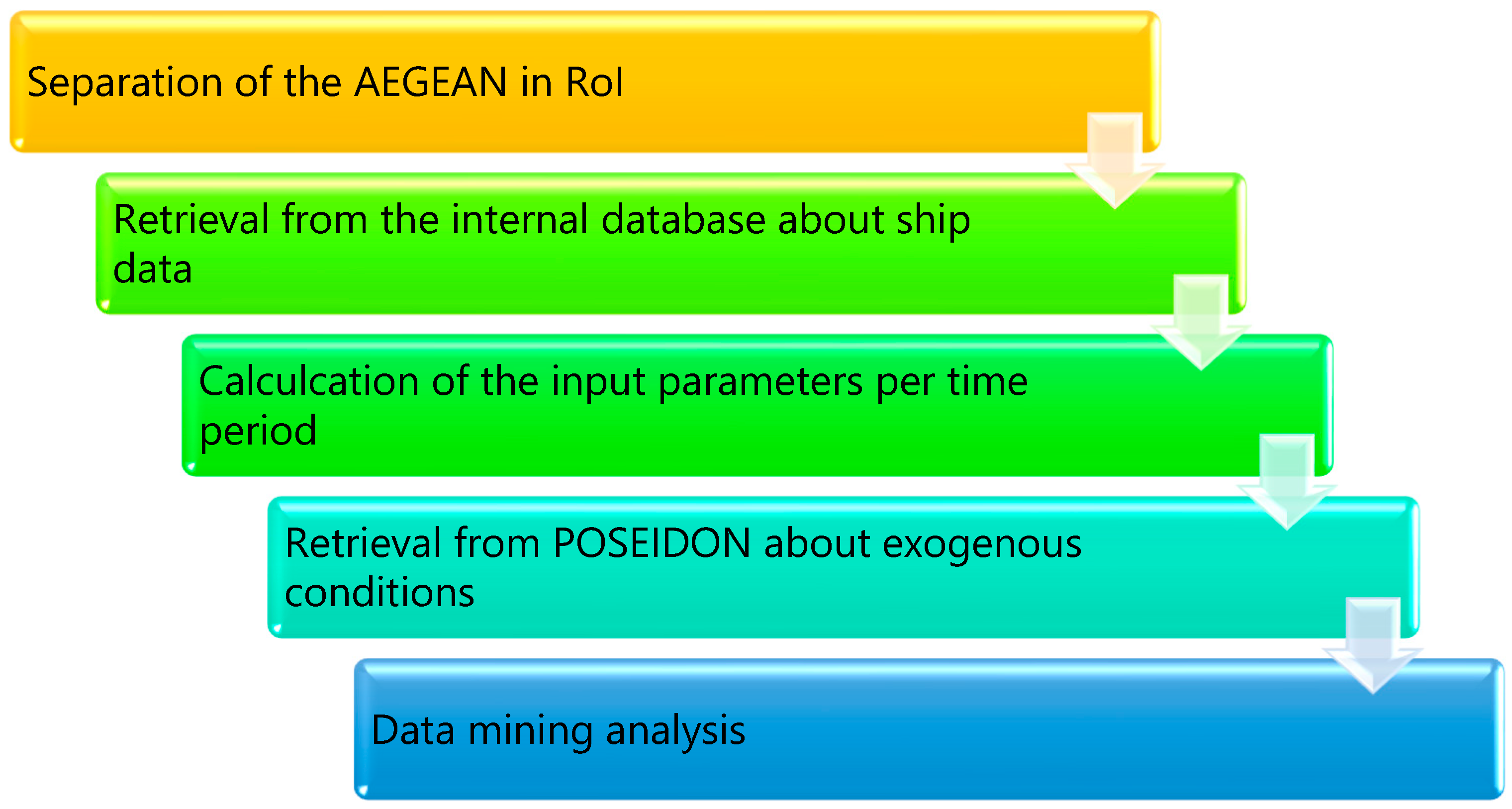
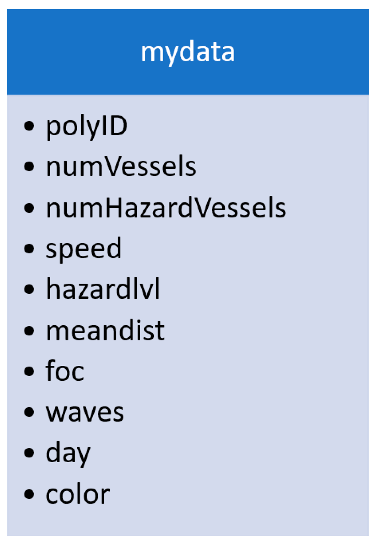
4.1. Data Description and Preprocessing

Figure 3 demonstrates the first phase of the data gathering approach. As one could observe from the above figure, the first operation is about constricting a spatio-temporal big data framework for building simulation processes on top of it. The current design supports the inclusion of a Region of Interest (RoI) that is adjustable is size, with granularity set to a value of about 38 km~1500 km² for our area of interest. Different levels of granularity were thoroughly evaluated and in spite of being supported, results have shown that low areas pose significant computational and managerial restrictions to the latter components of the system such as the data mining and the Bayesian network component without gaining significant forecasting outcomes.

The second step is the retrieval of static and dynamic ship data. More specifically, the location, the average speed in knots and the cargo, associated in a scale of A to D, with A considered the most hazardous. Additionally, data about sea conditions such as wave height was automatically retrieved by the POSEIDON system of the Hellenic Center of Marine Research (HCRM).

These features are used to construct the spatial objects. From such objects, input parameters needed by the simulator will be estimated. Such parameters include the number of ships found within a RoI, the average speed, the number of ships that carry hazardous load and the average distance between ships. As depicted in Figure 3, these parameters are aggregated per time period, from a day to a week and finally to a month. In order to represent data in a spatial dimension, the freely available Spheres library was used. Despite the fact that PostgreSQL provides methods for creating, indexing and querying spatial data, the Spheres library was preferred due to its programming properties and the simplicity in use.

The same approach is followed towards retrieval of exogenous conditions such as the sea wave-length. Such data are retrieved by the POSEIDON system, which is linked to our tool via RESTful interconnection. The preprocessing tool’s main task is to create a list of aggregated criteria per RoI, such as the number of ships, the average speed within this area, the density of the ships in the area and the sea conditions. The next phase focuses on applying clustering, an unsupervised data mining technique to these regions. Clustering organizes RoIs into groups of similar behavior, aiming at identifying in an unsupervised manner the hazardous and non-hazardous clusters.

Various clustering algorithms were examined and evaluated such as K-means, Expectation Maximization and DBSCAN. Upon completion of this unsupervised phase, statistical measures were extracted for each cluster and the danger level was assigned by a domain expert, resulting in a set of six dangers levels. More specifically, as mentioned in the Acknowledgements Section, the domain expert was the Hellenic Ports Association (ELIME), a collaborator of project AMINESS that funded this work. The method for assigning these levels was through survey forms to the members of the ELIME association. The process for allocating the optimal number of clusters is explained in the following section, namely Experimental Results. The exact methodology is depicted in Figure 4.

The last step of the data gathering approach is to update the internal database with information from the above process. In order to help users evaluate the outcome of this process, a graphical, web interface has been developed. The interaction course is depicted in the two figures below (Figure 5 and Figure 6):

On the left side of the page, the user can choose the criteria on which simulation will be based on. These criteria (they are shown in Greek in the portal) are:

• Number of ships

  ○

  It represents the total number of ships that passed through that RoI in a whole time slot (day, week, month)

• Average speed

  ○

  For each RoI, the speed of each instance is averaged on the number of instances

• Hazardous cargo

  ○

  the most frequent hazard level, as extracted by looking at all cargos from ships that passed through this RoI (i.e., nominal value from A to D, A denoting the most hazardous situation). This is a weighted value in order to give more emphasis on the hazardous load.

• Ship density

  ○

  The average distance between all ships that passed through a RoI.

• Wave height

  ○

  As retrieved from the POSEIDON system

Finally, there is another criterion which is not shown to the user but taken into consideration by our approach. This criterion is the number of ships with flag of convenience. Upon selecting the criteria and the time period, results of data mining are presented as shown below:

As depicted, RoIs are drawn using different coloring levels. A transparent RoI denotes safe areas while yellow to dark red represent increasing levels of danger. This information is also stored in the database for future use by the simulation component. From a technical point of view, this visualization interface utilizes Google Maps API and JavaScript (jQuery and jQuery UI).

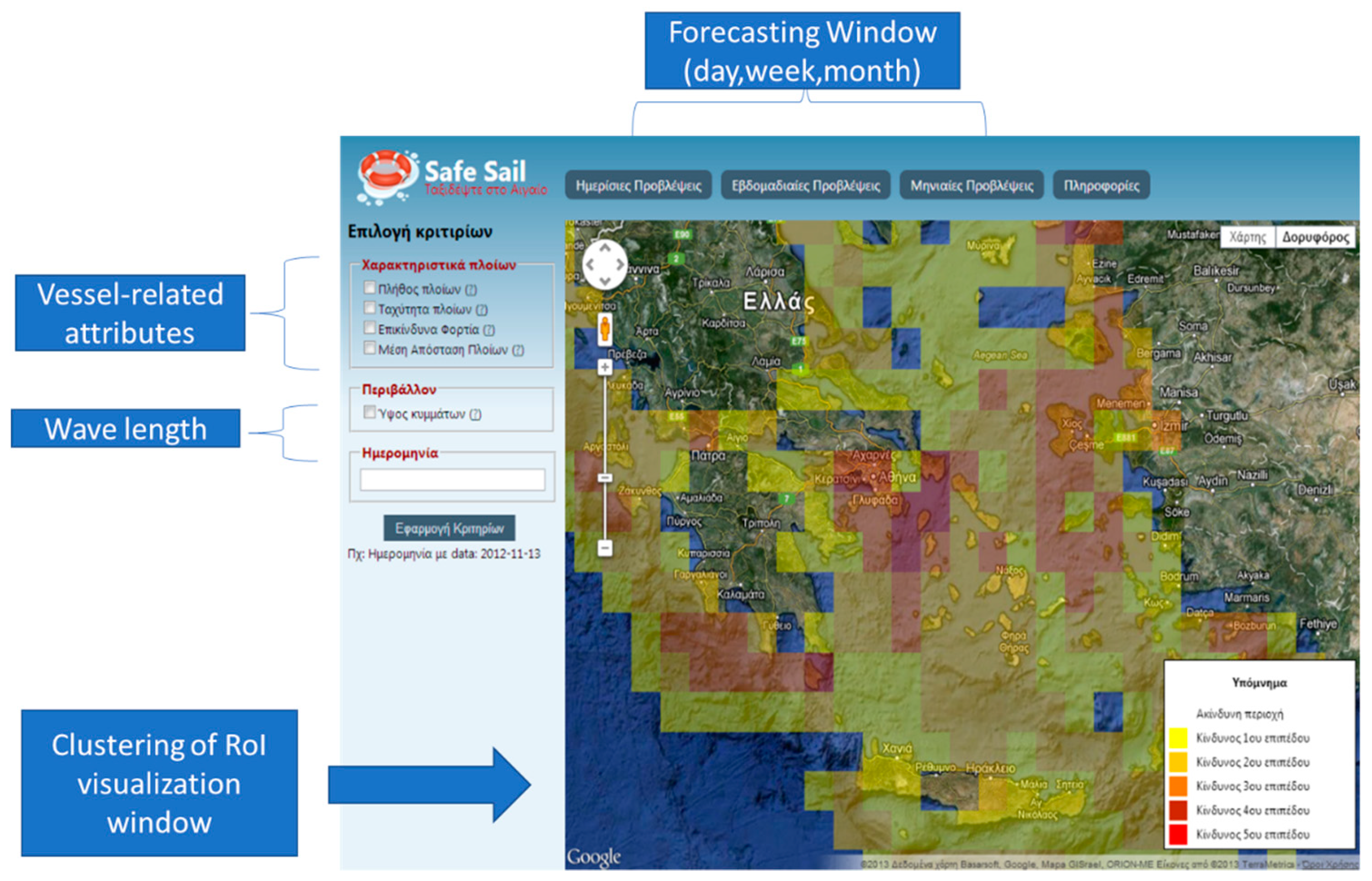
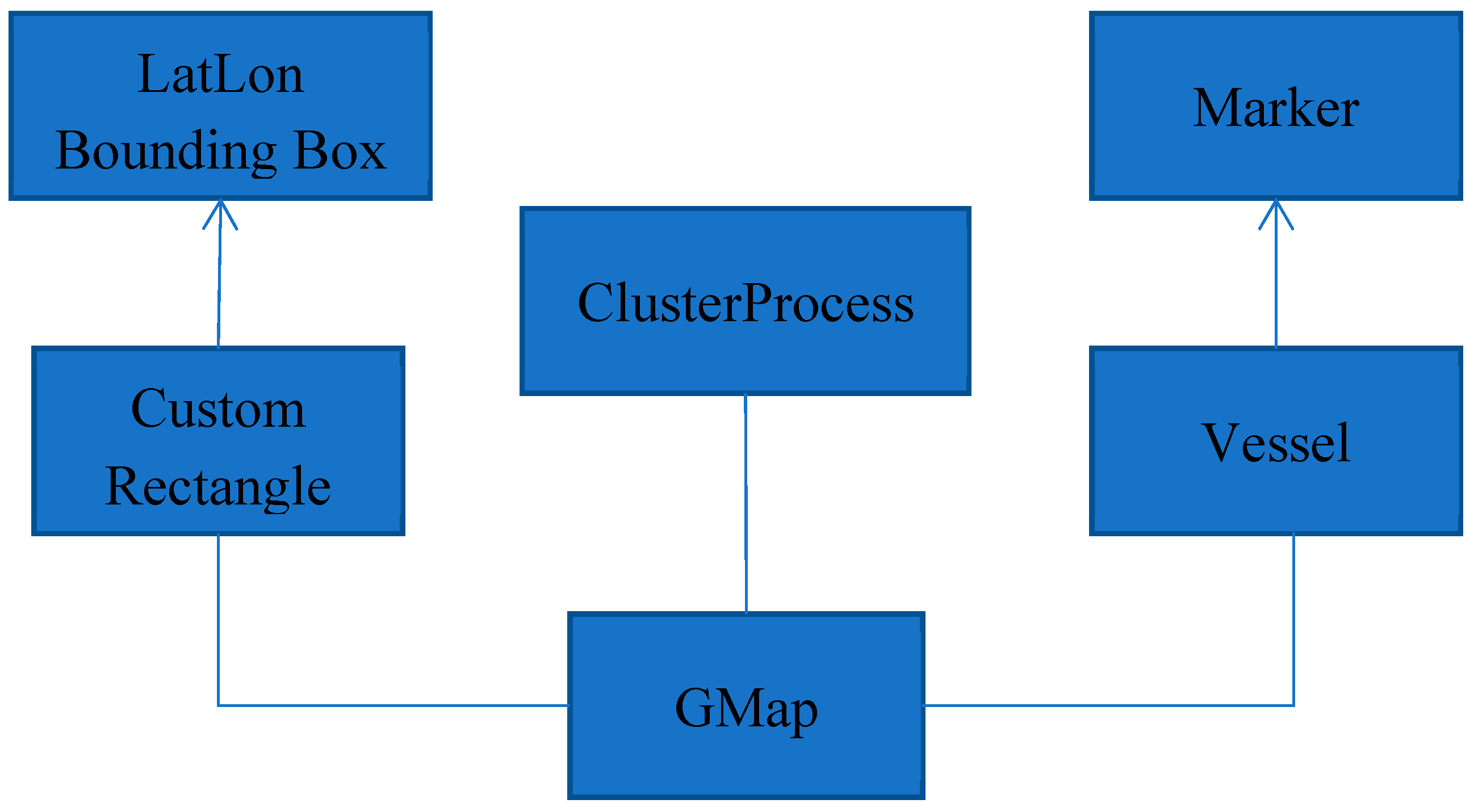
4.2. System Programming Details

The main database schema adopted is illustrated as Figure 7:

The first table contains the position, speed, orientation, status (such as anchored, cruising, etc.) and the time of message reception by the receiver. The second table refers to the ship’s static details and is connected to the dynamic data via the mmsi field. The static data are useful when extracting the flag of convenience, size, age, etc. Finally, the third table contains details on the type of the ship, and the hazard level of cargo. From this table, the preprocessing tools is creating the spatio-temporal data for the smallest granularity level, which is set to a day. The aggregated data are stored on the following database table as shown as Figure 8:

Each RoI is assigned a unique key (ID). All the other fields correspond to the criteria mentioned earlier. Finally, the outcome of the clustering process is coded as field color (numeric) on a scale from −1 to 5, −1 meaning no hazard and 5 meaning very dangerous area.

In order to record ship movements within an area, we split the AEGEAN area into spatial polygons and the application asks the database about passing ships, speed and hazard level. Since the RoI size is adjustable, data preprocessing from database would require numerous database I/O operation. Therefore, we have created a series of classes in Java that could help this process by performing a plethora of spatial operations in memory. Figure 9 shows these class connections.

The main class is called GMap. Its duty is to create a map and the separation into RoI, each one with the marine criteria. The separation of the map into regions is achieved by providing the top left point, the size of rectangles (squares) and the number of areas, horizontally and vertically. The predefined values are the separation start point, using Latitude 41.00000001 and Longitude 18.00000001 in order to cover the Hellenic Seas. Afterwards, the CustomRectangle class creates the remaining RoI, also calling the method for retrieving data from the database and preprocessing them to find the criteria. The CustomRectangle object extends the LatLonBoundingBox object, from the Spheres library, which provides a spatial polygon object. When reading data from database, GMap creates a connection and asks for ship information, creating a Vessel object along with all the ship’s characteristics. As described earlier, the connection closes and all spatial operations and queries are performed using the Spheres library. As soon as all vessels are identified (using the Marker object) in each RoI, the hazard criteria are calculated, as well as density. In order to retrieve the wave height from POSEIDON, the Gmap object is using a method (called waves) for asking a Live Access Server (LAS) using the center of each RoI as anaphora. The LAS usually responds as text and then the Gmaps object aggregates values from hours to per day granularity. Subsequently, the ClusterProcess method is called in order to cluster the created dataset. ClusterProcess can be called with different arguments as regards to the clustering method and its internal parameters. Finally, a reconnection to the database is performed in order to update clustering outcome (the danger level of each RoI) into table mydata (field color).

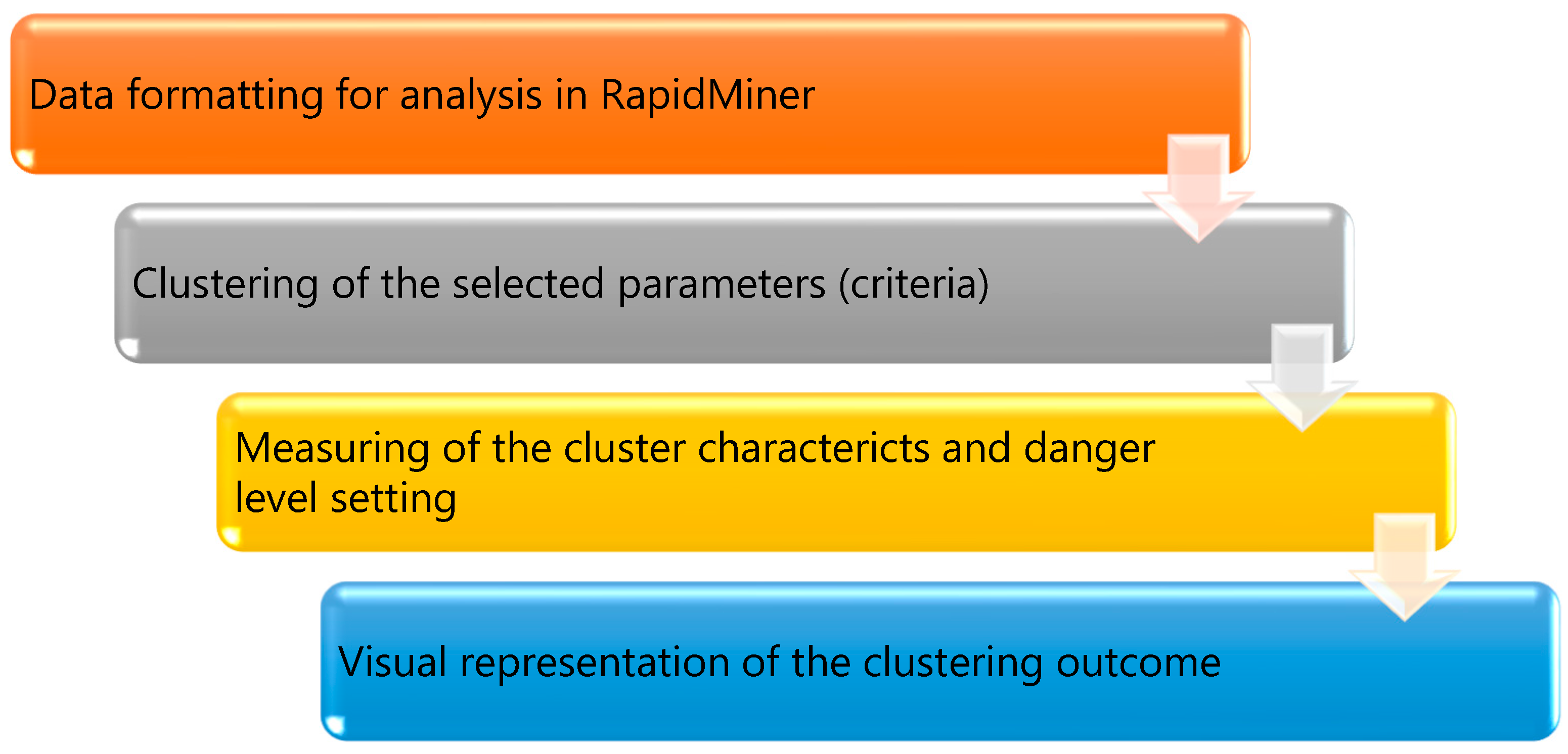
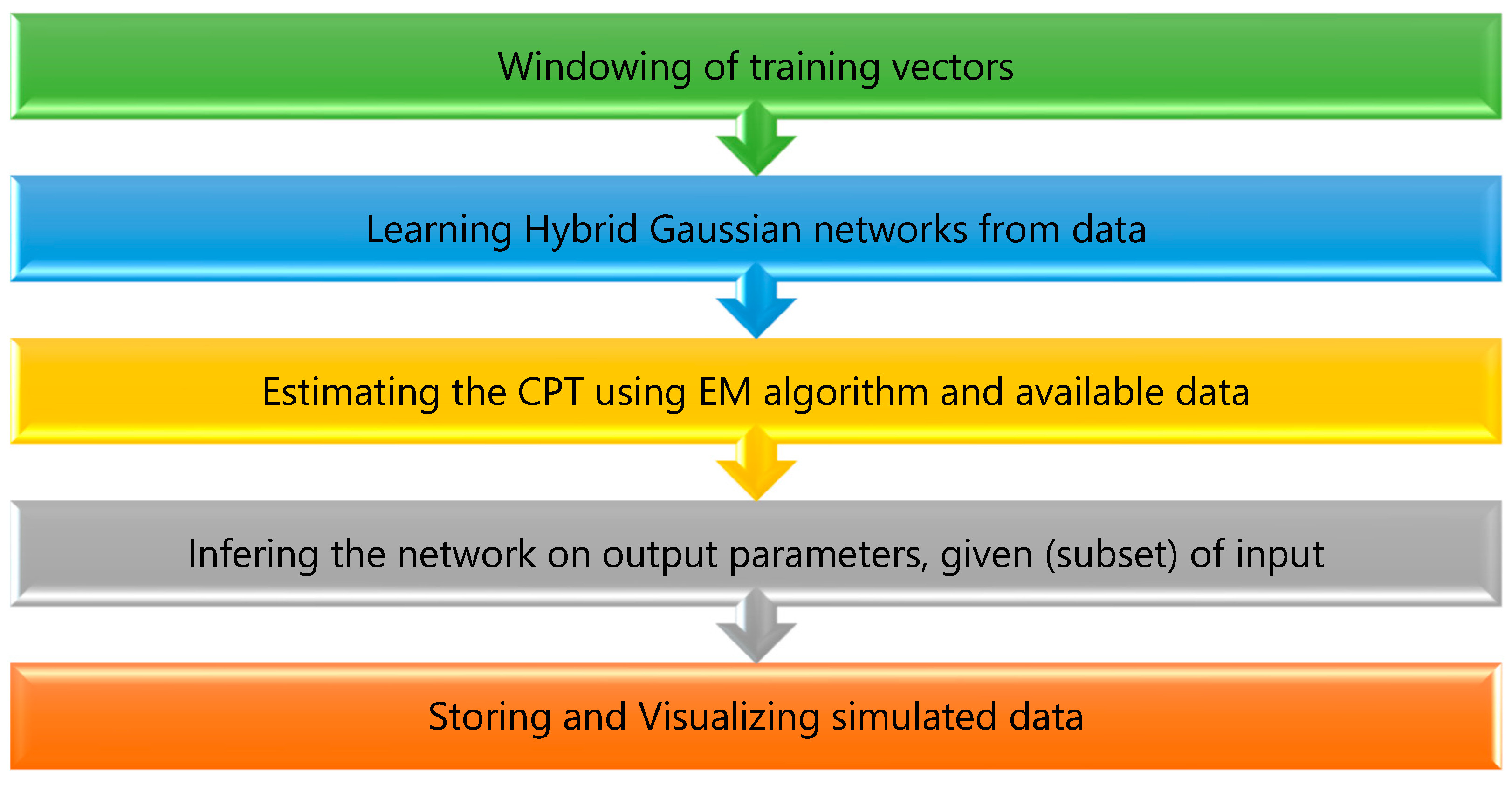
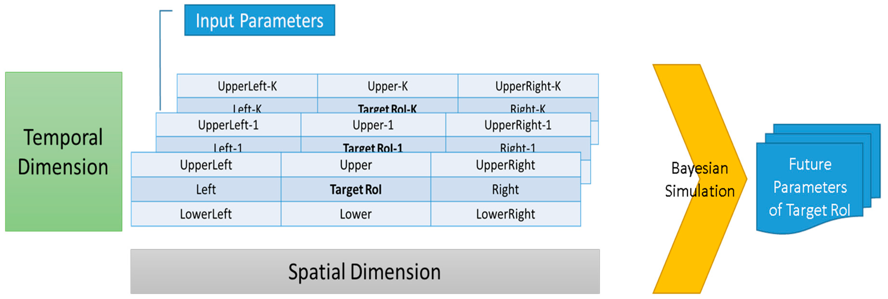
4.3. Simulation Phase

Figure 10 depicts the second stage of the proposed framework.

The first step prepares data for the simulation phase. We model the database instances as a multi-variate time series where geospatial information also contributes to the data. More specifically, for each RoI, the parameters presented above are windowed not only in time (e.g., the current period and the previous period) but also as regards to the neighboring conditions. As an example, consider Figure 11:

As it can be observed, for each RoI (called “target”), the set of its eight neighboring RoI is considered. Within each RoI, the set of input parameters is kept (as described in the previous subsections). This comprises the spatial dimension of the windowing process. As regards to the temporal dimension, we consider a varying window of K previous periods.

The second step is dealing with feeding the new, augmented vector to the Bayesian learning process. The learned structure is used later to estimate the Conditional Probability Table (CPT) of each node. The CPT is constructed using the Expectation Maximization algorithm along with observed data from the database. Figure 12 illustrates a small subset of the trained BN.

The training process is performed off-line. Upon learning of the structure and parameters (CPT) of the network, inference on the nodes which represent the future values, given the observed ones, is performed, in order to predict the future parameters of the target RoI, given the whole set or a subset of the available input parameters. Simulated data is then stored on a separate database, for exploitation and visualization purposes.

5. Experimental Evaluation

This section discusses the outcome of the experimental evaluation of the simulation tool. It is divided in two section, with the former focusing on the evaluation of the clustering procedure and the latter reporting the performance on Bayesian inference, the main mechanism we adopted for simulation.

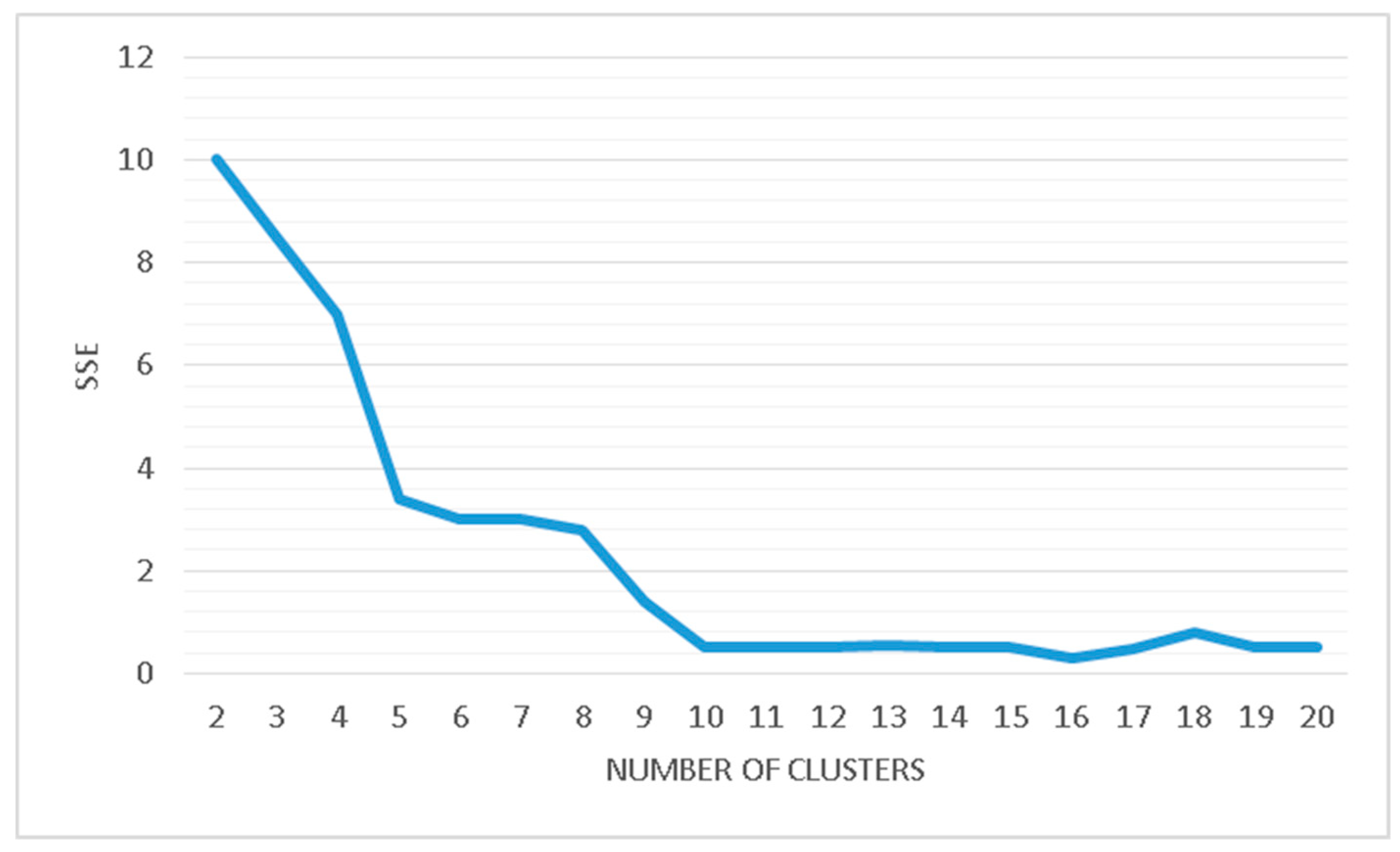
5.1. Measuring Clustering Validation

Clustering is used for the analysis of data because knowing how many and which of the areas are dangerous in advance is not feasible. Moreover, allowing for human intervention for the classification of danger in each area is not practical due to the tremendous laboring effort it would require. It is the task of clustering to organize a set of objects in such a way that objects in the same group (called a cluster) are more similar to each other than to those in other groups.

In order to find the most appropriate clustering method, three well known and theoretically different algorithms were benchmarked, such as k-Means [21], Expectation Maximization (EM) [22] and DBSCAN [23]. The first algorithm is based on clustering by using the most representative object of a cluster, that is a centroid, the second algorithm uses data distributions in an iterative manner for the separation of clusters, while the latter makes use of the density of the data set. In density-based clustering, clusters are defined as areas of higher density than the remainder of the data set. Objects in these sparse areas - that are required to separate clusters - are usually considered to be noise.

The first issue we had to deal with is the optimal number of clusters to be concerned. In solutions such as K-means and EM, this parameter is needed as input. A good way to find that number, is to consider various values and then for each clustering solution returned by each algorithm to estimate the sum of squared error (SSE), given by the following formula:

$$SSE={\displaystyle \sum }_{i=1}^k{{\displaystyle \sum }}_{x\in C_i}dist{\left(c_i,x\right)}^2$$

where C_i is the i-th cluster and c_i (in lower case) represents the centroid of C_i.

By plotting the SSE of the k-Means algorithm against different values for k (k = number of clusters to be found) the optimal k lies at the point where the curve makes an immediate slope. As one could notice by examining Figure 13, this phenomenon occurred for k = 10, therefore this was the initial solution. However, when discussing with two domain experts from the Greek Ports Association, it was decided that this should change to a lower value, since having so many danger level intervals is not user-friendly, especially at the visualization phase. Similar behavior was observed for the EM as well.

Given that the ground truth labels are not known, evaluation must be performed using the model itself. The criteria for comparing the results of all three algorithms are the density of each cluster and the Silhouette Coefficient [24,25]. For density, the Euclidean distance was used as distance metric. The lower the value of density is, the more similar the components to each other are and thus, the more compact a cluster is.

$$Performan{e}_{o{f}_{clustering}}=\frac{{{\displaystyle \sum }}_{j=1}^n\sqrt{{{\displaystyle \sum }}_{i=1}^m{p}_{j{a}_i}-p_{{\left(j+1\right)}_{ai}}}}{n\ast \left(n-1\right)}$$

where n denotes the number of points of a dataset, m is the number of clusters and $p_{j{a}_i}$ is a specific point j from the total points n belonging to a given cluster αi from the total number of clusters m.

According to the above formula, the Euclidean distance is calculated between points using all of their features and the average of all of distances is returned. Afterwards, it is multiplied by the number of elements of the cluster minus one and the resulting number represents the performance of each clustering method.

To calculate the total performance of an algorithm the performance of each cluster is summed by weighting the number of components that are contained in each cluster and divided by the total number of components.

$$Total\_Performance=\frac{{{\displaystyle \sum }}_{i=1}^{n}Performane\_of\_cluste{r}_i\ast components\_of\_cluste{r}_i}{total\_number\_of\_components}$$

As regards to the latter performance metric, a higher Silhouette Coefficient score relates to a model with better-defined clusters. The Silhouette Coefficient is defined for each sample and is composed of two scores:

a: The mean distance between a sample and all other points in the same class.

b: The mean distance between a sample and all other points in the next nearest cluster.

The Silhouette Coefficient s for a single sample is then given as:

$$SC=\frac{b-a}{max\left(a,b\right)}$$

Three different time periods were chosen randomly, namely day, week and month. The total number of RoI for the Aegean Sea was 672, given the square size of 1 km per side. Each algorithm was tested based on predefined chosen criteria, except (a) the number of k, in k-means and in EM algorithms k was chosen to equal to 6 and (b) in DBSCAN algorithm the variable ε is replaced by a value of 1.0 and the min_points was set to 5. Parameter ε specifies how close points should be to each other to be considered as part of a cluster and parameter min_points specifies how many neighbors a point should have to be included into a cluster. Since the choice of such parameters plays a crucial role in the validity of clusters, we followed estimated the distance from each point to its nearest neighbor and created a histogram. By examining the value of distance units where the vast majority of points lie within provides a good estimate of the ε parameter. Consequently, for that ε value, we examined how many points lie within each point’s ε-neighborhood. Again, by visually examining the histogram, we exclude the values that have too few neighbors and look for values that start having an increasing number of neighbors. Parameter min_points is chosen as the value where the number of neighbors begins to grow.

According to literature, the most efficient algorithm (with the best performance) is the one with the smallest absolute value of density. By executing the evaluation process, the following results were returned, tabulated on

Table 1. Cluster Density evaluation results upon the selected clustering algorithms.

	k-Means	DBSCAN	ΕΜ
Day	−748.720	−3582.824	−1705.336
Week	−769.273	−3701.001	−1715.009
Month	−991.182	−3717.501	−2195.938

, referring to cluster density while

Table 2. Silhouette Coefficient evaluation results upon the selected clustering algorithms.

	k-Means	DBSCAN	ΕΜ
Day	0.741	0.343	0.610
Week	0.733	0.311	0.606
Month	0.681	0.303	0.588

tabulates the Silhouette Coefficient score for the same experimental setting:

According to the results of Table 1, it is apparent that the algorithm with the lower average density and with almost threefold difference in clustering is the k-Means. The same trend appears on the second table as well, denoting that k-Means is the most accurate clustering model.

In addition, the speed of execution of the k-Means algorithm is slightly faster of this of DBSCAN, while the EM algorithm runs more slowly. Measurements were made on a sample of three different time periods, taking into consideration all the criteria of data analysis. Additional parameters of k-Means or differentiation of k extract values quite close to those of k = 6 and we considered using more clusters for the evaluation of the sample as unnecessary.

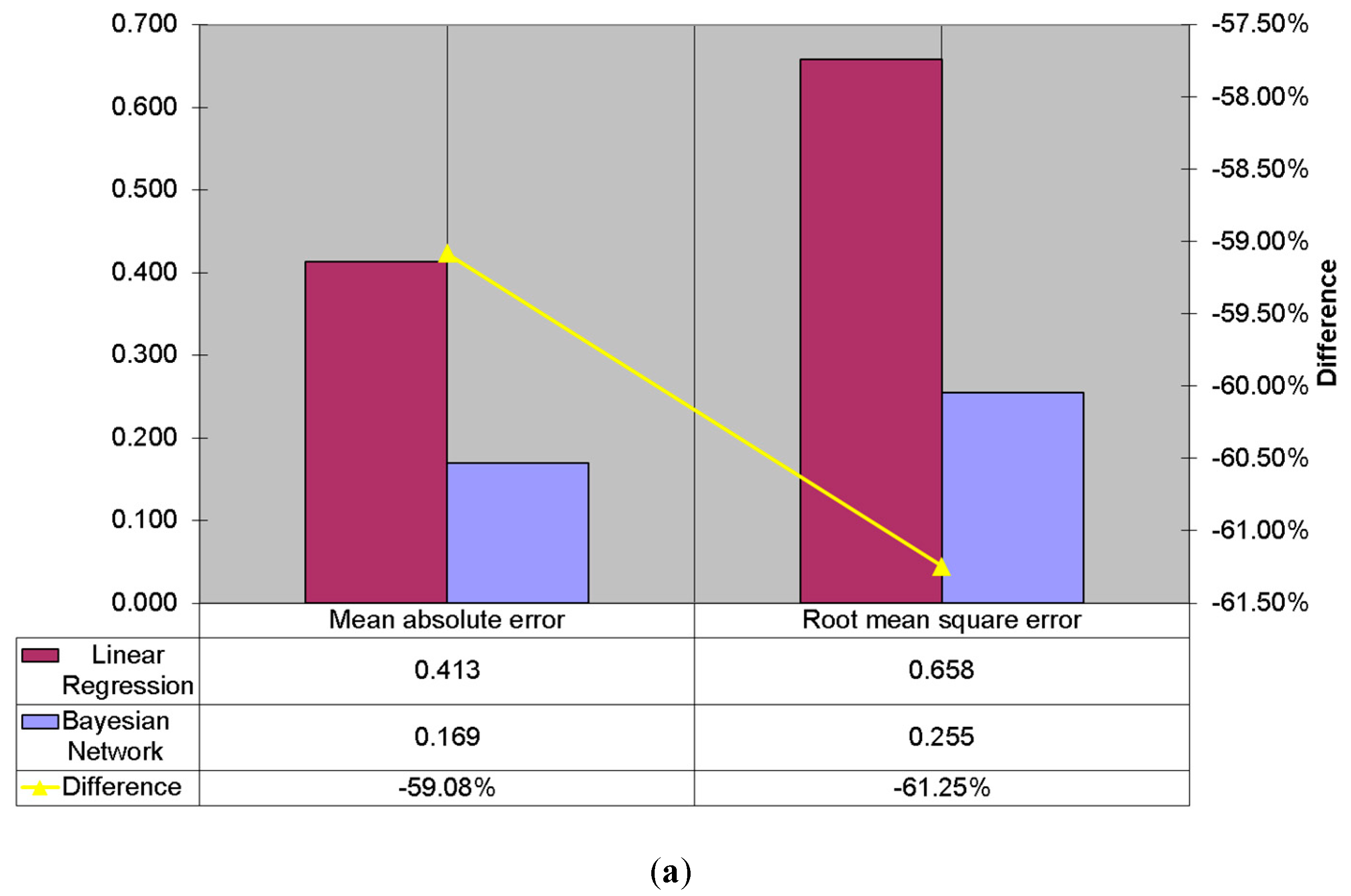
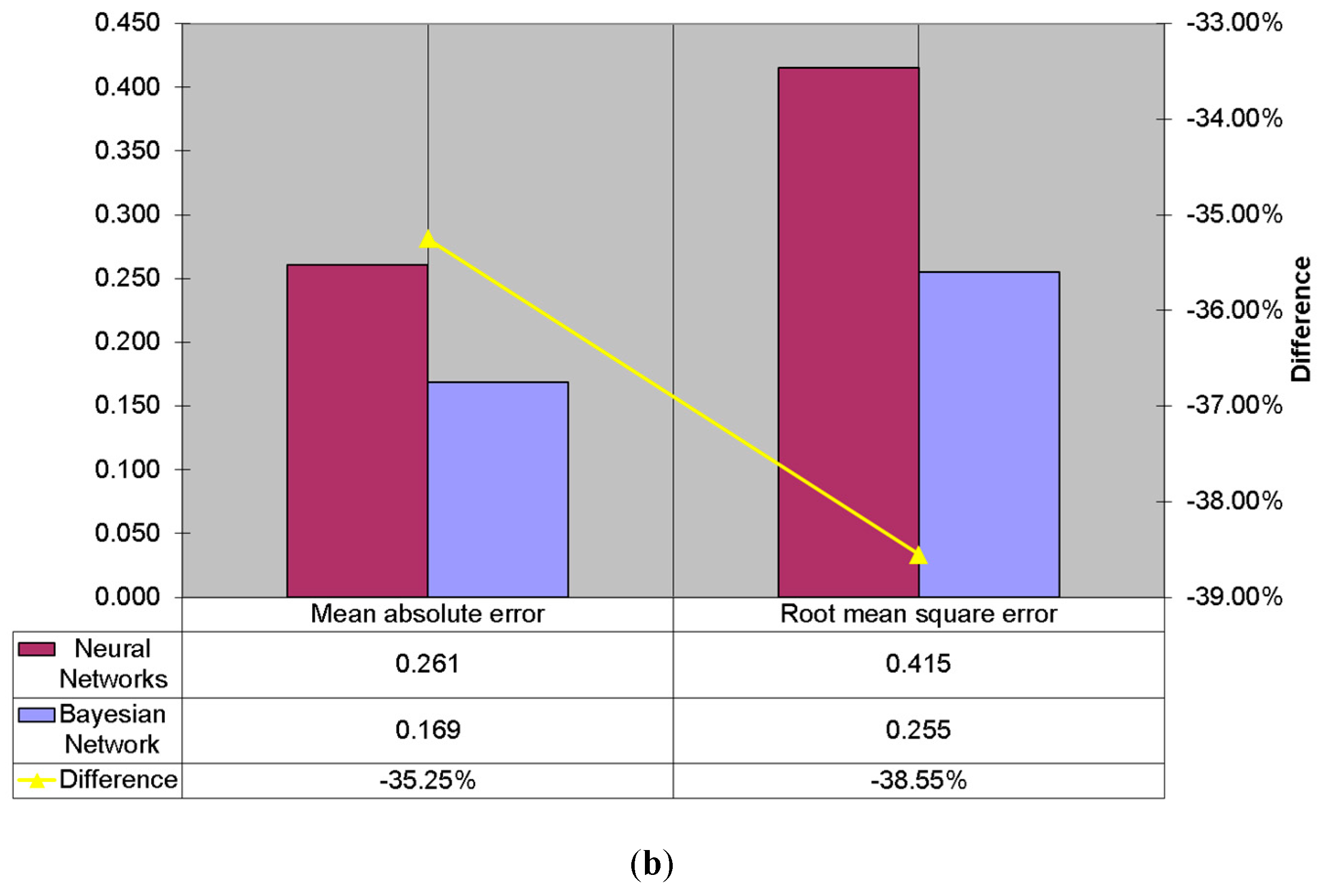
5.2. Evaluation of the Inference Performance

In this experimental setting, we are mostly interested in measuring the inference ability of the hybrid Bayesian network in one selected output parameter, namely danger level. Certainly, the network is able to simultaneously forecast the future values for all output parameters, but for reasons of readability, the aforesaid was selected. Since the majority of similar works utilize linear regression analysis and neural networks, a benchmark of the performance of the proposed method is provided against Linear Regression and Multi-layer perceptron Neural networks (NN). The method of 10-fold cross validation was used, in which the dataset is iteratively partitioned into two distinct subsets, a train and a test set, using a 9:1 ratio. Algorithms are trained using the former set and their forecasting models are tested on the latter. This step is repeated 10 times using different train and test subsets. The result is the average performance over the 10 experimental runs. About performance evaluation, the following metrics were used:

5.2.1. Mean Absolute Error

The MAE E_i of an algorithm I is calculated by the equation:

$$E_i=\frac{1}{n}{\displaystyle \sum _{j=1}^n\left|P_{(ij)}-T_j\right|}$$

where P_(ij) is the value that algorithm I forecasted for a j-th sample (from a set of n examples) and T_j is the value of the ‘target value’ for the j-th example. For an ideal classification, P_(ij)= T_j and E_i = 0. So, the E_i indicator varies from 0 to infinity, with 0 to correspond to the ideal classification.

5.2.2. Root Mean Squared Error

The RMSE E_i of an algorithm I is calculated by the equation:

$$E_i=\sqrt{\frac{1}{n}}{\displaystyle \sum _{j=1}^n{\left(P_{(ij)}-T_j\right)}^2}$$

where P_(ij) is the value that algorithm I forecasted for the sample j (from a set of examples) and Tj is the value of the ‘target value’ for the j-th example. For an ideal classification, P_(ij) = T_j and E_i = 0.

Figure 14 shows the forecasting performance of the three algorithms, namely the hybrid Bayesian network, Linear Regression and Neural Networks, depicted in pairs of two (our method against each other approach suggested by literature).

As seen above, the adopted solution outperforms Linear Regression in both error rates by more than 60%, supporting our claim that Bayesian analysis is well suited for the task at hand, providing also semantic interpretation of the variable relations. The same applies at the comparison with NN, where again, the Bayesian network performs better, portraying an error rate approximately 35% lower than that of NN.

Despite the fact that the obvious approach when comparing two forecasting models is to select the one that has the smaller error measurement based on one of the error measurements described above, we have to decide if this difference is significant or basically due to the specific choice of data values in the sample. Hence, each of the three forecasting models, namely Linear Regression (LR), Bayesian Networks (BN) and Neural Networks (NN), was compared to the others in terms of the Diebold-Mariano (DM) test [26]. Taking the null hypothesis: “both forecasting models have the same accuracy” into consideration, the DM test returns two measurements, that is a p-value, denoting that the hypothesis holds when close to 1 or does not hold when close to 0 and DM-statistics, measuring the squared errors of the two models. Negative values show that the squared errors of the model listed first are lower than those of the model listed last.

Table 3. DM-test results for all forecasting models, carried out in pairs.

Null Hypothesis: Both Forecasts Have the Same Accuracy
p-value	LR	BN	NN
LR		0.0073	0.6311
BN			0.0088
NN
DM statistic	LR	BN	NN
LR		0.6264	0.4305
BN			−3.8733
NN

tabulates the DM-test outcome between all forecasting models. By examining the p-values of pairs LR-BN and BN-NN we can observe that they are very close to zero (i.e., 0.0073 and 0.0088 respectively) denoting that the null hypothesis that both models have the same accuracy is not statistically valid. Considering the last pair between LR and NN we can clearly observe that their p-value is significantly larger than 0. The same conclusion could be drawn by examining the DM-statistic metric. Again, it is observed that BN have significantly lower error rates than the other two models.

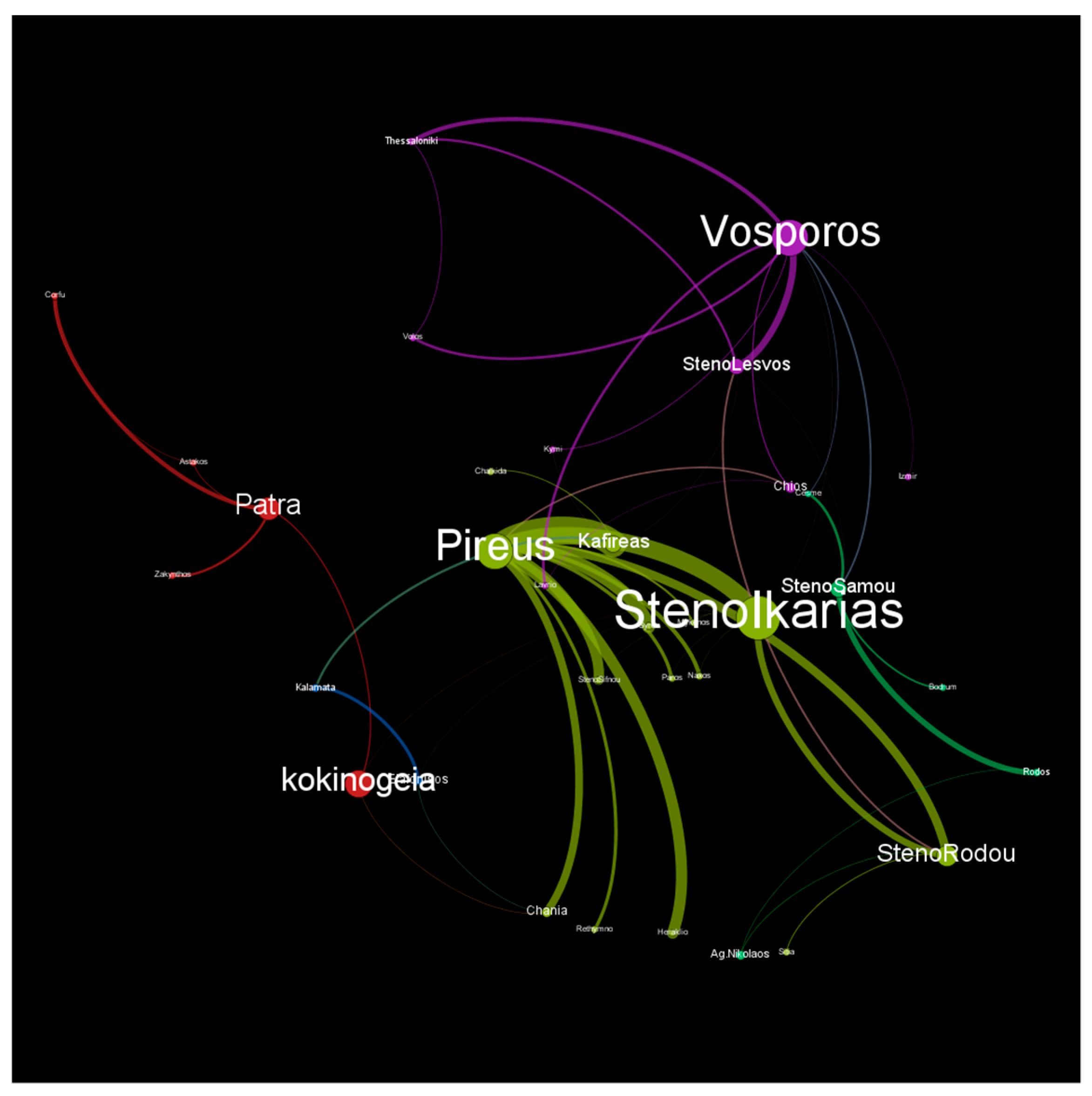
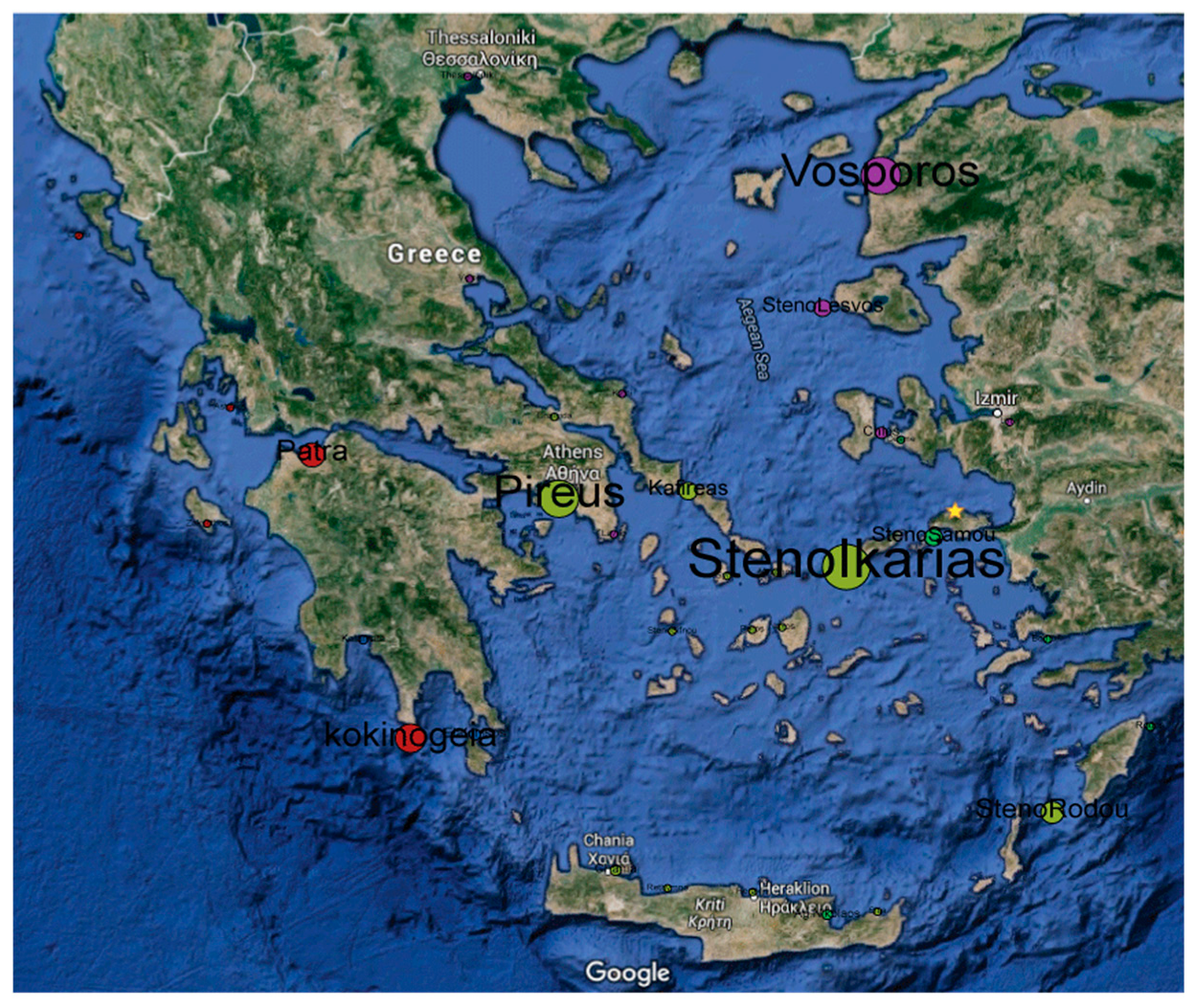
6. Modeling Marine Transportation as Social Network

Upon simulation, we aimed at extending the framework to support more advanced visualizations functionalities. Thus, we borrowed techniques from the area of Social Network Analysis (SNA). We model the ship traffic domain as an undirected network, whose nodes correspond to selected RoIs that need special attention (such as ports, regions that are beings crossed by major passaging vessels) and arcs represent the trajectories of vessels moving from one node to another. The network would be then analyzed by using conventional SNA analysis algorithms and visualized in constant time or in discrete timeslots, in order for domain and policy experts to observe dynamic changes over time. The idea is that transportation of ships may be considered as a form of social network where nodes represent points in the sea where significant traffic is being observed and arcs can be considered as preferences of ships over moving across specific points. In an attempt to model maritime flow, we should take the fact that a maritime network is an assemblage of individual vessel trajectories that are subjected to spatial constraints. Therefore, by analyzing such networks we could identify influential points that could potentially become areas of high risk in terms of accidents, touristic development, port authority strategic planning, etc.

More specifically, historical AIS data were transformed into trajectories using the original geolocation information and applying a linear interpolation model. Upon trajectory construction, the network’s nodes were divided into two categories, namely static (ports) and dynamic (areas where several trajectories of ships cross). The arcs corresponded to the passing of ships from one node to another, again based on their extracted trajectories (usually weighted by some criterion, such as average speed or average number of ships). The quality of this network was measured, utilizing metrics such as centrality, density, modularity, PageRank score, etc.

Using the Java language and the freely available Gephi® library, visualization could take place, either in a static time period or in a sliding window of time.

6.1. Social Network Analysis Measures

The present section illustrates the various metrics that can be encountered during a network analysis phase, in order to understand the underlying concepts and relations. The five most significant concepts that are commonly used in social network analysis tasks are closeness, network density, centrality, betweenness and centralization. In addition to the aforementioned, there are four other measures of network performance that include: robustness, efficiency, effectiveness and diversity. The first set of measures deal with the structure of the network while the second set of metrics focuses on the dynamics and thus depend on a theory explaining why certain agents do certain things in order to access the information [27].

Closeness reflects the ability to access information through network members. Network density is a measure of how connected a network is. Node centrality denotes the number of ties with other nodes while betweenness of a node measures the extent to which an agent (represented by a node) can play the part of a broker or gatekeeper with a potential for control over others. Centralization provides a measure of the extent to which a whole network has a centralized structure.

Robustness can be evaluated based on how it becomes fragmented when an increasing fraction of nodes is removed, whereas network efficiency can be measured by considering the number of nodes that can instantly access a large number of different nodes. Effectiveness targets the cluster of nodes that can be reached through non-redundant contacts and finally, diversity, conversely suggests a critical performance point of view where nodes are diverse in nature, that is the history of each individual node within the network is important.

6.2. Applying SNA to Marine Traffic Data

As previously described, all nodes were coded using the name of the port (in case of static nodes) and the name of the closest island or inland point for the dynamic nodes. In all cases, the latitude and longitude values were obtained. The network was formed by the aforementioned nodes and edges were placed by monitoring the ship movement over time. More specifically, when a ship was passing from a specific node a trigger was initiated that was alert until the ship passed from another node in the network for a given period and if not, the trigger was set to the initial value. For example, when a ship was found initially in the node that corresponds to the port of Piraeus, a trigger was initialized, waiting for the ship to enter another node in the network during a manually predefined period. In case it did, the counter of ships form Piraeus to the other node was increased by one and at the end of the day, if these counts exceeded a threshold value, an edge was established. From a technology perspective, the trigger was implemented using Oracle database triggers in PL/SQL language. The triggers were fired during INSERT/UPDATE operation within the framework’s database.

Figure 15 portrays a visualization based on the authority level of nodes, for the area of the Aegean Sea, followed by the same network layered on a map in order to clearly depict the areas of interest, see Figure 16. As we can observe, node colors correspond to the modularity class of the network, that is the different node communities that are formed, while network sizes reflect the closeness centrality. The label size is also proportional to this metric, helping visualization of the status of ship movements between these points of interests (i.e., nodes). The edges are weighed according to the number of ships moving between two nodes. Note that these edges could be weighted with other metrics such as average speed, type of cargo, weather conditions, etc., since all of the above are available from our database.

This figure can reveal and visualize important knowledge to domain experts from the AIS data. For instance, the green arcs portray significant marine traffic within the island group of Cyclades, and the island of Crete, some of the most touristic parts of Greece. Since there are both commercial and passenger ships that form the network, domain experts could examine imposing regulated waterways to the former since the effects of a potential accident including vessels with dangerous cargo would have catastrophic consequences for the economy and the environment.

In the figure below, the same graph as above is simplified by removing the edges and mapped onto a Google Maps’ layer of the Aegean Sea.

7. Conclusions

Marine traffic in the Aegean Sea has dramatically increased throughout recent years, mainly due to the need for marine transportation of fuels, materials and goods to and from the Middle East countries and the development of commercial agreements with Chinese factories and logistics. The increase in maritime traffic, despite the commercial benefits to the region, is posing significant challenges to the preservation of the local ecosystem and safety as well. This danger is further deteriorated from lack of regulations and unregulated waterways. Marine accidents may cause major ecological disasters and have socio-economic impacts in Greece. Monitoring the marine data is of major importance and one of the primary goals of the current research.

Real-time monitoring and alerting can be extremely useful to local authorities, companies, NGO’s and the public in general. Apart from real-time applications, the discovery of hidden patterns and trends is also significant. Towards this direction, a simulation tool for marine data has been designed and developed.

Recent advances in data storage and management as well as the great progress on data analytics methods have enabled Big Data analytics by researchers and developers. Based on free and commercial solutions, nowadays, an analyst could create advanced applications using minimal effort. Existing and newly developed solutions have been incorporated in order to create a framework.

The framework analyses historical data about ships and area conditions, of varying time and space granularity, measures critical parameters that could influence the hazard of a specific region and clusters such data according to their similarity. This process covers research question no. 1, namely the incorporation of various heterogeneous maritime and weather data towards identifying hazardous conditions. Upon this unsupervised step, the degree of hazard is estimated and along with the other parameters is fed into a special type of Bayesian networks [28,29], in order to infer on future situations, thus, simulating future data based on past conditions and addressing the related research question no. 2. The use of such a system is particularly beneficial for multiple stakeholders, such as the port authorities, the ministry of Mercantile Marine, etc. mainly due to the fact that specific policy options can be evaluated and re-designed based on feedback from our framework. Finally, maritime flow has been modeled and analyzed as a social network to address the third research question, which is the creation of useful visualization and insights for the domain.

Experimental results have portrayed that the suggested technique is more beneficial than other methods, such as neural nets and linear models for a variety of reasons, ranging from accuracy to computational issues. The tool is customizable in the sense that new criteria could be added, new danger estimation functions could also be supported and clustering could only be serving as a data organization method. In order to stress the practical applicability of the proposed study, the simulation framework could serve as an analysis and risk assessment tool as well as a decision support system for policy-making process by local authorities and domain experts.

References

1. Guziewicz, G.; Ślączka, W. Methods for determining the maneuvering area of the vessel used in navigating simulation studies. In Proceedings of the VII MTE Conference, Szczecin, Poland, 1997. [Google Scholar]
2. Papanikolaou, A.; Boulougouris, E.; Sklavenitis, A. The sinking of the Ro-Ro passenger ferry SS Heraklion. Int. Shipbuild. Prog. 2014, 61, 81–102. [Google Scholar] [CrossRef]
3. MaritimeCyprus. Available online: https://maritimecyprus.com/2018/12/11/ireland-ro-ro-passenger-ferry-epsilon-8-feb-2016-incident-investigation-report/ (accessed on 18 January 2019).
4. Kum, S.; Sahin, B. A root cause analysis for Arctic Marine accidents from 1993 to 2011. Saf. Sci. 2015, 74, 206–220. [Google Scholar] [CrossRef]
5. Kiousis, G. Γιώργος Κιούσης, Ζητείται... τροχονόμος και για το Aιγαίο. Ελευθεροτυπία, X.K. Τεγόπουλος Εκδόσεις A.Ε. Available online: http://www.enet.gr/?i=news.el.article&id=135365 (accessed on 18 January 2019). (In Greek).
6. Vafeiadis, N. Νίκος Βαφειάδης. Μια νάρκη στο βυθό της Σαντορίνης (SEA DIAMOND). Περιοδικό «Κ», τεύχος 236, σελ. 62-71. Available online: http://eyploia.epyna.eu/modules.php?name=News&file=article&sid=1454 (accessed on 18 January 2019). (In Greek).
7. Aarsæther, G.; Moan, T. Estimating Navigation Patterns from AIS. J. Navig. 2009, 62, 587–607. [Google Scholar] [CrossRef]
8. Chen, J.; Lu, F.; Peng, G. A quantitative approach for delineating principal fairways of ship passages through a strait. Ocean Eng. 2015, 103, 188–197. [Google Scholar] [CrossRef] [Green Version]
9. Shelmerdine, R.L. Teasing out the detail: How our understanding of marine AIS data can better inform industries, developments, and planning. Mar. Policy 2015, 54, 17–25. [Google Scholar] [CrossRef]
10. Tsou, M.-C. Online analysis process on Automatic Identification System data warehouse for application in vessel traffic service. Proc. Inst. Mech. Eng. M J. Eng. Marit. Environ. 2016, 230, 199–215. [Google Scholar] [CrossRef]
11. Fournier, M.; Hilliard, R.C.; Rezaee, S.; Pelot, R. Past, present, and future of the satellite-based automatic identification system: Areas of applications (2004–2016). WMU J. Marit. Aff. 2018, 17, 1–35. [Google Scholar] [CrossRef]
12. Goerlandt, F.; Goite, H.; Valdez Banda, O.A.; Höglund, A.; Ahonen-Rainio, P.; Lensu, M. An analysis of wintertime navigational accidents in the Northern Baltic Sea. Saf. Sci. 2017, 92, 66–84. [Google Scholar] [CrossRef] [Green Version]
13. Rezaee, S.; Pelot, R.; Ghasemi, A. The effect of extreme weather conditions on commercial fishing activities and vessel incidents in Atlantic Canada. Ocean Coast. Manag. 2016, 130, 115–127. [Google Scholar] [CrossRef]
14. Montewka, J.; Krata, P.; Goerlandt, F.; Mazaheri, A.; Kujala, P. Marine traffic risk modelling an innovative approach and a case study. Proc. Inst. Mech. Eng. O J. Risk Reliab. 2011, 225, 307–322. [Google Scholar] [CrossRef]
15. Almaz, O.A.; Altiok, T. Simulation modeling of the vessel traffic in Delaware River: Impact of deepening on port performance. Simul. Model. Pract. Theory 2012, 22, 146–165. [Google Scholar] [CrossRef]
16. Goerlandt, F.; Montewka, J. Maritime transportation risk analysis: Review and analysis in light of some foundational issues. Reliabil. Eng. Syst. Saf. 2015, 138, 115–134. [Google Scholar] [CrossRef] [Green Version]
17. Ozbas, B. Safety Risk Analysis of Maritime Transportation: Review of the Literature. Transp. Res. Rec. 2013, 2326, 32–38. [Google Scholar] [CrossRef]
18. Li, K.X.; Jingbo, Y.I.N.; Yang, Z.; Wang, J. The effect of shipowners’ effort in vessels accident: A Bayesian network approach. In Proceedings of the International Forum in Shipping, Ports and Airports (IFSPA2010), Chengdu, China, 15–18 October 2010. [Google Scholar]
19. Jensen, V.F. An Introduction to Bayesian Networks; UCL Press: London, UK, 1996. [Google Scholar]
20. Murphy, P.K. A variational approximation for bayesian networks with discrete and continuous latent variables. In Proceedings of the 15th Conference on Uncertainty in Artificial Intelligence; Morgan Kaufmann Publishers Inc.: San Francisco, CA, USA, 1999. [Google Scholar]
21. Hartigan, J.A.; Wong, M.A. Algorithm AS 136: A K-Means Clustering Al-gorithm. J. R. Stat. Soc. Ser. C Appl. Stat. 1979, 28, 100–108. [Google Scholar]
22. Dempster, A.P.; Laird, N.M.; Rubin, D.B. Maximum Likelihood from In-complete Data via the EM Algorithm. J. R. Stat. Soc. Ser. B Methodol. 1977, 39, 1–38. [Google Scholar]
23. Kriegel, H.P.; Kröger, P.; Sander, J.; Zimek, A. Density-based Clustering. WIREs Data Min. Knowl. Discov. 2011, 1, 231–240. [Google Scholar] [CrossRef]
24. Rousseeuw, P.J. Silhouettes: A Graphical Aid to the Interpretation and Validation of Cluster Analysis. Comput. Appl. Math. 1987, 20, 53–65. [Google Scholar] [CrossRef]
25. Tan, P.N.; Steinbach, M.; Kumar, V. Introduction to Data Mining; Ad-dison-Wesley: Boston, MA, USA, 2003. [Google Scholar]
26. Diebold, F.X. Comparing predictive accuracy, twenty years later: A personal perspective on the use and abuse of Diebold-Mariano tests. J. Bus. Econ. Stat. 2015, 33, 1. [Google Scholar] [CrossRef]
27. Jenson, D.; Neville, J. Data mining in networks. In Symposium on Dynamic Social Network Modelling and Analysis, National Academy of Sciences; National Academy Press: Washington, DC, USA, 2002. [Google Scholar]
28. Lauritzen, S.; Jensen, F. Stable local computation with conditional Gaussian distributions. Stat. Comput. 2001, 11, 191–203. [Google Scholar] [CrossRef]
29. Lauritzen, S. Propagation of probabilities, means, and variances in mixed graphical association models. J. Am. Stat. Assoc. 1992, 87, 1098–1108. [Google Scholar] [CrossRef]
Figure 1. A 24h shipping trajectory compilation in the Aegean Sea. Source: Archipelagos®., Samos, Greece.
Algorithms 12 00027 g001
Figure 2. A toy Bayesian Network for marine traffic modeling.
Algorithms 12 00027 g002
Figure 3. The data preprocessing process.
Algorithms 12 00027 g003
Figure 4. The main characteristics of the clustering subsystem.
Algorithms 12 00027 g004
Figure 5. The web user interface.
Algorithms 12 00027 g005
Figure 6. The outcome of the clustering approach.
Algorithms 12 00027 g006
Figure 7. Database Schema.
Algorithms 12 00027 g007
Figure 8. The simulation data are stored in a separate table.
Algorithms 12 00027 g008
Figure 9. Class connection flowchart.
Algorithms 12 00027 g009
Figure 10. The description of the simulation phase.
Algorithms 12 00027 g010
Figure 11. The windowing process.
Algorithms 12 00027 g011
Figure 12. A fragment of the trained Bayesian network.
Algorithms 12 00027 g012
Figure 13. Sum of squared error (SSE) versus number of clusters.
Algorithms 12 00027 g013
Figure 14. Comparing the performance of the proposed Bayesian method against Linear Regression analysis (a) and Neural Networks (b).
Algorithms 12 00027 g014aAlgorithms 12 00027 g014b
Figure 15. SNA of real ship transportation data for a given day (27/09/2018) in the Aegean Sea. Nodes are sized according to the betweenness centrality metric and colored according to their modularity class. Edges are weighted according to the number of ships passing between the nodes.
Algorithms 12 00027 g015
Figure 16. The network of Figure 15, layered upon a Google map of the area.
Algorithms 12 00027 g016