Edge-Nodes Representation Neural Machine for Link Prediction

Abstract

Link prediction is a task predicting whether there is a link between two nodes in a network. Traditional link prediction methods that assume handcrafted features (such as common neighbors) as the link’s formation mechanism are not universal. Other popular methods tend to learn the link’s representation, but they cannot represent the link fully. In this paper, we propose Edge-Nodes Representation Neural Machine (ENRNM), a novel method which can learn abundant topological features from the network as the link’s representation to promote the formation of the link. The ENRNM learns the link’s formation mechanism by combining the representation of edge and the representations of nodes on the two sides of the edge as link’s full representation. To predict the link’s existence, we train a fully connected neural network which can learn meaningful and abundant patterns. We prove that the features of edge and two nodes have the same importance in link’s formation. Comprehensive experiments are conducted on eight networks, experiment results demonstrate that the method ENRNM not only exceeds plenty of state-of-the-art link prediction methods but also performs very well on diverse networks with different structures and characteristics.

1. Introduction

Many parts of the world can be considered as an enormous network where all the people and objects are the nodes, the relationships between people and objects are the edges. In the big world network, there are plenty of small networks such as social network [1], power network [2] and protein network [3]. In recent years, researchers pay abundant effort on the evolution of the network, where the most fundamental and vital task is link prediction [1] that predicts whether there is a link between two nodes in a network. Link prediction has appealed large amounts of attention in the data mining and machine learning fields, since link prediction can apply in lots of situations such as friend recommendation in social network [4], product recommendation in e-commerce system [5], relationship discovery in knowledge graphs [6], finding some interesting interactions among proteins [7].

In the past few decades, many methods are developed to improve the performance of link prediction, some methods are very complicit such as probabilistic matrix factorization [8] and stochastic block models (SBM) [9]. Other simple methods of link prediction tend to learn a heuristic score to measure the similarity or connectivity of two nodes, namely two nodes have a high probability to be connected if they are similar to each other. For instance, common neighbors (CN) [1] heuristic assumes that the more common neighbors two nodes have, the more likely there is a link between them. It is obvious that this heuristic is easy-understanding and simple, but surprisingly it performs very well on social networks. Besides, other heuristics including Adamic–Adar (AA) [4], preferential Attachment (PA) [10], resource allocation (RA) [11], Katz [12], PageRank (PR) [1], SimRank (SR) [13], resistance distance (RD) [14] also have good performance on different networks.

However, none of these methods are suitable for all kinds of networks with different structures and characteristics. For example, the common neighbors [1] heuristic has good performance when predicting the co-authorships in collaboration networks and the friendships in social networks, but it performs poorly when predicting links on the biological networks and power networks [15]. Meanwhile, the resistance distance [14] heuristic works surprisingly well on the power grids and router–Level networks but has low accuracy when predicting links on social networks. A paper [15] compares 20 heuristics and concludes that none of these heuristics can have good performance on all kinds of networks. In that case, people need to choose these methods manually based on experience and prior knowledge when predicting links on different networks.

Due to the limitation of above methods, Zhang et al. proposed a meaningful and universal method named Weisfeiler–Lehman Neural Machine (WLNM) [16], which learns topological features in the form of graph patterns that promote the formation of the link. WLNM firstly extracts an enclosing subgraph for each target link and encodes the subgraph to an adjacency matrix as link’s representation. Then WLNM trains a neural network to predict whether the target link exists. To speak more clearly, WLNM tends to use the link’s surrounding environment to represent the link. Actually, the link is equal to the edge to some extents. So WLNM can be considered as generating edge’s representation to represent the link. However, as shown in Figure 1, a link’s formation may be related to edge $E_1$ and two nodes A and B on the two sides of the edge. Actually, WLNM only employs the edge’s representation of the target link when predicting the link’s existence. Thus, the method may lose the most critical node’s information, leading to poor performance on some networks.

Recently, many graph embedding methods are proposed to represent the graph more effectively, such as deepwalk [17], Node2vec [18] and LINE [19]. These methods generate the node’s embedding, all the nodes are represented in the form of vectors produced by the learning models such as skip-gram model. After generating the node’s embedding, researchers combine the two nodes’ representations in different manners such as summing to represent link for the link prediction task. However, the method loses the link’s surrounding environment information which can be considered as edge’s representation in this paper.

To get better performance, its necessary to represent each target link entirely, including edge’s representation and nodes’. Therefore, we propose a new link prediction method Edge-Nodes Representation Neural Machine (ENRNM) which learns each target link’s representation fully. For each target link, ENRNM learns the edge’s representation through the WLNM [16] and two nodes’ representations which can be learned in the network embedding models [20] simultaneously. Then ENRNM joints edge and two nodes’ representations vertically as link’s representation. Since the neural network has powerful ability to learn patterns automatically from the input sequent data, we train a fully connected neural network where the input is the target link’s representation and the output is a probability indicating the possibility of the target link’s existence. We show the framework of ENRNM in Figure 2. For an observed or unobserved link, we learn the edge and two nodes’ representations, then link’s representation and label are fed into the neural network together.

The contributions of our paper are summarized as follows.

• We propose Edge-Nodes Representation Neural Machine (ENRNM), a novel link prediction framework to learn the link’s representation from the given network automatically.
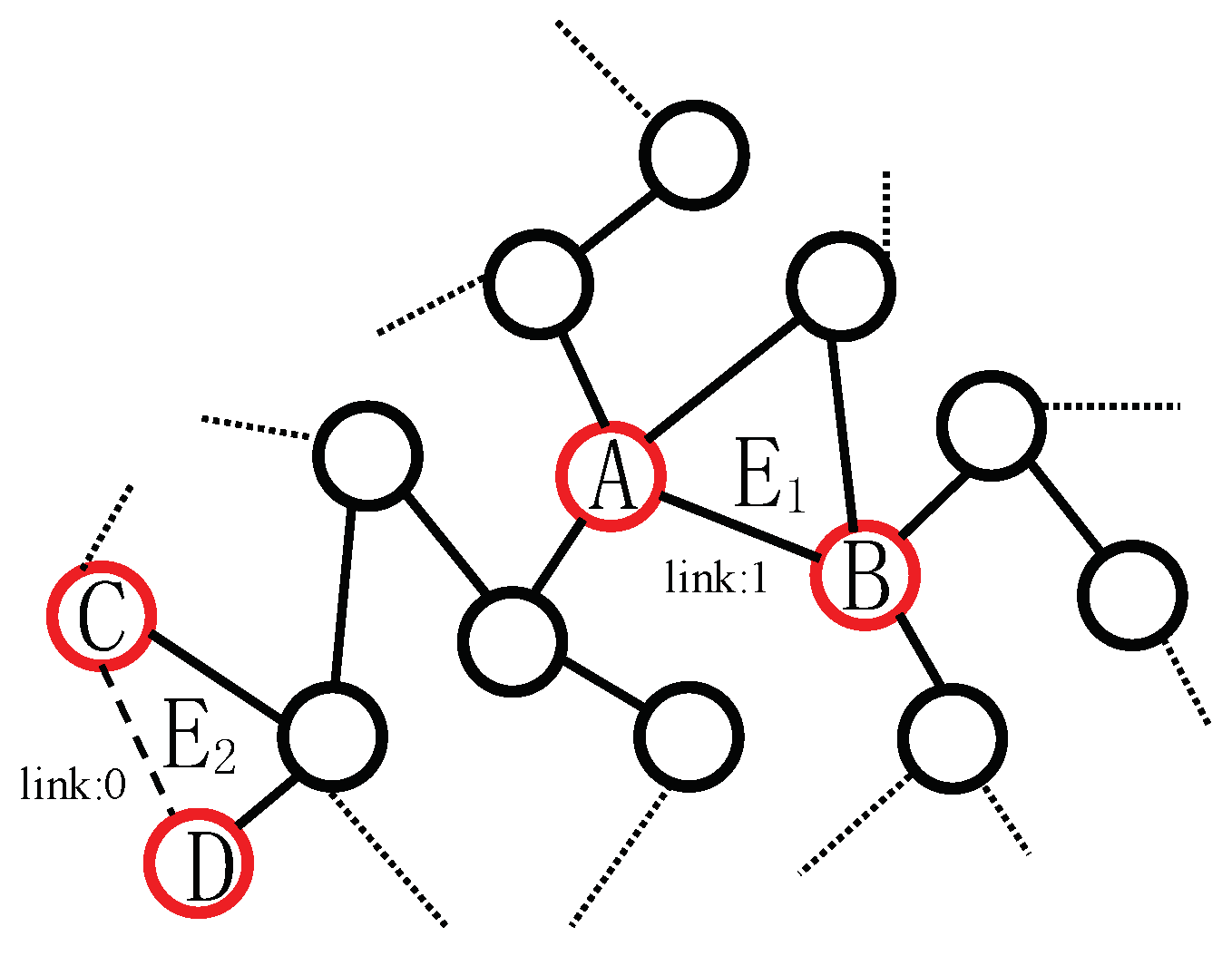
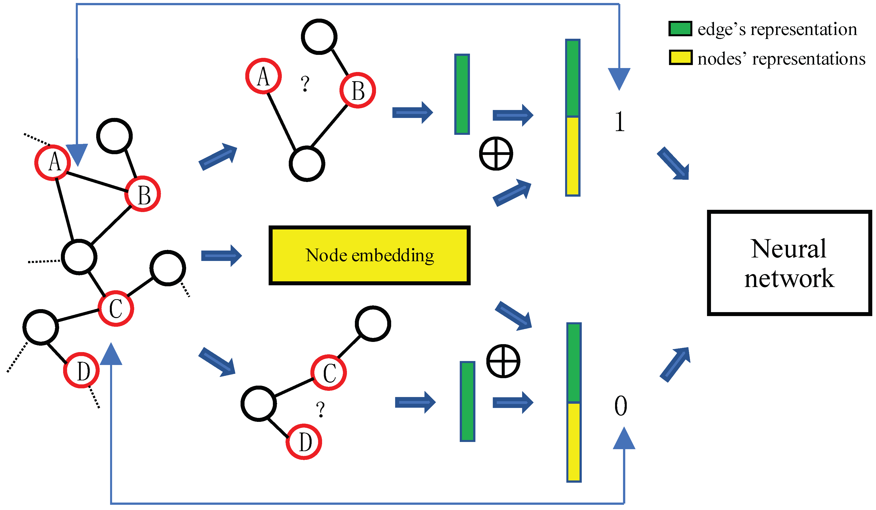
• We propose a new method to represent the link fully by combining the edge’s representation with the two nodes’ representations on the two sides of the edge, so that the neural network can learn abundant, meaningful patterns and link formation mechanism.

The rest of the paper is organized as follows. In Section 2, we discuss the related work, and in Section 3, we introduce our framework ENRNM in detail. The experiments and the results are presented in Section 4. Finally, we draw a conclusion and discuss the future work in Section 5.

2. Related Work

In the past few decades, link prediction has drawn lots of researchers’ attention. Many useful methods have been proposed for link prediction task, which can be divided into three categories: topological feature-based, latent feature-based and link embedding-based. The details are explained in the following.

Topological feature-based method extracts the features hidden inside the nodes and edges’ structures. A heuristic score is used to measure the similarity and connectivity between two nodes. Many heuristic methods perform very well on improving the accuracy of link prediction. Common neighbors (CN) [1] predicts link’s existence by the amounts of common neighbors of two nodes. Jaccard [21] considers that a link may exist when the common neighbors account for a high percentage of all neighbors of two nodes. Adamic-Adar (AA) [4] assumes that the common neighbors play an important role in a link’s formation if the neighbors’ number of these common neighbors is small. Besides, there are many other popular heuristic methods as shown in

Table 1. Popular heuristics for link prediction. $\mathsf{\Gamma }\left(x\right)$ is the neighbors set of node x. $l_{xy}^{+}$ is the $(x,y)$ entry of the pseudoinverse of the graph’s Laplacian matrix. ${\left[{\pi }_x\right]}_y$ is the stationary distribution probability of y under the random walk from x. $\beta$ is a damping factor whose value is less than 1. $walk{s}^l(x,y)$ denotes the number of l-length paths from x to y.

Method	Formula
common neighbors	$\left|\mathsf{\Gamma }\right(x)\cap \mathsf{\Gamma }(y\left)\right|$
Jaccard	${\displaystyle \frac{\left|\mathsf{\Gamma }\right(x)\cap \mathsf{\Gamma }(y\left)\right|}{\left|\mathsf{\Gamma }\right(x)\cup \mathsf{\Gamma }(y\left)\right|}}$
preferential attachment	$\left|\mathsf{\Gamma }\right(x\left)\right|\ast \left|\mathsf{\Gamma }\right(y\left)\right|$
Adamic-Adar	${\sum }_{z\in \mathsf{\Gamma }\left(x\right)\cap \mathsf{\Gamma }\left(y\right)}{\displaystyle \frac{1}{log\left(\mathsf{\Gamma }\right(z\left)\right)}}$
resource allocation	${\sum }_{z\in \mathsf{\Gamma }\left(x\right)\cap \mathsf{\Gamma }\left(y\right)}{\displaystyle \frac{1}{\left|\mathsf{\Gamma }\right(z\left)\right|}}$
resistance distance	${\displaystyle \frac{1}{l_{xx}^{+}+l_{yy}^{+}-2l_{xy}^{+}}}$
PageRank	${\left[{\pi }_x\right]}_y+{\left[{\pi }_y\right]}_x$
Katz	${\sum }_{l=1}^{\infty }{\beta }^l\left|walk{s}^l(x,y)\right|$

, empirical comparisons of these heuristics on different networks can be found in [22].

Latent feature-based method tends to get the representations and properties of nodes, which are often obtained in the way of factorizing a matrix [23] such as the adjacency matrix or the Laplacian matrix. Through factorizing a matrix, we can get the representation of each node in the form of a low-dimension vector. Then we can conduct the link prediction task by combining two nodes’ low-dimension vectors as link’s representation for each link. Latent feature-based methods focus on the individual nodes and miss the structural similarities between nodes, high-dimension vectors are needed if we want to utilize the heuristic information.

Link embedding-based method is an emerging approach, it learns a link’s formation mechanism from the network by itself other than assuming a particular mechanism (such as common neighbors). A typical method is WLNM [16] which extracts an enclosing subgraph for each link and encodes the subgraph to an adjacency matrix as link’s surrounding environment, namely the link’s representation. A neural network is trained to predict the link’s existence. The method is universal for the reason that it works well on almost all kinds of networks, and it outperforms many other methods. Another method SEAL [24] also performs pretty well on all kinds of networks. SEAL learns link’s formation mechanism from subgraph, node embedding, attributes and trains a graph neural network(GNN) for link prediction.

Another link embedding-based method does not acquire link embedding directly but represents the link by combining the two nodes’ representations on the two sides of the edge in different manners. Network embedding has been a hot topic recently because of the pioneering work DeepWalk [17]. DeepWalk uses random walks beginning from a node as a node sentence which is similar to a word sentence, then it trains a skip-gram model [25] to learn the node embedding of a specific network. Different from word embedding whose input is a significant corpus and output is almost all the words’ embeddings, network embedding method needs to learn node’s embedding for each network since these networks are isolated from each other. On the basis of the DeepWalk, Node2vec [18] and LINE [19] are developed to improve the performance of network embedding. And the low-dimension node embedding is useful in the tasks of visualization, network classification, community detection and link prediction.

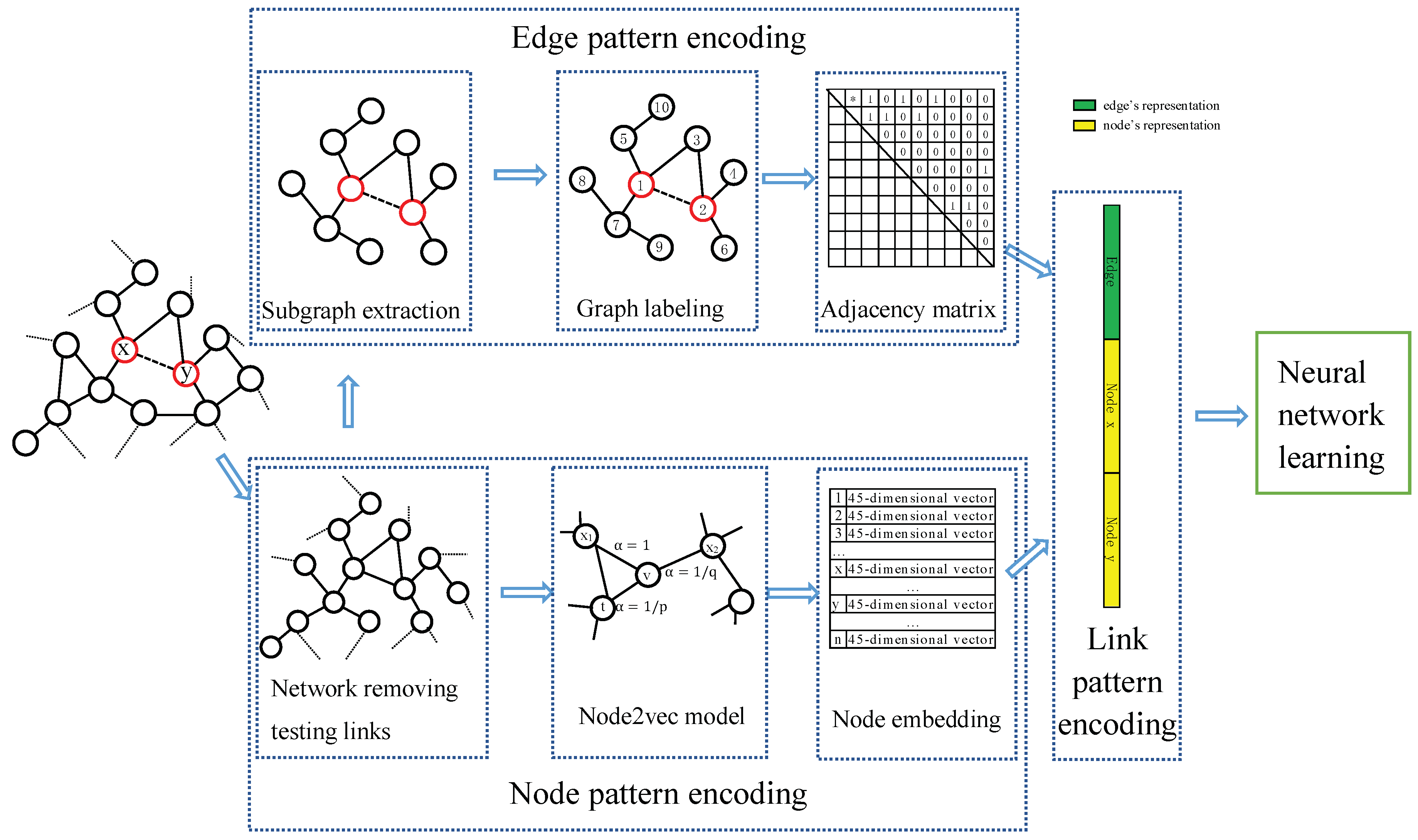
3. Edge-Nodes Representation Neural Machine (ENRNM)

In this section, we introduce the ENRNM in detail as shown in Figure 3. It includes four stages: edge pattern encoding, node pattern encoding, link pattern encoding and neural network learning.

ENRNM includes the following four main steps:

• Edge pattern encoding, which learns edge’s representation by WLNM.
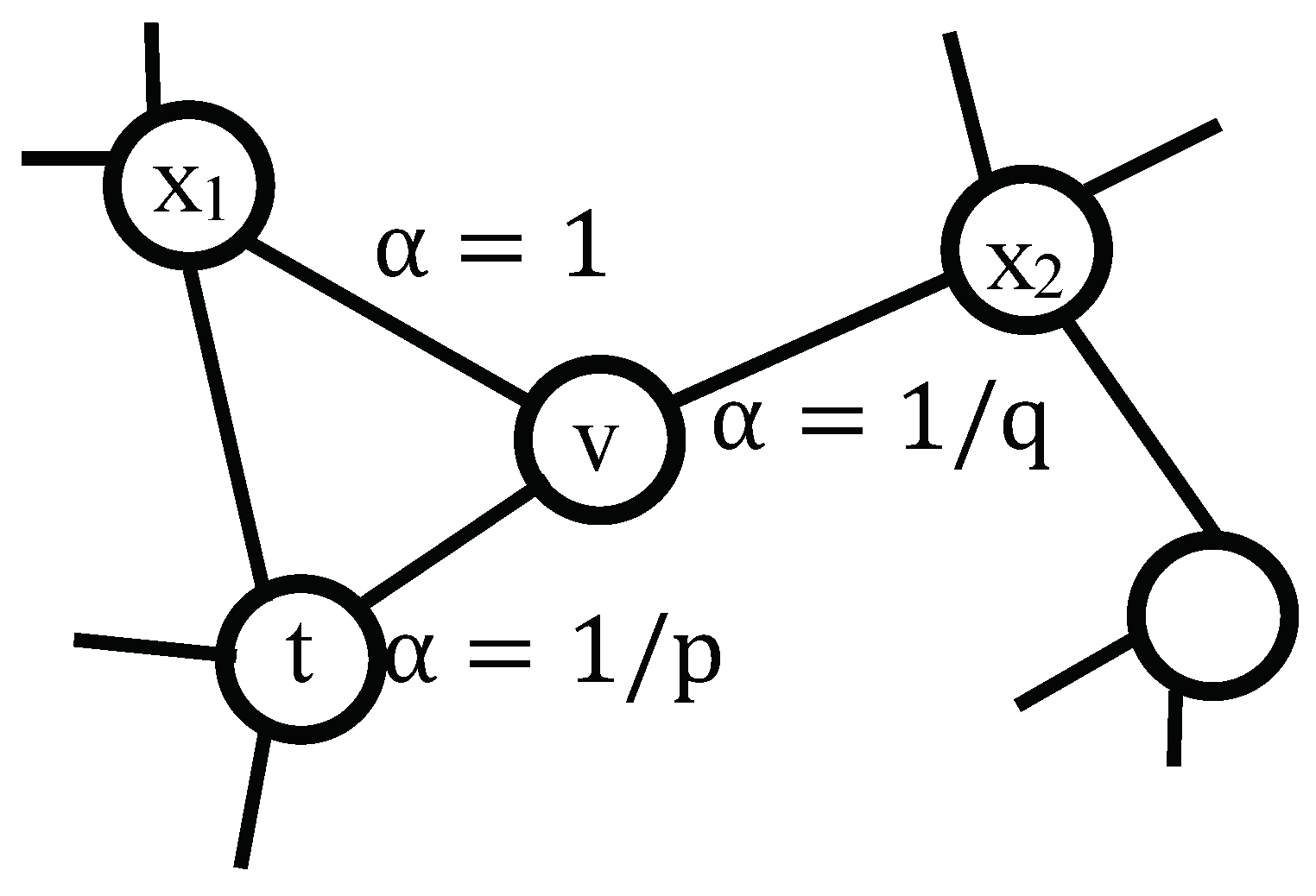
• Node pattern encoding, which learns node’s representation by network embedding model.
• Link pattern encoding, which joints the edge’s representation and two nodes’ on the two sides of the edge as link’s representation for each link.
• Train a fully connected neural network, which learns nonlinear graph topological structures and link’s formation mechanism for link prediction.

Our proposed method ENRNM is explained in the Algorithm 1.

The paper mainly focuses on the undirected and unweighted network. A network can be represented as an undirected and unweighted graph $G(V,E)$ where $V=\left\{v_1,v_2,v_3\dots v_n\right\}$ indicates the set of nodes and $E\subseteq V\times V$ indicates the set of edges observed. Nodes $v_1,v_2,v_3\dots v_n$ are integer numbers set manually and edges are presented in the form of $(v_i,v_j)$. In the graph, there is no self-loop and there is at most an edge between two nodes. A graph can be represented as an adjacency matrix A, $A_{ij}=1$ if there is a link between node $v_i$ and node $v_j$ and $A_{ij}=0$ otherwise. Adjacency matrix A is symmetric since the graph is undirected. We use $\mathsf{\Gamma }\left(x\right)$ or ${\mathsf{\Gamma }}^1\left(x\right)$ to indicate the set of all the neighbors of node x, in other words, ${\mathsf{\Gamma }}^1\left(x\right)$ is the set of the nodes whose distances to node x are equal to 1. We use ${\mathsf{\Gamma }}^n\left(x\right)$ to indicate the set of the nodes whose distances to node x are less than or equal to n.

Algorithm 1 ENRNM

Input: network G Output: AUC 1: devide the observed and unobserved links of network G into two parts: training and testing links 2: for each link $(x,y)$ do 3:     learn the edge’s representation $edgevec(x,y)$ 4:     learn the nodes’ representations $nodevec\left(x\right)$ and $nodevec\left(y\right)$ 5:     $linkvec(x,y)=joint\left(edgevec\right(x,y),nodevec(x),nodevec(y\left)\right)$ 6: end for 7: feed $linkvec(x,y)$ and label $(1:(x,y)\in E,0:(x,y)\notin E)$ to neural network for the training data 8: feed $linkvec(x,y)$ of the testing data to the pre-trained neural network 9: compare the predicted labels with real labels 10: return AUC value

3.1. Edge Pattern Encoding

To acquire the full representation for each link, we need to represent edges and nodes firstly. Traditional edge embedding methods tend to combine the representations of nodes on the two sides of the edge in different manners as link’s representation. But recently there are many new methods such as WLNM, it pays attention to get the surrounding environments of the edge. WLNM extracts a subgraph for each edge firstly then transforms the unordered subgraph to an ordered subgraph which can be represented as an adjacency matrix. The edge pattern encoding method is explained in the Algorithm 2, and the detail is elaborated in the following.

Algorithm 2 Edge pattern encoding

Input: network G, edge $(x,y)$, integer K Output: edge’s representation $edgevec(x,y)$ 1: $V_K=\left\{x,y\right\}$ 2: $temp$= $\left\{x,y\right\}$ 3: while$|V_K|<K$ and $\left|temp\right|>$0 do 4:     $temp=\left({\cup }_{v\in temp}\mathsf{\Gamma }\left(v\right)\right)\setminus V_K$ 5:     $V_K=V_K\cup temp$ 6: end while 7: calculate $d\left(v\right):=\sqrt{\left(d\right(v,x\left)d\right(v,y\left)\right)}$ for all $v\in V_K$ 8: get initial symbols $c\left(v\right)=f\left(d\right(v\left)\right)$ for all $v\in V_K$ 9: while$c\left(v\right)$ not converge do 10:     calculate hashing values $h\left(v\right)$ for all $v\in V_K$ 11:     update symbols $c\left(v\right)=f\left(d\right(v\left)\right)$ 12: end while 13: convert the labeled subgraph to an adjacency matrix 14: joint all the columns of upper triangle of adjacency matrix vertically and record as $edgevec(x,y)$ 15: return$edgevec(x,y)$

For each target edge between node x and node y, we extract a subgraph which can be considered as the edge’s surrounding environment and the nodes’ amount of the subgraph is K, a number set manually. Then we add node x, node y, $\mathsf{\Gamma }\left(x\right)$, $\mathsf{\Gamma }\left(y\right)$, ${\mathsf{\Gamma }}^1\left(x\right)$, ${\mathsf{\Gamma }}^1\left(y\right)$, ${\mathsf{\Gamma }}^2\left(x\right)$, ${\mathsf{\Gamma }}^2\left(y\right)$… into the subgraph until the nodes’ number of the subgraph is more than K or there are no more nodes to add.

After the subgraph extraction, we need to transform the unordered subgraph to an ordered subgraph by a graph labeling algorithm, then we can represent the subgraph as an adjacency matrix. Each node of the subgraph is given an initial symbol according to the distances to node x and node y, then we update the symbol iteratively determined by the hash function h and the mapping function f which can map a hash value to an integer.

The hash function is shown as Equation (1) [16]:

$$h\left(x\right)=c\left(x\right)+\frac{{\sum }_{z\subseteq \mathsf{\Gamma }\left(x\right)}log\left(p\left(c\left(z\right)\right)\right)}{{\sum }_{z^{{}^{\prime }}\subseteq V_K}log\left(p\left(c\left(z{}^{\prime }\right)\right)\right)}.$$

(1)

The hashing function is based on the Weisfeiler–Lehman algorithm [26], a color refinement algorithm which transforms an unordered graph to an ordered graph. In the Equation (1), c(x) is the current symbol of node x, $p\left(n\right)$ indicats the nth prime number, $p\left(1\right)=2$, $p\left(2\right)=3$, $p\left(3\right)=5$, $p\left(4\right)=7$… After getting an ordered subgraph, we can represent the subgraph as an adjacency matrix whose order is decided by the integer symbols. Generally, we often set $A_{ij}=1/0$ to indicate that there is a link between the corresponding two nodes i and j or not. To learn more meaningful patterns, we set $A_{ij}=function\left(d((i,j),(x,y))\right)$, where $d\left(\right(i,j),(x,y\left)\right)$ is the shortest distance between edge $(i,j)$ and edge $(x,y)$. In the end, we splice the upper triangle of the adjacency matrix vertically to a vector as the edge’s representation.

3.2. Node Pattern Encoding

In this section, we introduce the method of generating node’s representation. Node2vec works well in link prediction, therefore, we use Node2vec to generate node embedding in the node pattern encoding part of our method. Indeed, other network embedding methods are suitable too.

Node2vec changes the way of the random walk compared with DeepWalk. It uses two parameters, Return parameter p and In-out parameter q to control the next step of the walk, and the parameters settings can lead to different node sentences so the node embeddings. The parameter p controls the probability of visiting the previous node, and parameter q controls that the next step will visit a node which is close to the previous node or far away to it. As shown in Figure 4, the current node is node v, the previous node is node t, now we need to determine the next walk to which node selected from node t, node $x_1$ and node $x_2$. We choose the next node according to the distance between the node x and the previous node t. The transition probability is shown in Equation (2) [18].

The transition probability ${\alpha }_{pq}(t,x)$ is as following Equation (2).

$${\alpha }_{pq}(t,x)=\left\{\begin{array}{cc}1/p,\hfill & \mathrm{if} d_{tx}=0\hfill \\ 1,\hfill & \mathrm{if} d_{tx}=1\hfill \\ 1/q,\hfill & \mathrm{if} d_{tx}=2.\hfill \end{array}\right.$$

(2)

After random walk getting a node sentence for each node, we feed these node sentences to the skip-gram model to learn the node embedding. We illustrate the node pattern encoding algorithm in Algorithm 3. In the end, we get the embedding of each node in the form of vector.

Algorithm 3 Node pattern encoding

Input: network G, dimension d, walks per node r, walk length l, context size k, return p, in-out q Output: every node’s representation $nodevec$ 1: calculate transition probability ${\alpha }_{pq}(t,x)$ according to p, q and $d_{tx}$ 2: $\pi =PreprocessModifiedWeights(G,\alpha )$ 3: $G^{{}^{\prime }}=(V,E,\pi )$ 4: initialize walks to empty 5: for$i=1$ to r do 6:     for all nodes $u\in V$ do 7:         $walk=node2vecWalk(G^{{}^{\prime }},u,l)$ 8:         append walk to walks 9:     end for 10: end for 11: $nodevec=SGD(k,d,walks)$ 12: return$nodevec$

3.3. Link Pattern Encoding

After we get the edge’s representation $edgevec(x,y)$ and nodes’ representations $nodevec(x$), $nodevec\left(y\right)$ for target link $(x,y)$, then we can acquire the link’s representation by combining the edge and nodes’ representations. In our experiment, we convert $edgevec(x,y)$, $nodevec\left(x\right)$, $nodevec\left(y\right)$ to column vectors respectively and splice the three column vectors vertically to a long column vector as link’s full representation. The order of the three column vectors is $edgevec(x,y)$, $nodevec\left(x\right)$, $nodevec\left(y\right)$ and the integer value of x is small than that of y.

3.4. Neural Network Learning

3.4.1. Training

After getting the link’s representation, the last step is training a classifier which can predict the existence of the link. We choose a fully connected neural network to learn complicated nonlinear patterns for the reason that the neural network has powerful learning ability to fit our training data.

For the given network $G=(V,E)$, the training dataset includes positive samples which are randomly selected from the observed links and negative samples which are randomly chosen from the unobserved links, as same as the testing dataset. And the number of negative samples is twice of the number of positive samples. For a given training link $(x,y)$, regardless of positive or negative, ENRNM firstly learns the edge $(x,y)$, node x and node y’ representations respectively by the corresponding methods, then combines them vertically as link’s representation. In the end, the training links’ vector representations are fed into neural network together with their labels $(1:(x,y)\in E,0:(x,y)\notin E)$ to train the model.

3.4.2. Testing (Link Prediction)

After training the neural network and getting a nonlinear classifier, we can use the classifier to predict the existence of a testing link by representing its corresponding edge and nodes, combining the three representations vertically and feeding it into the pre-trained neural network. Then the classifier outputs two scores whose values are between 0 and 1, and the sum of them is 1. The two scores indicate the probability of link’s existence or not. In the end, we compare the predicted labels with the actual labels of the testing samples and use the area under the ROC curve (AUC) to evaluate the link prediction’s effect.

4. Experiments and Results

In this section, we conduct comprehensive experiments to evaluate the performance of ENRNM, we compare it with 14 baselines on eight real-world networks. The result indicates that ENRNM combining edge and two nodes’ representations as link’s representation outperforms many other methods.

4.1. Datasets

In our experiments, there are eight datasets with different structures and characteristics including C.ele [2], USAir [27], PB [28], NS [29], E.coli [30], Yeast [3], Power [2] and Router [31]. The numbers of edges and nodes of each dataset are shown in

Table 2. The nodes and edges’ numbers of all the datasets.

Datasets	|V|	|E|
C.ele	297	2148
USAir	332	2126
PB	1222	16,714
NS	1589	2742
E.coli	1805	14,660
Yeast	2375	11,693
Power	4941	6594
Router	5022	6258

. C.ele is a neural network of C. elegans, whose nodes indicate neurons, synapses and edges indicate that there are excitement signals between neurons and synapses. USAir is a network of United States Airlines, whose nodes indicate different cities and edges indicate the airlines between these cities. PB is a network of America political blogs, whose nodes indicate political blogs and edges are automatically extracted from a crawl of the front page of the blog. NS is a collaboration network of researchers in network science, whose nodes indicate different researchers and edges indicate that two researchers have published papers cooperatively. E.coli is a pairwise reaction network of metabolites in E.coli, whose nodes indicate metabolites of E.coli and edges indicate reaction among metabolites. Yeast is a protein-protein interaction network in yeast, whose nodes indicate proteins of yeast and edges indicate that there are interactions between proteins. Power is an electrical network of western US, whose nodes indicate transformers, substations, generators and edges indicate high-voltage transmission lines. Router is a router–Level internet, whose nodes indicate various routing devices and edges indicate that there are data transmissions between these routing devices.

4.2. Baselines and Experimental Setting

Supposing that the numbers of nodes and edges of a network are n and m respectively, there are at most $n\ast (n-1)/2$ links in the network, and m links of them are observed and $n\ast (n-1)/2-m$ links are unobserved. For each dataset, we divide the observed links called positive samples into two parts. Training set accounts for ninety percent and testing set accounts for ten percent. For the training set, we sample negative training samples from the unobserved links and set its number to be twice of the number of positive training samples, as same as the testing set. We remove these testing links from the network, and we try to find out these missing links especially these positive testing links.

We adopt AUC (area under the ROC curve) to evaluate the performance of link prediction, which is used frequently to evaluate the effect of binary classifier. AUC is equivalent to the probability that a randomly chosen positive example is ranked higher than a randomly selected negative example. AUC considers the ability of classifying positive and negative samples simultaneously, each sample is classified correctly if AUC is 1. To speak more intuitively, when we get a higher AUC value, indicating that the classifier can classify both positive sample and negative sample more accurately. AUC is not sensitive to whether it is unbalanced between the amounts of positive and negative samples.

For the proposed method ENRNM, we set the nodes’ amount of the subgraph as 10, which performs better than other integer settings when generating the representation of the edge. So the dimension of the edge’s vector is $10\times (10-1)/2=45$. And when generating the node’s representation, the dimension of the node’s vector is 45 too. The reason why we make these settings is that we want to express the idea that edge and nodes on the two sides of the edge have the same importance in representing a link. Besides, the Return parameter p and the In-out parameter q both is equal to 1. In the setting, node2vec randomly walks in the graph and gives the same chance to the nodes which are near to the current node to be added into the node sentence.

For the same training data, classifiers trained by various models are different. Before we determine using the neural network to learn link’s formation mechanism, we conduct a series of experiments to find the most suitable classifier. The classifiers we use include logistic regression [32], decision tree [33], random forest [34], adaboost [35] and neural network. For random forest classifier, there are 100 trees in the forest. For the neural network, we use the structure of three fully connected layers with 32, 32, 16 hidden units, respectively. And in the end, we use SoftMax layer to output two probability values indicating whether there is a link or not. The activation function in the neural network we use is Rectified Linear Unit (ReLU). And we adopt the Adam update rule [36] for optimization with a learning rate of 0.001 at the beginning whose drop ratio is 0.9, a mini-batch size of 128, the training epochs of 200. To avoid overfitting, we use Dropout [37] and Early-stopping to learn more useful patterns. All the above are implemented by the neural network tool of MATLAB. The AUC results of different classifiers are shown in

Table 3. AUC results of different classifiers for ENRNM.

Datasets	Logistic Regression	Decision Tree	Random Forest	Adaboost	Neural Network
C.ele	0.8429	0.7186	0.757	0.7581	0.870
USAir	0.958	0.8697	0.8803	0.8756	0.968
PB	0.937	0.7992	0.8663	0.8488	0.9453
NS	0.937	0.9273	0.9345	0.9218	0.9832
E.coli	0.9563	0.8762	0.9212	0.889	0.9787
Yeast	0.9378	0.8861	0.9066	0.8878	0.9618
Power	0.7968	0.6534	0.6924	0.6693	0.866
Router	0.9134	0.6158	0.623	0.7768	0.921

, we can see that the neural network is the most suitable classifier. Therefore, in the next experiments, we use the neural network as our classifier to learn meaningful and abundant patterns.

In our experiments, we compare our method ENRNM with twelve heuristics including common neighbors (CN) [1], Jaccard (Jac.) [21], Adamic-Adar (AA) [4], resource allocation (RA) [11], preferential attachment (PA) [10], Katz [12], resistance distance (RD) [14], PageRank (PR) [1], SimRank (SR) [13], Stochastic block model (SBM) [9], matrix factorization using a classification loss function (MF-c) [23], matrix factorization using a regression loss function (MF-r) [23], and two popular methods including WLNM [16] which employs edge’ representation as link’s formation mechanism and Node2vec [18] which combines two nodes’ embeddings on the two sides of the edge as link’s formation mechanism. For some methods, different parameter settings lead to unequal results and we often use the best results. For Katz, we set the damping factor $\beta$ to 0.001 and for PageRank, we set the damping factor to 0.85, which is suggested in the [16]. For SBM, we adopt the implementation straightly in [38], where the number of latent groups is chosen in $\left\{4,6,8,10,12\right\}$. For MF, we utilize the libFM [39] software, where the number of latent factors of MF is searched in $\left\{5,10,15,20,50\right\}$. For WLNM, we set the nodes’ number K of subgraph to 10, which is presented to have good performance on different networks. For Node2vec, we generate 45-dimension vector as node embedding.

To show our results more intuitively, we draw a line chart according to the corresponding result table. We conduct two groups experiments. The first group experiments compare the heuristic methods with the proposed method ENRNM as shown in Table 6 and Figure 8, the second group experiments compare the Node2vec, WLNM and ENRNM as shown in Table 7 and Figure 9. Moreover, we analyze the characteristics of heuristics, Node2vec, WLNM and ENRNM in

Table 4. Characteristics comparison of differnent link prediction methods.

Features	Heuristics	Node2vec	WLNM	ENRNM
Graph structure feature	Yes	Yes	Yes	Yes
Node’s information	No	Yes	No	Yes
Edge’s information	No	No	Yes	Yes
Model	/	NN	NN	NN

. In Figure 5, we compare the link’s representation of Node2vec, WLNM and ENRNM.

We draw a weight graph for the dataset USAir to prove that the edge and two nodes have the same importance in the formation of the link. The dimension of edge and two nodes’ vector representations is 45, and there are 32 units in the first hidden layer, so the size of weight matrix from the input layer to the first hidden layer is $135\times 32$. As shown in Figure 6, the horizontal axis denotes the first hidden layer with 32 units, the vertical axis denotes the sum of absolute values of 45 weights of each feature to the corresponding hidden unit. We can observe that almost all the weights are more than 2, and the tendencies of the three lines are similar. Moreover, the weights of the three features are similar indicating that the three feature representations play the same important role in link’s formation. So combining the edge and two nodes’ representations as link’s formation is useful to improve the link prediction performance.

4.3. Time and Computational Complexity

We compare the computational complexity and time needed in the process of link representation of the methods WLNM, Node2vec and ENRNM in

Table 5. The processes and computational complexity per sample. And we calculate the time needed in the process of link representaion for dataset USAir. K indicates the nodes’ amount of subgraph. l denotes the walk length, k indicates the context size. n denotes the amount of nodes of the network.

Methods	Process	Computational Complexity/Sample	Time Needed (s)
WLNM	edge (link) pattern encoding	$O\left(K^3\right)$	44.912
Node2vec	node pattern encoding link pattren encoding	$O\left(l/k\left(l-k\right)\right)$ $O\left(n\right)$	10.326 0.500
ENRNM	node pattern encoding edge pattern encoding link pattren encoding	$O\left(l/k\left(l-k\right)\right)$ $O\left(K^3\right)$ $O\left(n\right)$	10.628 46.646 1.000

. Since our method combines the edge and nodes’ representations so we need to spend a little more time to build link’s representation, and our method is a bit more complex than WLNM and Node2vec. Actually, the time needed of ENRNM to encode link pattern is less than 1 min. Fortunately, our method achieves the best batch accuracy and the smallest batch loss quicker (shown in Figure 7) in the process of training due to the full representation of link. Therefore we always set max epoch as 100 or 150 which is enough to learn a useful model, shortening the time of training largely for ENRNM.

4.4. Results

From the

Table 6. AUC results of 12 baselines and ENRNM.

Datesets	CN	Jac	AA	RA	PA	Katz	RD	PR	SR	SBM	MF-c	MF-r	ENRNM
C.ele	0.849	0.793	0.863	0.867	0.756	0.865	0.741	0.902	0.761	0.866	0.838	0.843	0.870
USAir	0.941	0.904	0.949	0.957	0.893	0.930	0.897	0.943	0.783	0.945	0.919	0.845	0.968
PB	0.92	0.874	0.923	0.922	0.9012	0.927	0.882	0.934	0.772	0.937	0.933	0.942	0.9453
NS	0.939	0.939	0.939	0.937	0.6823	0.941	0.583	0.941	0.941	0.921	0.638	0.721	0.9832
E.coli	0.933	0.807	0.953	0.959	0.913	0.928	0.887	0.952	0.638	0.938	0.906	0.918	0.9787
Yeast	0.892	0.891	0.892	0.893	0.825	0.922	0.881	0.926	0.915	0.915	0.839	0.883	0.9618
Power	0.592	0.591	0.592	0.591	0.442	0.656	0.844	0.665	0.762	0.664	0.522	0.515	0.866
Router	0.561	0.562	0.561	0.562	0.472	0.379	0.925	0.381	0.368	0.852	0.775	0.782	0.921

and Figure 8, we can get the conclusion as follows. Compared with other 12 heuristic methods, our proposed method ENRNM achieves unparalleled performance across eight networks with different structures and characteristics in terms of AUC. Our method performs well on almost all the datasets indicating that the method is universal and suitable for almost all kind of networks. Most remarkably, ENRNM performs extremely well on the datasets Power and Router, on which many other heuristic methods’ performances are just better than random guessing. For the datasets C.ele and Router, the method PR and RD achieve a bit better performance than our method. However as noticed in Table 6, the methods RD and PR perform poorly on several datasets, they are not universal methods. The method we propose is suitable for almost all the datasets since we gain good effect on all the datasets, although we cannot achieve the best performance on two datasets. In terms of these eight different kinds of datasets, we believe that our method ENRNM is suitable for all kinds of networks and it can achieve enough good performance though may not be the best for some datasets. The red line in Figure 8 indicates the result of our method ENRNM, and we can observe that the red line is the top of almost all the lines.

Observing the

Table 7. AUC results of Node2vec, WLNM and ENRNM.

Datasets	Node2vec	WLNM	ENRNM
C.ele	0.6604	0.859	0.870
USAir	0.8477	0.958	0.968
PB	0.9168	0.933	0.9453
NS	0.9657	0.984	0.9832
E.coli	0.9691	0.971	0.9787
Yeast	0.9524	0.956	0.9618
Power	0.8567	0.848	0.866
Router	0.640	0.944	0.921

and Figure 9, we can conclude that the method Node2vec performs well on several datasets, and WLNM achieves the best performance on the datasets NS and Router. For the datasets NS and E.coli, the three methods including Node2vec, WLNM and ENRNM achieve good effects. For six datasets, the method ENRNM has the best performance indicating that we represent the link fully and the neural network learns the most important and meaningful patterns. For dataset Router, the performance of method WLNM is a little better than ours, but the effect of Node2vec is unsatisfactory, we consider that the node pattern encoding generated by Node2vec method may be not suitable for Router. All in all, our method achieves quite good performance on diverse networks with different structures and characteristics. The red line in Figure 9 indicates the result of ENRNM, and we can see that the red line is the top of almost all the lines.

5. Conclusions and Future Work

5.1. Conclusions

In this paper, we propose a novel and universal link prediction method Edge-Nodes Representation Neural Machine (ENRNM), which learns topological features fully from networks by combining the representations of edge and nodes on the two sides of the edge as link’s representation, namely formation mechanism. We represent the link fully so that the neural network can learn abundant and meaningful patterns. Experiment results show that ENRNM has superb performance when comparing with fourteen state-of-the-art methods across diverse networks with different structures and characteristics, especially the WLNM method which just employs edge’s representation as link’s formation mechanism and the Node2vec method which only applies node’s representation as link’s formation mechanism.

5.2. Future Work

As shown in Table 7, we can see that the performance of Node2vec is not very perfect on some networks which may be caused by insufficient representation of node, leading to imperfect performance on ENRNM. Therefore in the future, we are committed to finding or creating more effective node pattern encoding method to improve our method ENRNM.

For the method ENRNM, we need to learn edge and two nodes’ representations respectively for each link, then combine them as link’s representation. In this way, the process of representing the link is sort of complicated. In the future, we will contribute to creating a new method to represent each link that includes edge and two nodes’ information to simplify the computing process. Besides, we will pay more attention to improve the link prediction performance of the datasets C.ele and Power on which the ENRNM and other state-of-the-art methods have poor performance.

References

1. Liben-Nowell, D.; Kleinberg, J. The link-prediction problem for social networks. J. Am. Soc. Inf. Sci. Technol. 2007, 58, 1019–1031. [Google Scholar] [CrossRef] [Green Version]
2. Kipf, T.N.; Welling, M. Semi-supervised classification with graph convolutional networks. arXiv, 2016; arXiv:1609.02907. [Google Scholar]
3. Von Mering, C.; Krause, R.; Snel, B.; Cornell, M.; Oliver, S.G.; Fields, S.; Bork, P. Comparative assessment of large-scale data sets of protein–protein interactions. Nature 2002, 417, 399. [Google Scholar] [CrossRef]
4. Adamic, L.A.; Adar, E. Friends and neighbors on the Web. Soc. Netw. 2003, 25, 211–230. [Google Scholar] [CrossRef] [Green Version]
5. Koren, Y.; Bell, R.; Volinsky, C. Matrix factorization techniques for recommender systems. Computer 2009, 42, 30–37. [Google Scholar] [CrossRef]
6. Nickel, M.; Murphy, K.; Tresp, V.; Gabrilovich, E. A review of relational machine learning for knowledge graphs. Proc. IEEE 2016, 104, 11–33. [Google Scholar] [CrossRef]
7. Oyetunde, T.; Zhang, M.; Chen, Y.; Tang, Y.; Lo, C. BoostGAPFILL: Improving the fidelity of metabolic network reconstructions through integrated constraint and pattern-based methods. Bioinformatics 2016, 33, 608–611. [Google Scholar] [CrossRef] [PubMed]
8. Salakhutdinov, R.; Mnih, A. Bayesian probabilistic matrix factorization using Markov chain Monte Carlo. In Proceedings of the 25th International Conference on Machine Learning, Helsinki, Finland, 5–9 July 2008; ACM: New York, NY, USA, 2008; pp. 880–887. [Google Scholar] [Green Version]
9. Airoldi, E.M.; Blei, D.M.; Fienberg, S.E.; Xing, E.P. Mixed membership stochastic blockmodels. J. Mach. Learn. Res. 2008, 9, 1981–2014. [Google Scholar] [PubMed]
10. Barabási, A.L.; Albert, R. Emergence of scaling in random networks. Science 1999, 286, 509–512. [Google Scholar]
11. Zhou, T.; Lü, L.; Zhang, Y.C. Predicting missing links via local information. Eur. Phys. J. B 2009, 71, 623–630. [Google Scholar] [CrossRef] [Green Version]
12. Katz, L. A new status index derived from sociometric analysis. Psychometrika 1953, 18, 39–43. [Google Scholar] [CrossRef]
13. Jeh, G.; Widom, J. SimRank: A measure of structural-context similarity. In Proceedings of the eighth ACM SIGKDD International Conference on Knowledge Discovery and Data Mining, Edmonton, AB, Canada, 23–26 July 2002; ACM: New York, NY, USA, 2002; pp. 538–543. [Google Scholar]
14. Klein, D.J.; Randić, M. Resistance distance. J. Math. Chem. 1993, 12, 81–95. [Google Scholar] [CrossRef]
15. Lü, L.; Zhou, T. Link prediction in complex networks: A survey. Phys. A Stat. Mech. Appl. 2011, 390, 1150–1170. [Google Scholar] [CrossRef] [Green Version]
16. Zhang, M.; Chen, Y. Weisfeiler–Lehman neural machine for link prediction. In Proceedings of the 23rd ACM SIGKDD International Conference on Knowledge Discovery and Data Mining, Halifax, NS, Canada, 13–17 August 2017; ACM: New York, NY, USA, 2017; pp. 575–583. [Google Scholar]
17. Perozzi, B.; Al-Rfou, R.; Skiena, S. DeepWalk: Online Learning of Social Representations. arXiv, 2014; arXiv:1403.6652. [Google Scholar]
18. Grover, A.; Leskovec, J. node2vec: Scalable feature learning for networks. In Proceedings of the 22nd ACM SIGKDD International Conference on Knowledge Discovery and Data Mining, San Francisco, CA, USA, 13–17 August 2016; ACM: New York, NY, USA, 2016; pp. 855–864. [Google Scholar]
19. Tang, J.; Qu, M.; Wang, M.; Zhang, M.; Yan, J.; Mei, Q. LINE: Large-scale Information Network Embedding. arXiv, 2015; arXiv:1503.03578. [Google Scholar]
20. Cai, H.; Zheng, V.W.; Chang, K.C. A Comprehensive Survey of Graph Embedding: Problems, Techniques and Applications. arXiv, 2017; arXiv:1709.07604. [Google Scholar]
21. Jaccard, P. Etude de la distribution florale dans une portion des Alpes et du Jura. Bulletin De La Societe Vaudoise Des Sciences Naturelles 1901, 37, 547–579. [Google Scholar]
22. Cukierski, W.; Hamner, B.; Yang, B. Graph-based features for supervised link prediction. In Proceedings of the 2011 IEEE International Joint Conference on Neural Networks (IJCNN), San Jose, CA, USA, 31 July–5 August 2011; pp. 1237–1244. [Google Scholar]
23. Miller, K.; Jordan, M.I.; Griffiths, T.L. Nonparametric latent feature models for link prediction. In Proceedings of the Advances in Neural Information Processing Systems, Vancouver, BC, Canada, 7–10 December 2009; pp. 1276–1284. [Google Scholar]
24. Zhang, M.; Chen, Y. Link Prediction Based on Graph Neural Networks. arXiv, 2018; arXiv:1802.09691. [Google Scholar]
25. Mikolov, T.; Sutskever, I.; Chen, K.; Corrado, G.; Dean, J. Distributed Representations of Words and Phrases and their Compositionality. arXiv, 2013; arXiv:1310.4546. [Google Scholar]
26. Weisfeiler, B.; Lehman, A. A reduction of a graph to a canonical form and an algebra arising during this reduction. Nauchno-Technicheskaya Informatsia 1968, 2, 12–16. [Google Scholar]
27. USAir Dataset. Available online: http://web.mit.edu/airlinedata/www/default.html (accessed on 2 January 2019).
28. Ackland, R. Mapping the Us Political Blogosphere: Are Conservative Bloggers More Prominent? BlogTalk Downunder 2005 Conference, Sydney. Available online: https://core.ac.uk/download/pdf/156616040.pdf (accessed on 2 January 2019).
29. Newman, M.E. Finding community structure in networks using the eigenvectors of matrices. Phys. Rev. E 2006, 74, 036104. [Google Scholar] [CrossRef] [PubMed] [Green Version]
30. Zhang, M.; Cui, Z.; Oyetunde, T.; Tang, Y.; Chen, Y. Recovering Metabolic Networks using A Novel Hyperlink Prediction Method. arXiv, 2016; arXiv:1610.06941. [Google Scholar]
31. Spring, N.; Mahajan, R.; Wetherall, D. Measuring ISP topologies with Rocketfuel. ACM SIGCOMM Comput. Commun. Rev. 2002, 32, 133–145. [Google Scholar] [CrossRef]
32. Peduzzi, P.; Concato, J.; Kemper, E.; Holford, T.R.; Feinstein, A.R. A simulation study of the number of events per variable in logistic regression analysis. J. Clin. Epidemiol. 1996, 49, 1373–1379. [Google Scholar] [CrossRef]
33. Safavian, S.R.; Landgrebe, D. A survey of decision tree classifier methodology. IEEE Trans. Syst. Man Cybern. 1991, 21, 660–674. [Google Scholar] [CrossRef] [Green Version]
34. Liaw, A.; Wiener, M. Classification and regression by randomForest. R News 2002, 2, 18–22. [Google Scholar]
35. Freund, Y.; Schapire, R. A short introduction to boosting. J. Jpn. Soc. Artif. Intell. 1999, 14, 1612. [Google Scholar]
36. Bengio, Y.; Louradour, J.; Collobert, R.; Weston, J. Curriculum learning. In Proceedings of the 26th Annual International Conference on Machine Learning, Montreal, QC, Canada, 14–18 June 2009; ACM: New York, NY, USA, 2009; pp. 41–48. [Google Scholar]
37. Srivastava, N.; Hinton, G.; Krizhevsky, A.; Sutskever, I.; Salakhutdinov, R. Dropout: A Simple Way to Prevent Neural Networks from Overfitting. J. Mach. Learn. Res. 2014, 15, 1929–1958. [Google Scholar]
38. Chen, Y.Y.; Gan, Q.; Suel, T. Local methods for estimating pagerank values. In Proceedings of the thirteenth ACM International Conference on Information and Knowledge Management, Washington, DC, USA, 8–13 November 2004; ACM: New York, NY, USA, 2004; pp. 381–389. [Google Scholar]
39. Rendle, S. Factorization machines with libfm. ACM Trans. Intell. Syst. Technol. (TIST) 2012, 3, 57. [Google Scholar] [CrossRef]
Figure 1. A link’s formation.
Algorithms 12 00012 g001
Figure 2. The ENRNM framework, the green strips indicate the edges’ representations generated from the subgraphs and the yellow strips indicate the nodes’ representations. For each target link, we combine the edge and two nodes’ representations as link’s representation namely formation mechanism. A neural network is used to predict whether the link exists.
Algorithms 12 00012 g002
Figure 3. Illustration of the method ENRNM including edge pattern encoding, node pattern encoding, link pattern encoding and neural network learning. Due to the space limitation of matrix in the figure, I expound the 45-dimensional vector here. For instance, the vector representation of the node 1 is 0.28701 , 0.1449 , 0.26971 0.61898 , 0.031769 , 041929 for dataset USAir.
Algorithms 12 00012 g003
Figure 4. Illustration of the random walk procedure in node2vec. The walk just transitioned from t to v and is now evaluating its next step out of node v. Edge labels indicate search biases α .
Algorithms 12 00012 g004
Figure 5. Link’s representation comparisons of WLNM, Node2vec and ENRNM.
Algorithms 12 00012 g005
Figure 6. Weight graph from the input layer to the first hidden layer.
Algorithms 12 00012 g006
Figure 7. Batch accuracy (a) and batch loss (b) varying along with the epoch of dataset USAir.
Algorithms 12 00012 g007
Figure 8. AUC results of 12 baselines and ENRNM.
Algorithms 12 00012 g008
Figure 9. AUC results of Node2vec, WLNM and ENRNM.
Algorithms 12 00012 g009