Performance Optimal PI controller Tuning Based on Integrating Plus Time Delay Models

Abstract

A method for tuning PI controller parameters, a prescribed maximum time delay error or a relative time delay error is presented. The method is based on integrator plus time delay models. The integral time constant is linear in the relative time delay error, and the proportional constant is seen inversely proportional to the relative time delay error. The keystone in the method is the method product parameter, i.e., the product of the PI controller proportional constant, the integral time constant, and the integrator plus time delay model, velocity gain. The method product parameter is found to be constant for various PI controller tuning methods. Optimal suggestions are given for choosing the method product parameter, i.e., optimal such that the integrated absolute error or, more interestingly, the Pareto performance objective (i.e., integrated absolute error for combined step changes in output and input disturbances) is minimised. Variants of the presented tuning method are demonstrated for tuning PI controllers for motivated (possible) higher order process model examples, i.e., the presented method is combined with the model reduction step (process–reaction curve) in Ziegler–Nichols.

1. Introduction

This paper concerns tuning of PI controllers based on Integrator Plus Time Delay (IPTD) models/systems. Further details and developments regarding the $\delta$-tuning algorithm are presented in the work [1,2]. IPTD processes and close-to IPTD systems are important/typical processes/systems found in the industry. Instances of IPTD processes are pulp and paper mills, oil water gas separators, communication networks, level systems and all lag-dominant processes, which may be approximated by IPTD models (see, e.g., [3,4,5]). Reported instances are high-purity distillation columns where there are relatively large time constants for minor differences in the reference, and where the time delay comes from an analyser (see, e.g., [6,7]). In Section 6.4 in [8], an example of reboiler control in connection with a distillation column was presented.

The majority of existing PI controller tuning rules for IPTD processes,

$$\begin{array}{c}\hfill H_p\left(s\right)=\frac{k}{s}{e}^{-\tau s},\end{array}$$

(1)

may be written as the following setting

$$\begin{array}{c}\hfill K_p=\frac{\alpha }{k\tau },T_i=\beta \tau ,\end{array}$$

(2)

where $K_p$ is the PI controller proportional gain, $T_i$ is the integral time constant, k is the gain velocity (slope) and $\tau \ge 0$ is the time delay. $\alpha$ and $\beta$ in Equation (2) are dimensionless parameters. For instance, using the classical Ziegler–Nichols (ZN) PI controller tuning rules, proposed in the works [9,10,11], gives $\alpha =\frac{\pi }{4.4}$, $\beta =\frac{4}{1.2}$ (i.e., the ZN closed loop method). Using the Internal Model Control (IMC) PI controller tuning rules in Table 1 of [7] with closed loop time constant $T_c=\sqrt{10}\tau$, as proposed in [6], gives parameters $\alpha =0.42$ and $\beta =7.32$. Using the Simple/Skogestad IMC (SIMC) PI controller tuning rules, presented in the works of [8,12,13], with closed loop time constant $T_c=\tau$ (i.e., is the only tuning parameter in SIMC) gives $\alpha =0.5$ and $\beta =8$.

Table 1. The table shows the recommended MP parameters $\overline{c}$ if one wants to minimise the main performance objective $V_M$ (Equation (42)) for different servo-regulator parameters $s_r$ in Equation (41). The optimal $\overline{c}$ values as indicated are almost constant in the interval $\delta \in [1.1,3.4]$ ([2]).

${\mathit{s}}_{\mathit{r}}$	0	0.1	0.25	0.5	0.75	1
$\overline{c}$	2.4	2.5	2.6	2.7	3.7	∞

To find PI controller settings with good robustness properties (i.e., one could have uncertainties in the gain velocity and time delay) and simultaneously obtain reasonable fast reference and disturbance properties, for IPTD processes, the size and balanced relation between the parameters $\alpha$ and $\beta$ are of importance.

Using the PI controller setting in Equation (2), we may define a Method Product (MP) parameter $\overline{c}$ as,

$$\begin{array}{c}\hfill \overline{c}=\alpha \beta =K_p{T}_{i}k.\end{array}$$

(3)

The defined MP parameter $\overline{c}$ in Equation (3) is constant for numerous PI controller tuning methods. The SIMC PI controller settings yield an MP parameter $\overline{c}=4$. The original ZN method gives an MP parameter $\overline{c}=2.38$ (i.e., the ZN closed loop method).

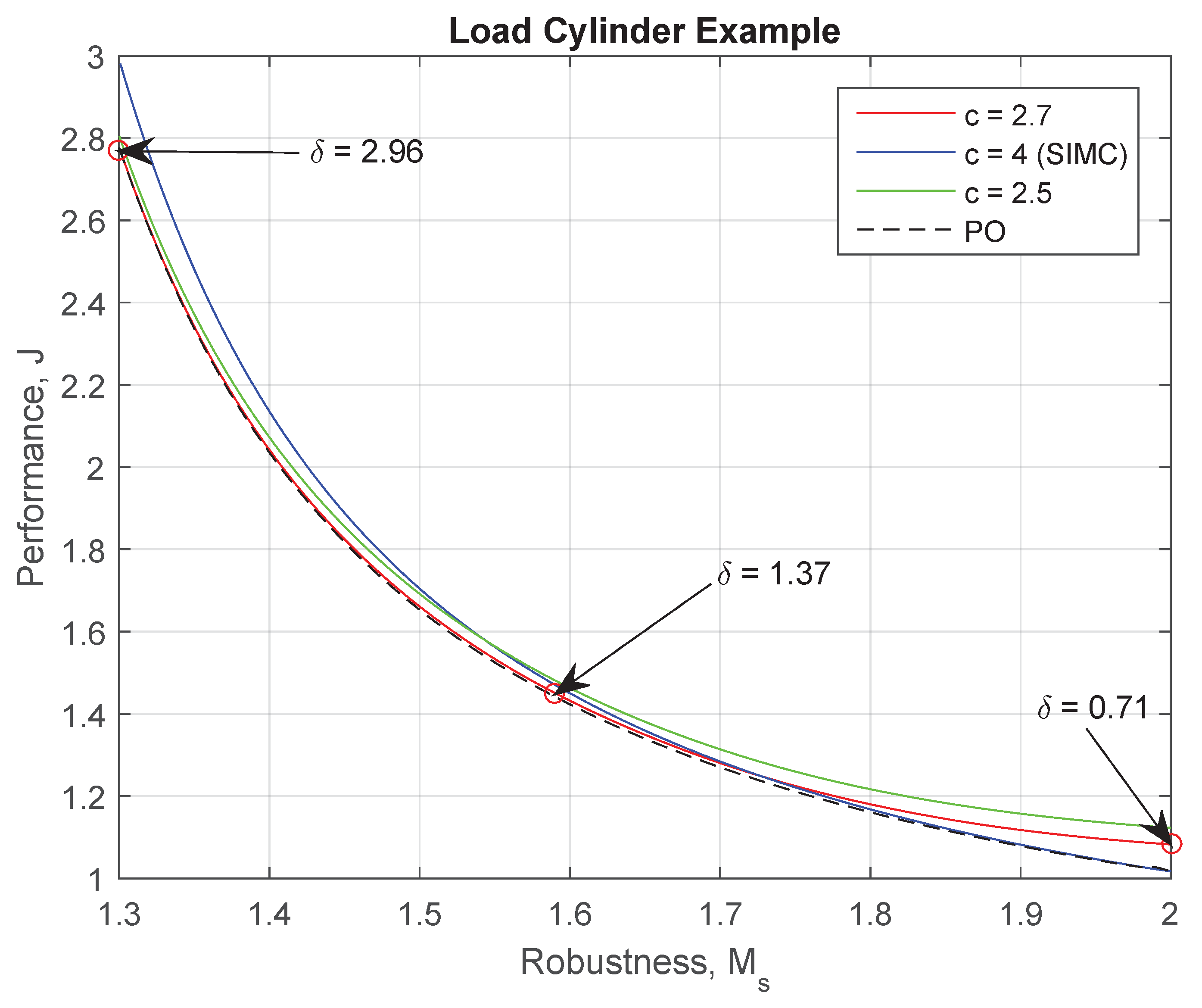
In this paper, we search for optimal MP parameters, i.e., choosing $\overline{c}$ which ensures the closed loop system some optimal robustness or performance setting, e.g., minimisation of the Integrated Absolute Error (IAE) or sensitivity index $M_s$ given a prescribed robustness. Figure 1 shows that $M_s$ is approximately minimised for $\overline{c}=2.0$. However, it might be argued that the changes in $M_s$ is negligible, and that $M_s$ is optimal over the MP parameter interval $1.5\le \overline{c}\le 4.0$.

Figure 1. Consider PI control of the FOPTD process model, $H_p\left(s\right)=\frac{e^{-s}}{s}$. The figure shows the robustness $M_s$ as a function of the MP parameter $\overline{c}$, given constant robustness, for the interval $1.5\le \overline{c}\le 4.0$.

It has been pointed out that there is usually a high degree of trial-and-error in choosing the closed loop time constant tuning parameter $T_c$ in SIMC and IMC (e.g., [1] for SIMC and [6] for IMC). Note that one also may focus on the maximum sensitivity peak $M_s$ of the sensitivity function as described in [14], where some inequalities relating to the Gain Margin (GM) and the Phase Margin (PM) to the robustness $M_s$ are proposed on p. 126. Consider that the values of the minimum robustness $M_s$ are in the interval $1.3\le M_s\le 2$ [14].

The contributions of this work are itemised in the incoming:

• The PI controller tuning method in the work of [1,2] is further developed with more optimal settings for the MP parameter as well as tuning for some special instance integrating systems.
• In the instance of a small or zero time delay $\tau =0$, we propose a variant in which the Maximum Time Delay Error (MTDE) $d{\tau }_{max}>0$ is the tuning parameter (see Section 3.2).
• Two optimal settings for the MP parameter are presented in Section 4. These are optimal in the sense that they minimise a Pareto performance objective (i.e., integrated absolute error for combined step changes in output and input disturbances) on two different aspects. One additional MP parameter is deduced from approximating the time delay with a (2, 1) Pade approximation in Section 3.3.
• Additional MP parameter settings are suggested for minimising a variety of given indices.
• The presented method (including variants of this) is demonstrated and compared to the Pareto-Optimal (PO) and SIMC (when possible) tuned PI controllers on various motivated (possible) higher order process model examples in Section 5.

The rest of this paper is organised as follows. The preliminary theory containing the definitions and some basic theory are given in Section 2. In Section 3, we present analytical results about the MTDE and present PI controller tuning rules as a function of a prescribed MTDE. Numerical simulation examples for some (possible) higher order systems/models are presented in Section 5. The conclusion and discussion remarks are given in Section 7.

2. Preliminary Theory

2.1. Definitions

Given a PI controller

$$\begin{array}{c}\hfill H_c\left(s\right)=K_p\frac{T_{i}s+1}{T_{i}s},\end{array}$$

(4)

where $K_p$ is the proportional constant and $T_i$ is the integral time constant.

Consider the standard feedback system with disturbances as illustrated in Figure 2. To compare the different controllers, we consider indices such as defined in [12,14,15]. Performance is measured in a feedback system by

$$\begin{array}{c}\hfill \mathrm{IAE}={\int }_0^{\infty }\left|e\right|dt.\end{array}$$

(5)

Figure 2. Consider a control feedback system where the plant model is described by the process model, $H_p\left(s\right)$, PI controller, $H_c\left(s\right)=K_p\frac{1+T_{i}s}{T_{i}s}$, and the disturbance model, $H_v\left(s\right)$, where disturbance v at the input when, $H_v\left(s\right)=H_p\left(s\right)$, and at the output when, $H_v\left(s\right)=1$. Input u, output y and reference r.

Furthermore, the following is defined.

• ${\mathrm{IAE}}_{vu}$ evaluates the performance in case of a step input disturbance ($H_v\left(s\right)=H_p\left(s\right)$), $v=1$ (default), with the reference, $r=0$.
• ${\mathrm{IAE}}_{vy}$ evaluates the performance in case of a step output disturbance ($H_v\left(s\right)=1$), $v=1$ (default), with the reference, $r=0$.
• ${\mathrm{IAE}}_r$ evaluates the performance in case of a reference unit step, $r=1$, with the disturbance, $v=0$.

Similarly, we define the Integrated Time-weighted Absolute Error (ITAE), Integrated Square Error (ISE) and Integrated Time-weighted Square Error (ITSE) and Total input Value (TV) as the following i.e.,

$$\begin{array}{ccc}\hfill \mathrm{ITAE}& =& {\int }_0^{\infty }t\left|e\right|dt,\hfill \end{array}$$

(6)

$$\begin{array}{ccc}\hfill \mathrm{ISE}& =& {\int }_0^{\infty }{e}^{2}dt,\hfill \end{array}$$

(7)

$$\begin{array}{ccc}\hfill \mathrm{ITSE}& =& {\int }_0^{\infty }t{e}^{2}dt,\hfill \end{array}$$

(8)

$$\begin{array}{ccc}\hfill \mathrm{TV}& =& {\int }_0^{\infty }|\Delta u_k|dt,\hfill \end{array}$$

(9)

where $\Delta u_k=u_k-u_{k-1}$.

Robustness is quantified according to the maximum sensitivity peak

$$\begin{array}{ccc}\hfill M_s& =& \underset{0\le \omega <\infty }{max}\left|S\left(j\omega \right)\right|={\left|\right|S\left(j\omega \right)\left|\right|}_{\infty },\hfill \end{array}$$

(10)

where, $S\left(j\omega \right)=\frac{1}{1+H_p\left(j\omega \right)H_c\left(j\omega \right)}$, and $\left|\right|·{\left|\right|}_{\infty }$ is the ${\mathcal{H}}_{\infty }$-norm.

2.2. Lag-Dominant Systems

Given a system approximated with a FOPTD model

$$\begin{array}{c}\hfill H_p\left(s\right)=\frac{K}{1+Ts}{e}^{-\tau s},\end{array}$$

(11)

where K is the process gain, $\tau$ is the time delay and T is the time constant. The system in Equation (11) may be defined as lag-dominant when $T>\tau$ which is the instance for numerous systems. It is known that, when $T\gg \tau$ then Equation (11) may be approximated with an IPTD model (see [6,7]). From Equation (11), we write,

$$\begin{array}{c}\hfill H_p\left(s\right)=\frac{K}{T}\frac{1}{s+\frac{1}{T}}{e}^{-\tau s}.\end{array}$$

(12)

Hence, when the system is lag-dominant and T “large”, we may approximate Equation (12) as an IPTD system (Equation (1)) where $k=\frac{K}{T}$ is the gain velocity (slope) and $\tau$ the time delay.

2.3. SIMC Tuning Rules

Given the FOPTD process in Equation (11). The standard SIMC PI controller settings [8,12,13] are as follows,

$$\begin{array}{c}\hfill K_p=\frac{T}{K(T_c+\tau )},T_i=min(T,4(T_c+\tau )),\end{array}$$

(13)

where $T_c$ is the prescribed time constant for the reference response chosen as $-\tau <T_c<\infty$.

Similarly, for an IPTD process as in Equation (1), we have the following PI controller settings,

$$\begin{array}{c}\hfill K_p=\frac{1}{k(T_c+\tau )},T_i=4(T_c+\tau ).\end{array}$$

(14)

3. Tuning for Maximum Time Delay Error

To get some understanding of the PM of the closed loop system and the MTDE, $d{\tau }_{max}$, we work out some analytic results in the following, which give a PI controller tuning method for IPTD processes.

3.1. Integrator Plus Time Delay Process

Consider an IPTD system where k is the gain velocity and $\tau$ is the time delay, and a PI controller. The loop transfer function, $H_0\left(s\right)=H_c\left(s\right)H_p\left(s\right)$, is

$$\begin{array}{c}\hfill H_0\left(s\right)=K_p\frac{1+T_{i}s}{T_{i}s}k\frac{e^{-\tau s}}{s}.\end{array}$$

(15)

The frequency response is given by $H_0\left(j\omega \right)=\left|H_0\left(j\omega \right)\right|e^{j\angle H_0\left(j\omega \right)}$, where the magnitude is $|H_0\left(j\omega \right)|=\frac{K_{p}k}{T_i{\omega }^2}\sqrt{1+{\left(T_i\omega \right)}^2}$ and the phase angle is $\angle H_0\left(j\omega \right)=-\tau \omega -\pi +arctan\left(T_i\omega \right)$. We obtain the gain crossover frequency ${\omega }_c$ analytically as $|H_0{\left(j\omega \right)}_c|=1$. From this, we obtain analytically that $\mathrm{PM}=\angle H_0\left(j{\omega }_c\right)+\pi$, and the MTDE $d{\tau }_{\max }$, such that, $0=\mathrm{PM}-d{\tau }_{\max }{\omega }_c$.

A factor f is defined as

$$\begin{array}{c}\hfill f=\frac{1+\sqrt{1+\frac{4}{{\left(K_p{T}_{i}k\right)}^2}}}{2}=\frac{1+\sqrt{1+\frac{4}{{\left(\alpha \beta \right)}^2}}}{2}.\end{array}$$

(16)

The gain crossover frequency is analytically given by

$$\begin{array}{c}\hfill {\omega }_c=\sqrt{f}{K}_{p}k.\end{array}$$

(17)

See previous paper [1] for proof of Equation (17).

The gain crossover frequency is then given by ${\omega }_c=\sqrt{f}\frac{\alpha }{\tau }$. We obtain the PM analytically as $\mathrm{PM}=-\sqrt{f}\alpha +arctan\left(\sqrt{f}\alpha \beta \right)$, and the MTDE as $d{\tau }_{\max }=\frac{\mathrm{PM}}{{\omega }_c}=\delta \tau$, where $\delta$ is defined as

$$\begin{array}{c}\hfill \delta =\frac{-\sqrt{f}\alpha +arctan\left(\sqrt{f}\alpha \beta \right)}{\sqrt{f}\alpha }=\frac{arctan\left(\sqrt{f}\alpha \beta \right)}{\sqrt{f}\alpha }-1.\end{array}$$

(18)

Consider the instance in which the MP parameter $\overline{c}=\alpha \beta$ is constant, then Equation (18) may be written as, $\delta =a\frac{1}{\alpha }-1$, and, $\delta =\frac{a}{\overline{c}}\beta -1$, where

$$\begin{array}{c}\hfill a=\frac{arctan\left(\sqrt{f}\alpha \beta \right)}{\sqrt{f}},\end{array}$$

(19)

is a function of $\overline{c}=\alpha \beta$ and constant. Notice that the parameter f is defined by Equation (16).

We have the following Algorithm 1.

Algorithm 1

(Max time delay error tuning).

The MP parameter is defined as

$$\begin{array}{c}\hfill \overline{c}=\alpha \beta .\end{array}$$

(20)

We express β as a linear function of a prescribed Relative Time Delay Error (RTDE) $\delta >0$, to ensure stability of the closed loop system. We have

$$\begin{array}{c}\hfill \beta =\frac{\overline{c}}{a}(\delta +1),\end{array}$$

(21)

where parameter a is given by Equation (19). Note that α can be expressed by

$$\begin{array}{c}\hfill \alpha =\frac{\overline{c}}{\beta }=\frac{a}{\delta +1}.\end{array}$$

(22)

or with regard to the PI controller parameters

$$\begin{array}{c}\hfill T_i=\frac{\overline{c}}{a}\left(\delta +1\right)\tau ,\end{array}$$

(23)

$$\begin{array}{c}\hfill K_p=\frac{a}{k\tau (\delta +1)}.\end{array}$$

(24)

Note that Algorithm 1 is written as a MATLAB m-file function given in Appendix C in a previous paper [1].

Before advancing, we demonstrate the above algorithm in an instance to enhance the robustness of the classical closed loop ZN PI controller tuning.

Example 1

(ZN with increased margins).

Given the classical ZN PI controller tuning (closed loop method), in which $\alpha =\frac{\pi }{4.4}$, $\beta =\frac{4}{1.2}$, where the RTDE $\frac{d{\tau }_{max}}{\tau }=\delta \approx 0.56$ and the robustness $M_s\approx 2.86$.

For the original ZN method, we have the MP parameter $\overline{c}=2.38$. Specifying an RTDE parameter, $\delta =\frac{d{\tau }_{max}}{\tau }=1.6$. Using Equations (21) and (22) gives the altered ZN PI controller parameters

$$\begin{array}{c}\hfill \alpha =0.42,\beta =5.55.\end{array}$$

(25)

The altered ZN PI controller tuning, $K_p=\frac{\alpha }{k\tau }$ and $T_i=\beta \tau$, for an IPTD process has margins $GM=3.35$, robustness $M_s=1.66$ and prescribed $\frac{d{\tau }_{max}}{\tau }=1.6$. The altered ZN PI controller tuning has relatively smooth closed loop responses with a relative damping slightly less than one. The ZN method parameter $\overline{c}=2.38$ is not too far from one of the recommended optimal parameters (see below).

Arguably, the most important characteristic of a PI controller setting is the robustness vs. model uncertainty in connection with a reasonably smooth and fast closed loop reference and disturbance responses. An MTDE $d{\tau }_{max}=1.6\tau$ is reasonable. This is approximately equal to the MTDE for the SIMC setting, $d{\tau }_{max}=1.59\tau$. One idea may be to find theoretical arguments for setting the MP parameter $\overline{c}$ such that the closed loop system gets some optimal settings, e.g., minimise the robustness $M_s$ given prescribed robustness $\delta$. Consider using the PI controller tuning rules deduced in [1] which gives the MP parameter $\overline{c}=2.76$.

The MP parameter $\overline{c}=\alpha \beta$ may be seen as a tuning parameter. SIMC uses a MP parameter $\overline{c}=4$ and the corresponding $GM\approx 2.96$, which is below the recommended margin, but the MTDE is acceptable, i.e., $d{\tau }_{max}=1.59\tau$. Based on the numerical simulations in this and previous works [1,2], we suggest a relatively broad interval for choosing the MP parameter $\overline{c}$, i.e., $\overline{c}\in [1.5,4.0]$.

Furthermore, we propose choosing the RTDE $\delta >0$ to unsure stability, and choosing $\delta$ as $\overline{c}\in [1.1,3.4]$ for robustness and to make certain that $1.3\le M_s\le 2.0$ (p. 125 in [14]) is reasonable.

3.2. Pure Integrating Process

Consider the limiting case of an integrating process, i.e., $\tau =0$ (no delay), or a time constant system with a large time constant such that $\frac{1}{T}\approx 0$, i.e., we consider a process model, $H_p\left(s\right)=\frac{k}{s}$. Using the definition for the RTDE tuning parameter, $\delta =\frac{d{\tau }_{\max }}{\tau }$, and the PI controller tuning Equations (23) and (24), we find the PI controller tuning

$$\begin{array}{c}\hfill T_i=\frac{\overline{c}}{a}\left(\frac{d{\tau }_{\max }}{\tau }+1\right)\tau =\frac{\overline{c}}{a}\left(d{\tau }_{\max }+\tau \right),\end{array}$$

(26)

$$\begin{array}{c}\hfill K_p=\frac{a}{k\tau (\frac{d{\tau }_{\max }}{\tau }+1)}=\frac{a}{k(d{\tau }_{\max }+\tau )}.\end{array}$$

(27)

Notice that Equations (26) and (27) are tuning variants in which the MTDE $d{\tau }_{\max }>0$ is the tuning parameter instead of the RTDE $\delta$.

Consider the limiting case of an integrating process, i.e., $\tau =0$ (no delay). From Equations (26) and (27), we find the PI controller tuning

$$\begin{array}{c}\hfill T_i=\frac{\overline{c}}{a}d{\tau }_{\max },\end{array}$$

(28)

$$\begin{array}{c}\hfill K_p=\frac{a}{kd{\tau }_{\max }}.\end{array}$$

(29)

Notice that $PM=a\sqrt{f}$ in this case.

3.3. Using a ($2,1$) Pade Approximation

Consider the disturbance response with PI control,

$$\begin{array}{ccc}\frac{y}{v}\left(s\right)\hfill & =\hfill & \frac{H_p}{1+H_c{H}_p}=\frac{k\frac{e^{-\tau s}}{s}}{1+K_p\frac{1+T_{i}s}{T_{i}s}k\frac{e^{-\tau s}}{s}}\hfill \\ & =\hfill & \frac{ks{e}^{-\tau s}}{s^2+\frac{K_{p}k}{T_i}(1+T_{i}s)e^{-\tau s}}.\hfill \end{array}$$

(30)

Consider a ($2,1$) Pade approximation, $e^x=\frac{6+4x+x^2}{6-2x}$, i.e., with a second order numerator polynomial and a first order denominator polynomial, i.e., an approximation,

$$\begin{array}{c}\hfill e^{-\tau s}\approx \frac{1-b_{1}s+b_2{s}^2}{1+a_{1}s},\end{array}$$

(31)

where $a_1=\frac{\tau }{3}$, $b_1=\frac{2\tau }{3}$ and $b_2=\frac{{\tau }^2}{6}$.

Using the same procedure as in Section 5.2 in [1], and with unit relative damping, we find a third order polynomial for the closed loop response,

$$\begin{array}{c}\hfill \frac{y}{v}\left(s\right)=\frac{T_{i}s}{K_p}\frac{b_2{s}^2-b_{1}s+1}{(\frac{a_1{T}_i}{k{K}_p}+b_2{T}_i)s^3+(b_2-b_1{T}_i+\frac{T_i}{k{K}_p})s^2+(T_i-b_1)s+1}.\end{array}$$

(32)

We prescribe a third order polynomial

$$\begin{array}{ccc}\Pi \left(s\right)\hfill & =\hfill & (1-{\tau }_{0}s)({\tau }_0^2{s}^2+2{\tau }_{0}s+1)={(1+{\tau }_{0}s)}^3\hfill \\ & =\hfill & {\tau }_0^3{s}^3+3{\tau }_0^2{s}^2+3{\tau }_{0}s+1.\hfill \end{array}$$

(33)

When comparing Equations (32) and (33), we find that

$$\begin{array}{ccc}\hfill {\tau }_0^3& =& T_i(\frac{a_1}{k{K}_p}+b_2),\hfill \end{array}$$

(34)

$$\begin{array}{ccc}\hfill 3{\tau }_0^2& =& b_2-T_i(b_1-\frac{1}{k{K}_p}),\hfill \end{array}$$

(35)

$$\begin{array}{ccc}\hfill 3{\tau }_0& =& T_i-b_1.\hfill \end{array}$$

(36)

By inserting Equations (34) and (36) into Equation (35), it can be shown that

$$\begin{array}{c}\hfill {\left(\frac{{\tau }_0}{\tau }\right)}^3-{\left(\frac{{\tau }_0}{\tau }\right)}^2-\frac{7}{6}\left(\frac{{\tau }_0}{\tau }\right)-\frac{11}{54}=0.\end{array}$$

(37)

We solve the third order polynomial in Equation (37) with respect to $\frac{{\tau }_0}{\tau }$, and find a real positive solution, $\frac{{\tau }_0}{\tau }\approx 1.7385$.

Furthermore, we find that the PI controller parameters

$$\begin{array}{c}\hfill T_i=3{\tau }_0+b_1,K_p=\frac{a_1{T}_i}{k({\tau }_0^3-b_2{T}_i)},\end{array}$$

(38)

where ${\tau }_0$ may be seen as a tuning parameter.

When assuming that the response time constant ${\tau }_0=c\tau$, then we may express the PI controller parameters $K_p=\frac{\alpha }{k\tau }$ and $T_i=\beta \tau$ with

$$\begin{array}{ccc}\hfill \beta & =& \frac{9c+2}{3}=3c+\frac{2}{3},\hfill \end{array}$$

(39)

$$\begin{array}{ccc}\hfill \alpha & =& \frac{2(9c+2)}{18c^3-9c-2}=\frac{c+\frac{2}{9}}{c^3-\frac{1}{2}c-\frac{1}{9}},\hfill \end{array}$$

(40)

where the product $\overline{c}=\alpha \beta$ is a nonlinear function of the tuning parameter c. We find that it makes sense to choose c in the interval, $1.4\le c\le 2.5$.

From the PI controller setting in Equation (38) with ${\tau }_0=1.7385$, we find the MP parameter $\overline{c}=\alpha \beta =K_{p}k{T}_i\approx 2.6985$.

For reducing the complexity of the problem, the (1, 2) Pade approximation was used; e.g., a (2, 2) Pade would result in a fourth order polynomial. Notice that a (1, 1) Pade approximation was used in the earlier work of [1] in Section 5.2.

4. Optimal Performance Settings

Consider the following Pareto performance objective defined as

$$\begin{array}{c}\hfill J\left(p\right)=s_r\frac{{\mathrm{IAE}}_x\left(p\right)}{{\mathrm{IAE}}_x^o}+(1-s_r)\frac{{\mathrm{IAE}}_{vu}\left(p\right)}{{\mathrm{IAE}}_{vu}^o},\end{array}$$

(41)

where $s_r$ is the servo-regulator parameter originally introduced in [2], and is chosen in the interval $0\le s_r\le 1.0$ for the weighting between output disturbance (servo) weighting $s_r=1.0$ and input disturbance (regulator) weighting $s_r=0$. In Equation (41), the function argument is $p={[K_p,T_i]}^T$. In this work, we set $s_r=0.5$ ([16]). Furthermore, we set $x=vy$, which was argued in [17] to be the equivalent of setting $x=r$, which was used in the original work of [16] and also [2]. The reference/weight values are calculated as following, ${\mathrm{IAE}}_{vy}^o={min}_p{\mathrm{IAE}}_{vy}\left(p\right)$, and, ${\mathrm{IAE}}_{vu}^o={min}_p{\mathrm{IAE}}_{vu}\left(p\right)$, for a prescribed robustness $M_s^{pre}$. We set $M_s^{pre}=1.59$ which is the robustness value corresponding to a SIMC-tuned PI controller with $T_c=\tau$ for a FOPTD process where $K=T=\tau =1$ ([16]).

We consider the reference example where we are given an IPTD process with $k=\tau =1$. We find the same reference values as in [18], viz. ${\mathrm{IAE}}_{vy}^o=2.17$ where $K_p=0.5$ and $T_i=\infty$, and ${\mathrm{IAE}}_{vu}^o=15.10$ where $T_i=5.8$ and $K_p=0.4$.

The following main performance objective is defined in a mean square error sense,

$$\begin{array}{c}\hfill V_M(x,y)=\frac{1}{M}\sum _{i=1}^M{(J_x\left(i\right)-J_y\left(i\right))}^2,\end{array}$$

(42)

where x is a tuning method and, $y=\mathrm{PO}$ (default) and M = length($M_s$).

A couple of optimal suggestions for the choice of the MP parameter are worked out in the following. The first MP parameter setting may be found by solving the following optimization problem,

$$\begin{array}{ccc}\hfill \overline{c}& =& arg\underset{\overline{c}}{min}{V}_M(\mathrm{Alg}.1\left(\overline{c}\right),\mathrm{Alg}.1^o)=2.7,\hfill \end{array}$$

(43)

where Alg. 1 ($\overline{c},{\delta }_i$) and Alg. 1^o (${\delta }_i$) is pre-calculated as follows

$$\begin{array}{c}\hfill J_{\mathrm{Alg}.1_i}=\underset{\overline{c}}{min}{J}_{\mathrm{Alg}.1}(\overline{c},{\delta }_i)\forall 1.1\le {\delta }_i\le 3.4.\end{array}$$

(44)

Interestingly, the MP parameter setting in Equation (43) is approximately equal to the setting which is deduced in Section 3.3. Additional MP parameter settings are given in Table 1 based on solving Equation (43) for different servo-regulator parameters $0\le s_r\le 1.0$ in the Pareto performance objective J (Equation (41)).

The second MP parameter is found by

$$\begin{array}{c}\hfill \overline{c}=arg\underset{\overline{c}}{min}{V}_M(\mathrm{Alg}.1\left(\overline{c}\right),\mathrm{PO})=2.5,\end{array}$$

(45)

where Alg. 1 ($\overline{c},\delta \left(M_s^i\right)$) and PO ($M_s^i$) are pre-calculated as follows

$$\begin{array}{c}\hfill J_{P{O}_i}=\underset{p}{min}J(p,M_s^i)\forall 1.1\le M_s^i\le 3.4.\end{array}$$

(46)

Notice that $\overline{c}=2.5$ is equal to the recommended MP parameter in [2]. However, the MP parameter in this paper results from an optimization problem, while the one proposed in [2] originated from an ad hoc approach.

Figure 3 illustrates the two MP parameters described above. In terms of the main performance objective $V_M$ (Equation (42)), Table 2 shows that $\overline{c}=2.5$ is $\frac{V_{\overline{c}=4}}{V_{\overline{c}=2.5}}=3e+4$ times better than SIMC (arguably $\overline{c}=4$), and $\frac{V_{\overline{c}=2.7}}{V_{\overline{c}=2.5}}=78$ times better than $\overline{c}=2.7$.

Figure 3. Reference example (Example 2). Consider PI control of the IPTD model, $H_p\left(s\right)=\frac{e^{-s}}{s}$. The figure illustrates the trade-off between the Pareto performance objective J (Equation (41)) and robustness $M_s$ (Equation (10)). It illustrates the MP parameters $\overline{c}=2.5$ and $\overline{c}=2.7$ for Algorithm 1 proposed in Section 4. SIMC is added for comparison.

Table 2. Reference example (Example 2), i.e., an IPTD model, $H_p\left(s\right)=\frac{e^{-s}}{s}$. Comparing the different settings for the MP parameters for Algorithm 1 and SIMC using the main performance objective $V_M$ (Equation (42)).

Method	$\overline{\mathit{c}}$ = 2.5	$\overline{\mathit{c}}$ = 2.7	SIMC
$V_M$/e-4	0.02	1.56	592.75

Based on numerical simulations, we present the recommended settings for choosing the MP parameter $\overline{c}$ as proposed in Table 3.

Table 3. Summary: The table shows the recommended settings for the MP parameter $\overline{c}$ for minimizing the objectives in the first row.

	${\mathit{M}}_{\mathit{s}}$	${\mathbf{IAE}}_{\mathit{vu}}$	${\mathbf{ITAE}}_{\mathit{vu}}$	${\mathbf{ITAE}}_{\mathit{r}}$	${\mathbf{IAE}}_{\mathit{r}}$	${\mathit{V}}_{\mathit{M}}(\mathit{\delta }\mathit{O})$	${\mathit{V}}_{\mathit{M}}\left(\mathit{t}\right)$
$\overline{c}$	2.0	2.4	2.4	2.6	4.0	2.7	2.5

Consider PI controller settings for an IPTD system, $H_p\left(s\right)=k\frac{e^{-\tau s}}{s}$, with varying gain velocity, k, and time delay $\tau \ge 0$. Table 4 and Table 5 illustrate the ${\overline{c}}_{min}={argmin}_{\overline{c}}{M}_s$, i.e., the minimum of $M_s$, ${\mathrm{IAE}}_{vu}$, $\mathrm{ITAE}$, ${\mathrm{ITAE}}_{vu}$ and ${\mathrm{IAE}}_r$, $\mathrm{TV}$, $\mathrm{ISE}$, $\mathrm{ITSE}$, ${\mathrm{ITAE}}_r$, respectively, as a function of $\overline{c}$.

Table 4. Consider PI controller settings for an IPTD system, $H_p\left(s\right)=k\frac{e^{-\tau s}}{s}$, with varying gain velocity, k, and time delay $\tau \ge 0$. The table illustrates the ${\overline{c}}_{\min }={\arg \min }_{\overline{c}}{M}_s$, i.e., the minimum of the $M_s$, ${\mathrm{IAE}}_{vu}$, $\mathrm{ITAE}$ and ${\mathrm{ITAE}}_{vu}$ indices as a function of $\overline{c}$, with PI controller settings from Algorithm 1.

k	$\mathit{\tau }$	${\mathit{M}}_{\mathit{s}}$	${\mathbf{IAE}}_{\mathit{vu}}$	$\mathbf{ITAE}$	${\mathbf{ITAE}}_{\mathit{vu}}$
1	0.1	2.0	2.45	2.45	2.45
1	0.3	2.0	2.4	2.45	2.4
1	0.5	2.0	2.4	2.45	2.4
1	1	2.0	2.4	2.4	2.4
1	2	2.0	2.4	2.4	2.4
1	4	2.0	2.4	2.4	2.4
0.1	1	2.0	2.4	2.5	2.4
0.1	2	2.0	2.4	2.45	2.4
0.1	4	2.0	2.4	2.45	2.4

Table 5. Consider PI controller settings for an IPTD system, $H_p\left(s\right)=k\frac{e^{-\tau s}}{s}$, with varying gain velocity, k, and time delay $\tau \ge 0$. The table illustrates ${\overline{c}}_{\min }={\arg \min in}_{\overline{c}}{M}_s$, i.e., the minimum of ${\mathrm{IAE}}_r$, $\mathrm{Tv}$, $\mathrm{ISE}$, ${\mathrm{ITAE}}_r$ and $\mathrm{ITSE}$ indices as a function of $\overline{c}$, with PI controller settings from Algorithm 1.

k	$\mathit{\tau }$	${\mathbf{ITAE}}_{\mathit{r}}$	$\mathbf{ITSE}$	$\mathbf{ISE}$	$\mathbf{TV}$	${\mathbf{IAE}}_{\mathit{r}}$
1.0	0.1	2.7	3.4	4.0	4.0	4.0
1.0	0.3	2.7	3.2	4.0	4.0	4.0
1.0	0.5	2.7	3.1	3.5	4.0	4.0
1.0	1.0	2.6	3.1	3.2	4.0	4.0
1.0	2.0	2.6	3.0	3.1	4.0	4.0
1.0	4.0	2.6	3.0	3.1	4.0	4.0
0.1	1.0	2.6	3.9	4.0	4.0	4.0
0.1	2.0	2.6	3.2	4.0	4.0	4.0
0.1	4.0	2.6	3.1	3.6	4.0	4.0

Consider PI controller settings for an IPTD system, $H_p\left(s\right)=k\frac{e^{-\tau s}}{s}$, where $k=1$ and time delay $\tau =1$. Figure 4 shows the indices $M_s$, ${\mathrm{ITAE}}_{vu}$, ${\mathrm{IAE}}_r$, ${\mathrm{ITAE}}_r$, ${\mathrm{IAE}}_r$, $\mathrm{TV}$, $\mathrm{ISE}$, ${\mathrm{ITAE}}_{vu}$ and $\mathrm{IAE}$ as a function of varying the MP parameter $\overline{c}\in [1.5,4.0]$ and with prescribed RTDE $\delta =1.6$.

Figure 4. Consider PI control of an IPTD process, $H_p\left(s\right)=k\frac{e^{-\tau s}}{s}$ with process parameters $k=1$ and $\tau =1$. PI controller $H_c\left(s\right)=K_p\frac{1+T_{i}s}{T_{i}s}$ with settings as in Algorithm 1. The figure shows the indices $M_s$, ${\mathrm{ITAE}}_{vu}$, ${\mathrm{IAE}}_r$, ${\mathrm{ITAE}}_r$, ${\mathrm{IAE}}_r$, $\mathrm{TV}$, $\mathrm{ISE}$, ${\mathrm{ITAE}}_{vu}$ and $\mathrm{IAE}$ as a function of varying the MP parameter $\overline{c}\in [1.5,4.0]$ and with prescribed RTDE $\delta =1.6$.

5. Simulation Examples

In the following simulations (if possible), we compare Algorithm 1, with the recommended MP parameter settings, vs. the SIMC tuning rule [12].

We continue with studying the reference example considered in Section 4. See also [1] for additional details on this example.

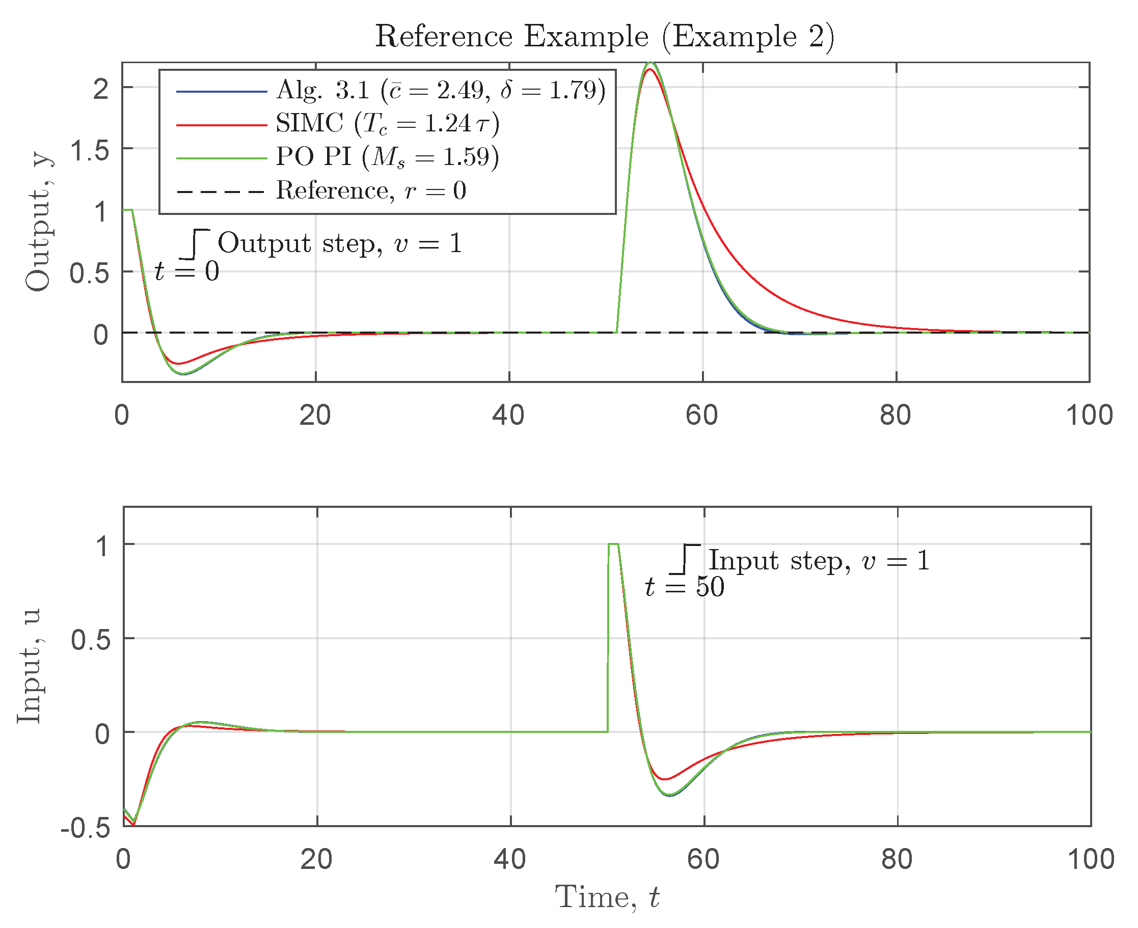
Example 2

(Reference Example).

The same IPTD example as in [1] is used, i.e., a process model, $H_p\left(s\right)=k\frac{e^{-\tau s}}{s}$, with gain velocity $k=1$ and time delay $\tau =1$ is considered.

The time-domain responses given a prescribed robustness, $M_s=1.59$, are illustrated in Figure 5. The corresponding PI controller parameters, indices and margins are given in Table 6. The margins for the controllers are all acceptable, i.e., $GM>2$ and $PM>30$ as in [14].

Figure 5. Example 2 (Reference example). Consider PI control of an IPTD process model, $H_p\left(s\right)=\frac{e^{-s}}{s}$. The figure illustrates the time-domain responses, given a prescribed robustness $M_s=1.59$, of the following methods: the PO PI, SIMC with prescribed closed loop time constant $T_c=1.24\tau$ and Algorithm 1 where the MP parameter $\overline{c}=2.5$ (proposed in Section 4) and RTDE $\delta =1.79$. An output disturbance unit step is presented at time $t=0$ and an input disturbance unit step at time $t=50$.

Table 6. Example 2. Consider PI control of the IPTD process model, $H_p\left(s\right)=\frac{e^{-s}}{s}$. The table shows the controller parameter, indices and margins are given for prescribed robustness $M_s=1.59$ for the following methods: Alg. 1 ($\overline{c}=2.5,\delta =1.79$), SIMC ($T_c=1.24\tau$) and PO PI ($M_s=1.59$).

	Alg. 1	SIMC	PO PI
$K_p$	0.41	0.45	0.41
$T_i$	6.14	8.96	6.28
${\mathrm{IAE}}_{vy}$	4.39	4.24	4.37
${\mathrm{IAE}}_{vu}$	15.26	20.06	15.39
J	1.52	1.64	1.52
TV	3.33	3.12	3.31
GM	3.56	3.34	3.54
PM	44.57	50.02	44.94
DM	1.79	1.90	1.80
$M_s$	1.59	1.59	1.59

Example 3

(Lag-dominant system).

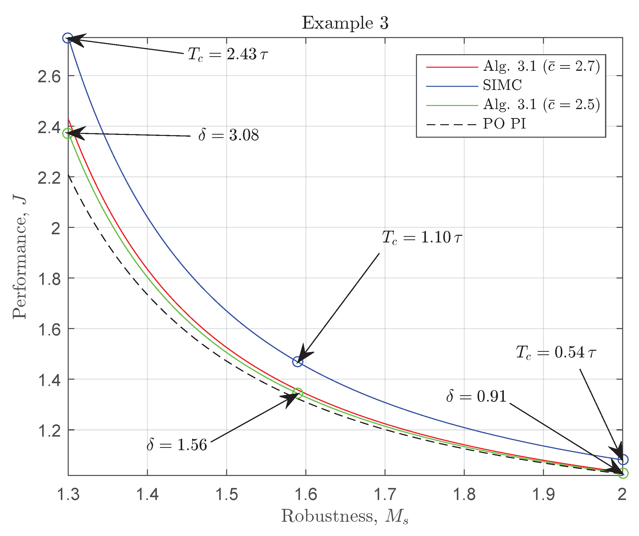
An air-heater was studied in [19] and it was found that a FOPTD model with process gain $K=5.7$, time delay $\tau =4$ and time constant $T=60$, gives a sufficient model approximation. We approximate the FOPTD model as an IPTD process where the gain velocity (slope) $k=\frac{K}{T}=0.095$ and time delay, $\tau =4$.

The Pareto performance objective J vs. $M_s$ trade-off curves are shown in Figure 6. In terms of the main performance objective $V_M$ it can be seen in Table 7 that $\overline{c}=2.5$ is $\frac{V_{\overline{c}=2.7}}{V_{\overline{c}=2.5}}=1.9$ times better than $\overline{c}=2.7$ and $\frac{V_{\mathrm{SIMC}}}{V_{\overline{c}=2.5}}=12.2$ times better than SIMC.

Figure 6. Example 3. Consider PI control of the FOPTD process model, $H_p\left(s\right)=K\frac{e^{-\tau s}}{Ts+1}$, where $K=5.7$, $\tau =4$ and $T=60$. The figure shows the trade-off curves with the Pareto performance objective J (Equation (41)) and robustness $M_s$ (Equation (10)). It illustrates the MP parameters $\overline{c}=2.5$ and $\overline{c}=2.7$ for Algorithm 1 (proposed in Section 4). SIMC with set-point time constant $T_c$ is added for comparison.

Table 7. Example 3. The table shows the comparison of the settings for Algorithm 1 and SIMC using the main performance objective $V_M$ (Equation (42)).

Method	$\overline{\mathit{c}}$ = 2.5	$\overline{\mathit{c}}$ = 2.7	SIMC
$V_M$/e-2	0.57	1.08	6.96

The time-domain responses, given a prescribed robustness, $M_s=1.59$, are illustrated in Figure 7. The corresponding PI controller parameters, indices and margins are given in Table 8. The margins for the controllers are all acceptable, i.e., $GM>2$ and $PM>30$ as in [14]. Notice, that the prescribed MTDE, $d{\tau }_{max}=\delta \tau =7.16$ is almost equal the exact $DM=7.51$.

Figure 7. Example 3. Consider PI control of the FOPTD process model, $H_p\left(s\right)=K\frac{e^{-\tau s}}{Ts+1}$, where $K=5.7$, $\tau =4$ and $T=60$. The figure illustrates the time-domain responses, given a prescribed robustness $M_s=1.59$, of the following methods: the PO PI, SIMC with prescribed closed loop time constant $T_c=1.10\tau$, and Algorithm 1 where the MP parameter $\overline{c}=2.5$ (proposed in Section 4) and RTDE $\delta =1.56$. An output disturbance unit step is presented at time $t=0$ and an input disturbance unit step at time $t=140$.

Table 8. Example 3. The table shows the PI controller parameter, indices and margins are given for prescribed robustness $M_s=1.59$.

	Alg. 1	SIMC	PO PI
$K_p$	1.17	1.25	1.12
$T_i$	22.55	33.60	19.47
${\mathrm{IAE}}_{vy}$	15.13	13.53	15.70
${\mathrm{IAE}}_{vu}$	17.73	25.16	15.89
J	1.39	1.52	1.37
TV	3.94	3.70	4.05
GM	3.36	3.22	3.46
PM	50.49	56.21	47.83
DM	7.51	8.08	7.26
$M_s$	1.59	1.59	1.59

Some results regarding a couple of motivated higher order processes are presented in the following examples. Notice that SIMC offers the half-rule model reduction technique. However, for our case, we approximate the higher order systems by identifying two parameters, the unit reaction rate $R_1$ and the lag L from a step response, i.e., the Process–Reaction Curve (PRC) as presented in the work of ZN [9,10,11]. We denote the variant as follows: PRC + Algorithm 1.

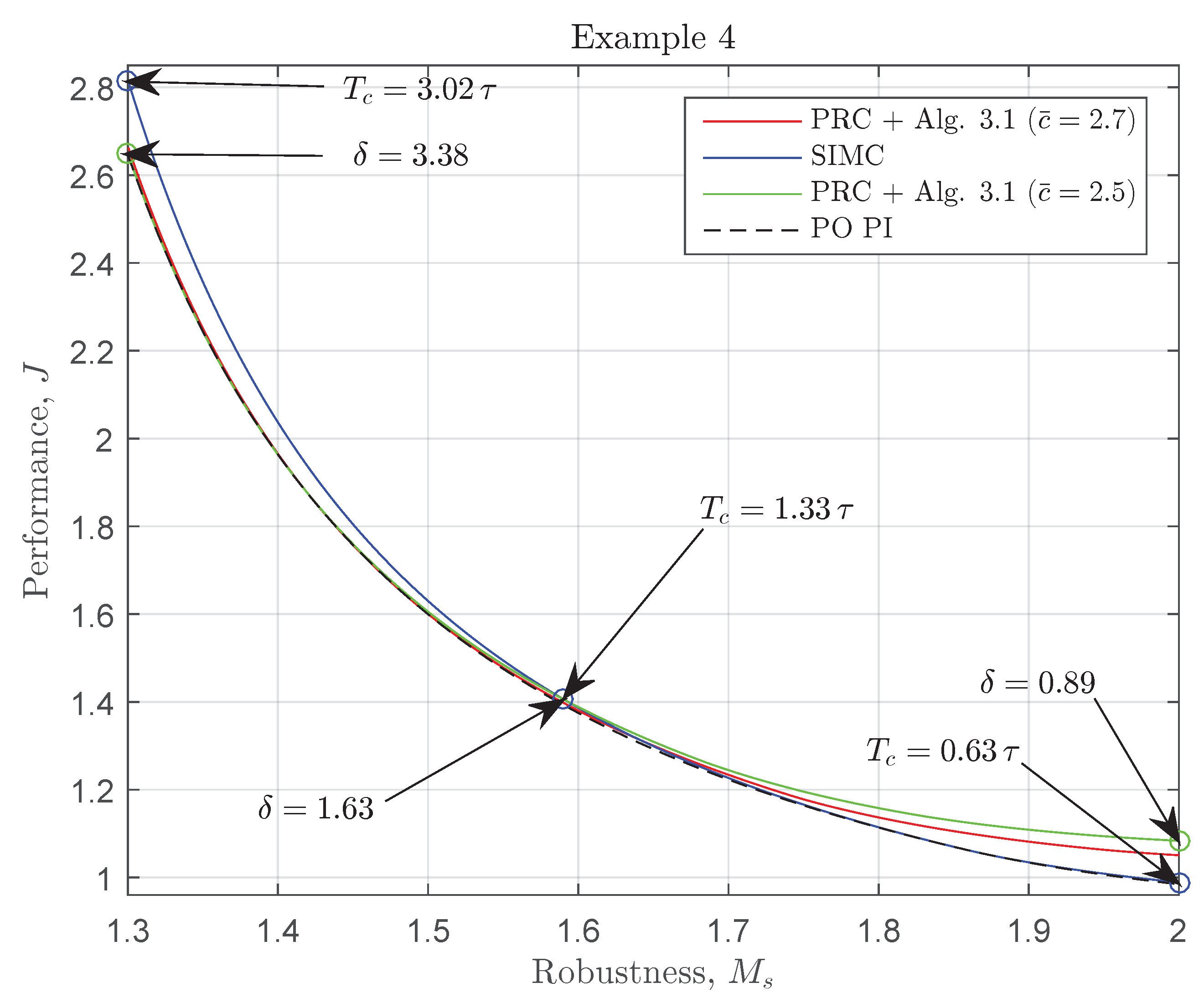
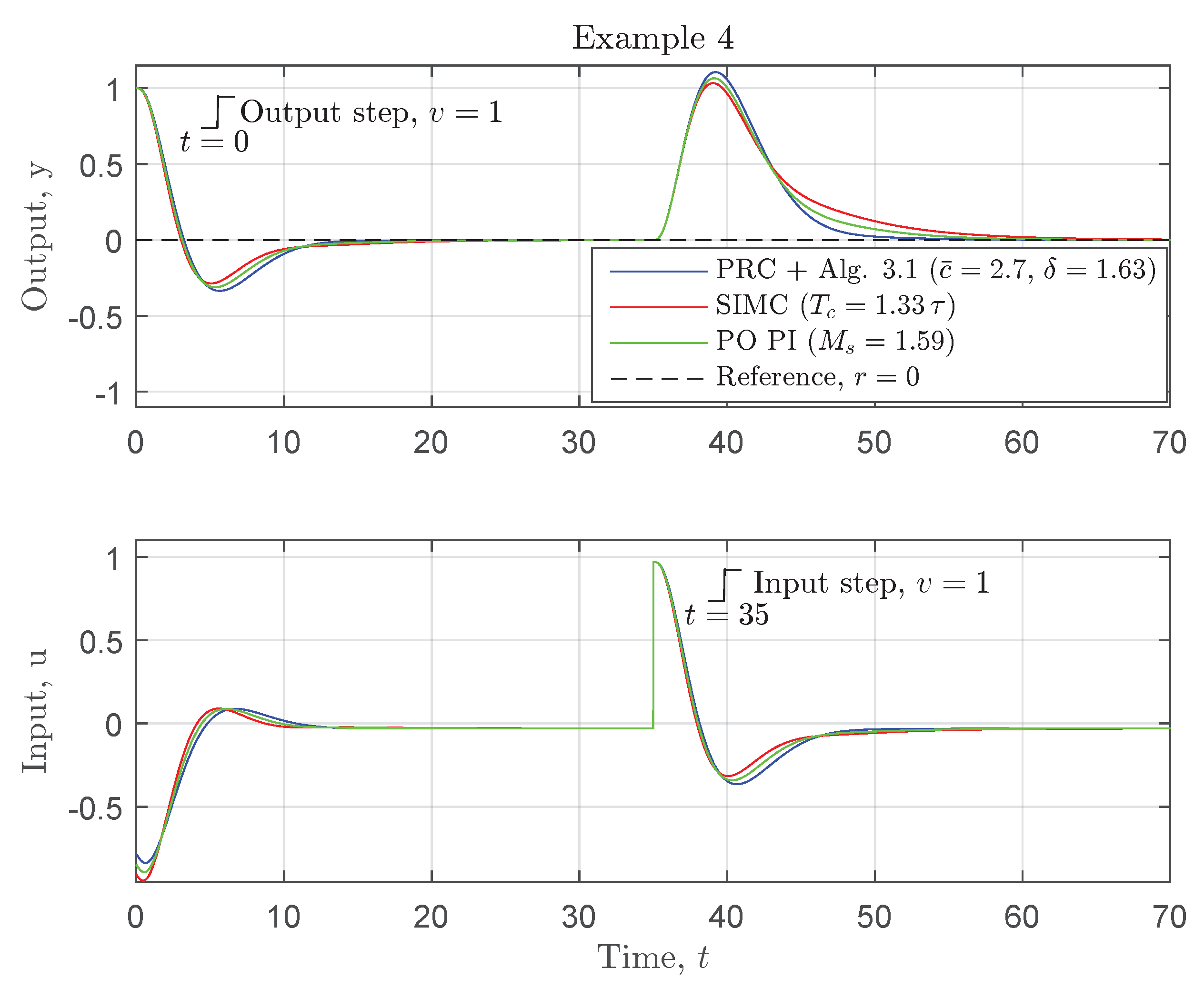
Example 4

(Higher order process).

A distillation column studied in [20] (p. 591) is partly described by the following process model,

$$\begin{array}{c}\hfill H_p\left(s\right)=\frac{34}{(54s+1){(0.5s+1)}^2}.\end{array}$$

(47)

By identifying the lag L and the maximum slope (unit reaction rate) $R_1$ from the PRC method we may approximate the process model as an IPTD model with gain velocity $k=R_1=0.597$ and time delay $\tau =L=0.923$.

Using the half-rule technique in SIMC, we approximate a FOPTD model where the gain $K=34$, time constant $T=54+\frac{0.5}{2}=54.25$, and time delay $\tau =0.5+\frac{0.5}{2}=0.75$.

The Pareto Performance objective J vs. robustness $M_s$ trade-off curves are illustrated in Figure 8. Notice, that $\overline{c}=2.7$ is the closest to optimal on the most robust part of the $M_s$-interval. SIMC is crossing $\overline{c}=2.7$ around $M_s=1.64$ and is the closest to optimal on the less robust part. In terms of the main performance objective $V_M$, we show in Table 9 that $\overline{c}=2.7$ is $\frac{V_{\overline{c}=2.5}}{V_{\overline{c}=2.7}}=2.3$ times better than $\overline{c}=2.5$, and $\frac{V_{\mathrm{SIMC}}}{V_{\overline{c}=2.7}}=20.7$ times better than SIMC.

Figure 8. Example 4. Consider PI control of the higher order process model (Equation (47)). The figure illustrates the trade-off curves with the Pareto performance objective J (Equation (41)) and robustness $M_s$ (Equation (10)). It shows the MP parameter settings $\overline{c}=2.5$ and $\overline{c}=2.7$ for Algorithm 1 proposed in Section 4. SIMC is added for comparison.

Table 9. Example 4. The table shows the comparison of the different settings for Algorithm 1 and SIMC using the main performance $V_M$ (Equation (42)).

Method	$\overline{\mathit{c}}$ = 2.5	$\overline{\mathit{c}}$ = 2.7	SIMC
$V_M$/e-3	0.7	0.3	6.2

The time-domain responses, for a prescribed robustness $M_s=1.59$, are illustrated in Figure 9. The corresponding PI controller parameters, indices and margins are given in Table 10. The margins for the controllers are all acceptable, i.e., $GM>2$ and $PM>30$, as in [14]. Notice, that the prescribed MTDE, $d{\tau }_{max}=\delta \tau =1.50$ is almost equal to the exact $DM=1.54$.

Figure 9. Example 4. Consider PI control of the higher order process model (Equation (47)). The figure illustrates the time-domain responses, given a prescribed robustness $M_s=1.59$, of the following methods: the PO PI controller vs. SIMC with closed loop time constant $T_c=1.33\tau$, and PRC + Algorithm 1 where the MP parameter setting $\overline{c}=2.7$ (proposed in Section 4) and RTDE $\delta =1.63$. An output disturbance unit step is presented at time $t=0$ and an input disturbance unit step at time $t=35$.

Table 10. Example 4. The table shows the PI controller parameters, indices and margins are given for prescribed robustness $M_s=1.59$.

	Alg. 1	SIMC	PO PI
$K_p$	0.78	0.91	0.85
$T_i$	5.35	7.04	6.06
${\mathrm{IAE}}_{vy}$	3.62	3.35	3.48
${\mathrm{IAE}}_{vu}$	6.83	7.74	7.14
J	1.41	1.41	1.39
TV	3.77	3.77	3.77
GM	6.74	6.13	6.39
PM	43.63	46.74	45.19
DM	1.54	1.49	1.51
$M_s$	1.59	1.59	1.59

Note that the half-rule technique in SIMC is not compatible with process models containing complex poles/underdamped dynamics, hence, in such cases, we consider arguably the same algorithm as SIMC, i.e., Algorithm 1, where the MP parameter, $\overline{c}=4$. An example of this is given in the following.

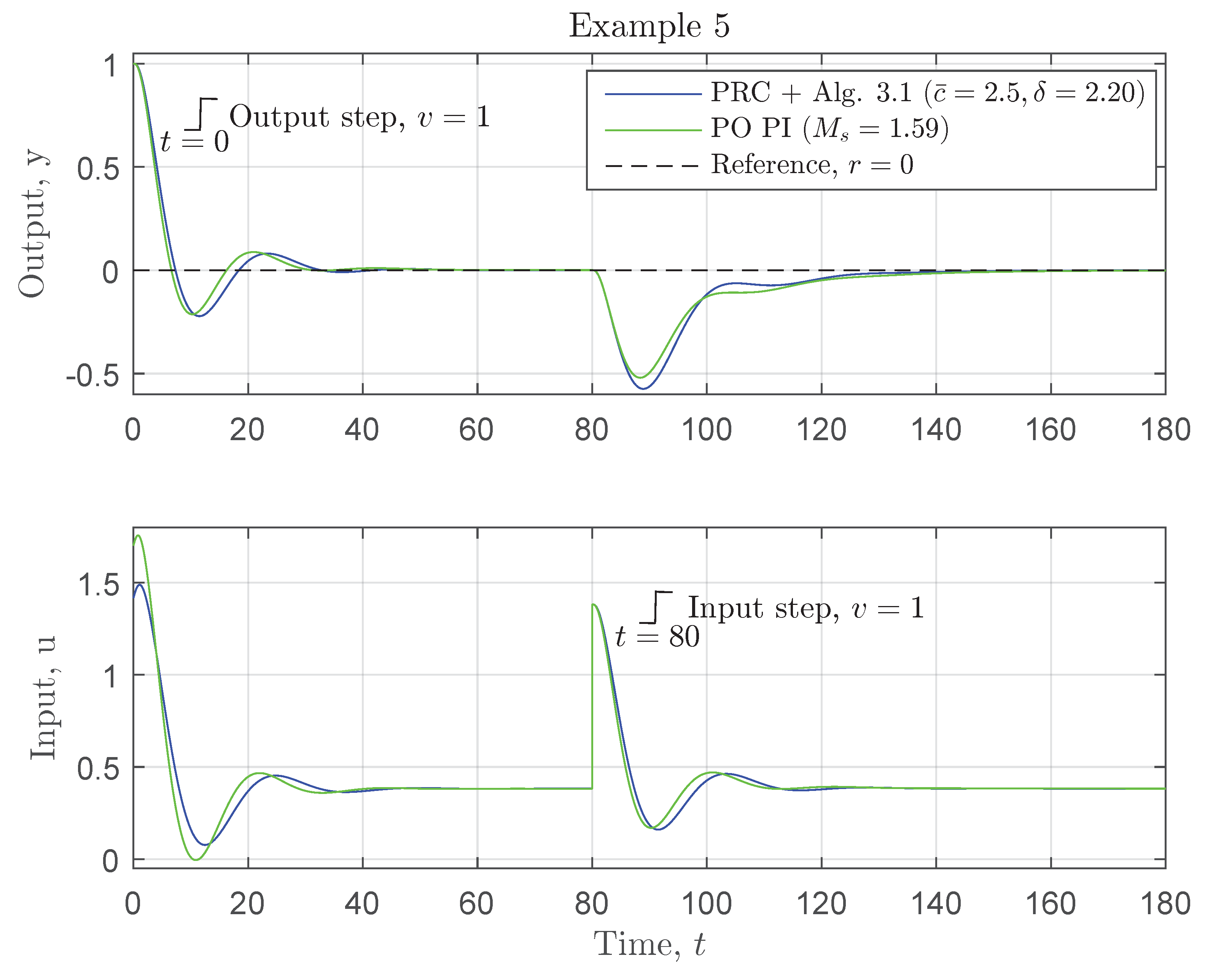
Example 5

(Underdamped system).

An unmanned submersible vehicle studied in [21] is described partly by

$$\begin{array}{ccc}\hfill H_p\left(s\right)& =& \frac{-2.6158(2.299s+1)}{(0.8131s+1)(0.5s+1)({\left(7.692s\right)}^2+1.738\left(7.692s\right)+1)},\hfill \end{array}$$

(48)

i.e., from commanded elevator deflection u to the pitch angle of the vehicle y. We approximate Equation (48) by an IPTD model with gain velocity $k=R_1=-0.145$ and time delay $\tau =L=1.729$.

The Pareto performance objective J vs. $M_s$ trade-off curves are illustrated in Figure 10. In terms of the main performance objective $V_M$, we show in Table 11 that $\overline{c}=2.5$ is $\frac{V_{\overline{c}=4}}{V_{\overline{c}=2.5}}=7.3$ times better than $\overline{c}=4$ and $\frac{V_{\overline{c}=2.7}}{V_{\overline{c}=2.5}}=1.3$ times better than $\overline{c}=2.7$. Notice that $\overline{c}=2.5$ is closest to optimal on the most robust part of the $M_s$-interval. Furthermore, $\overline{c}=4$ is seen crossing both $\overline{c}=2.5$ and $\overline{c}=2.7$ around $M_s=1.55$ and is closest to optimal on the less robust part.

Figure 10. Example 5. Consider PI control of the higher order underdamped process model (Equation (48)). The figure shows the trade-off curves with the Pareto performance objective J (Equation (41)) and robustness $M_s$ (Equation (10)). It illustrates the PO PI controllers and PRC + Algorithm 1 variants with MP parameter settings $\overline{c}=4.0$, $\overline{c}=2.5$ and $\overline{c}=2.7$.

Table 11. Example 5. The table shows the different MP parameter settings for the PRC + Algorithm 1 variant with corresponding main performance $V_M$ (Equation (42)).

$\overline{\mathit{c}}$	2.5	2.7	4
$V_M$/e-2	0.84	1.05	6.13

The time-domain responses, given a prescribed robustness $M_s=1.59$, are illustrated in Figure 11. The corresponding PI controller parameters, indices and margins are given in Table 12. The margins for the controllers are all acceptable, i.e., $GM>2$ and $PM>30$ as in [14].

Figure 11. Example 5. Consider PI control of the higher order underdamped process model (Equation (48)). The figure illustrates the time-domain responses, given a prescribed robustness $M_s=1.59$, of following methods: the PO PI and the PRC + Algorithm 1 where the MP parameter setting $\overline{c}=2.5$ (proposed in Section 4) and RTDE $\delta =2.20$. An output disturbance unit step is presented at time $t=0$ and an input disturbance unit step at time $t=80$.

Table 12. Example 5. The corresponding controller parameter, indices and margins are given for prescribed robustness $M_s=1.59$.

	PRC + Alg. 1	PO PI
$K_p$	−1.42	−1.70
$T_i$	12.18	14.90
${\mathrm{IAE}}_{vy}$	6.41	5.88
${\mathrm{IAE}}_{vu}$	8.59	8.72
J	1.04	1.00
TV	4.62	5.06
GM	13.80	11.84
PM	43.90	44.20
DM	3.03	2.74
$M_s$	1.59	1.59

Last, we propose a tuning variant based on the PRC and Algorithm 1, as above. However, now, the gain velocity in the IPTD model is, instead, varying proportionally, i.e., $k=R_1\zeta$, where $\zeta$ is considered as a tuning parameter. TO simplify the tuning, we propose to set the RTDE $\delta =\overline{c}$ equal constant (i.e., an ad hoc suggestion). This means that the only tuning parameter is $\zeta$. We denote this variant as follows: $\zeta$-PRC + Algorithm 1.

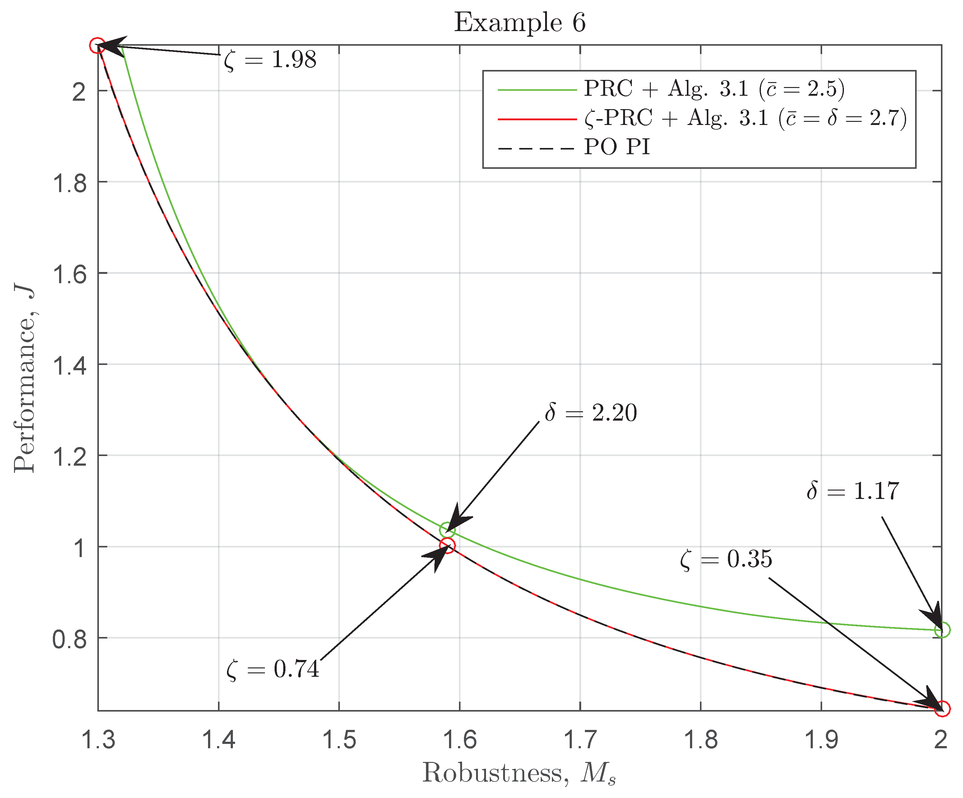
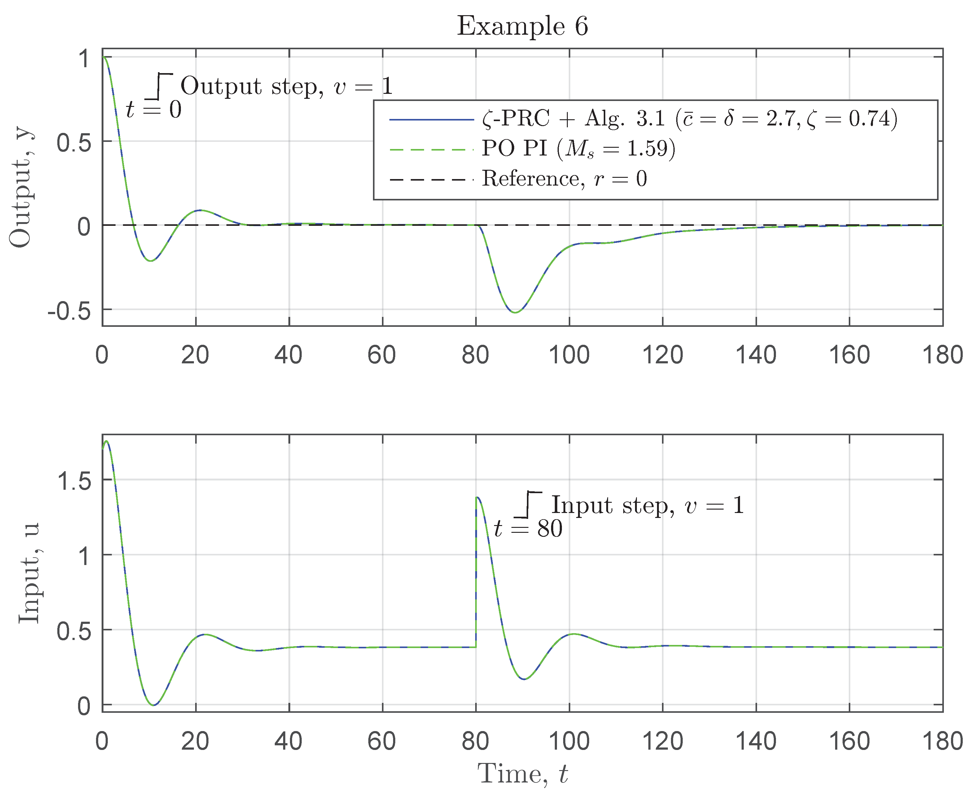
Example 6

ζ-PRC variant).

Consider the same process model as studied in Example 5. The model is approximated by an IPTD model, where the gain velocity is varied, $k=R_1\zeta =-0.145\zeta$, and time delay, $\tau =L=1.729$. In this example, we set the RTDE $\delta =\overline{c}=2.7$.

It can be seen in Figure 12 that the PO PI curve and the ζ-PRC curve are indistinguishable. This is quite a surprising result. In terms of the main performance objective $V_M$, we show in Table 13 that ζ-PRC is $\frac{V_{\zeta -PRC}}{V_{PRC}}=4e+3$ times better than $PRC$ variant.

Figure 12. Example 6. PI control of the higher order underdamped process model (Equation (48)). The figure illustrates the trade-off curves with the Pareto performance objective J (Equation (41)) and robustness $M_s$ (Equation (10)). It shows the PO PI controllers with robustness $M_s$ and the ζ-PRC + Algorithm 1 variant where the RTDE $\delta =\overline{c}=2.7$ is fixed and the main tuning parameter is ζ.

Table 13. Example 6. Comparing the following variants, ζ-PRC + Algorithm 1 with MP parameter and MTDE settings $\overline{c}=\delta =2.7$ and $\zeta =0.74$, and the PRC + Algorithm 1 with MP parameter setting $\overline{c}=2.5$, using the main performance $V_M$ defined in Equation (42).

Variant	PRC	$\mathit{\zeta }$-PRC
$V_M$/e-4	83.6	0.02

The time-domain responses, for a prescribed robustness $M_s=1.59$, are illustrated in Figure 13. As a consequence of the above, these responses are also indistinguishable. The corresponding PI controller parameters, indices and margins are given in Table 14.

Figure 13. Example 6. PI control of the higher order underdamped process model (Equation (48)). The figure illustrates the time-domain responses, given a prescribed robustness $M_s=1.59$, for the following methods: the PO PI and the ζ-PRC + Algorithm 1 variant with MP parameter and MTDE settings $\overline{c}=\delta =2.7$, and tuning parameter $\zeta =0.74$. An output disturbance unit step is presented at time $t=0$ and an input disturbance unit step at time $t=80$.

Table 14. Example 6. The corresponding controller parameter, indices and margins are given for prescribed robustness $M_s=1.59$. ζ-PRC + Algorithm 1.

	$\mathit{\zeta }$-Alg. 1	PO PI
$K_p$	−1.70	−1.70
$T_i$	14.82	14.90
${\mathrm{IAE}}_{vy}$	5.88	5.88
${\mathrm{IAE}}_{vu}$	8.69	8.72
J	1.00	1.00
TV	5.06	5.06
GM	11.85	11.84
PM	44.15	44.20
DM	2.74	2.74
$M_s$	1.59	1.59

6. Discussion

Remarks to Section 3

It can be shown that the PM can be given as follows

$$\begin{array}{c}\hfill PM=\delta \sqrt{f}\alpha ,\end{array}$$

(49)

for the PM in radians (see also [1,2]).

7. Concluding Remarks

The discussion and concluding remarks are itemised as follows.

• The method in [1,2] is further developed with more optimal MP tuning parameters as well as tuning for some special case integrating systems.
• Two optimal settings for the MP parameter are presented in Section 4. These are optimal in the sense that they minimise the main performance objective $V_M$ on two different aspects. Interestingly, one of the MP parameters may (arguably) be deduced from approximating the time delay with a (2, 1) Pade approximation in Section 3.3.
• In the case of a small or zero time delay $\tau =0$, we propose a variant in which the MTDE $d{\tau }_{max}$ is the tuning parameter.
• Note that for an IPTD model, the SIMC tuned PI controllers are seen far from optimal, i.e., PO (or (almost) equivalently, Algorithm 1 with the MP parameter setting as $\overline{c}=2.5$). See Section 4.
• The presented method (and variants of this) is successfully demonstrated and compared to the SIMC and PO PI controllers on numerous motivated process model examples in Section 5.
• Note that, for the higher order process models in Examples 4 and 5, we use the PRC model reduction technique, which is generally easier to apply than the half-rule technique proposed in [12]. The half-rule technique is not compatible with handling complex poles.
• Some surprisingly optimal results are documented for Example 6, where a tuning method based on varying the gain velocity, $k=\zeta R_1$, ($R_1$, is the ZN unit reaction rate), i.e., the tuning parameter is $\zeta$. Note that setting the RTDE $\delta =\overline{c}$ (i.e., an ad hoc choice) equal a constant is advisable.
• Note that the results in Section 5 are based on the original (possible) higher order models. The approximated IPTD models are only used for the PI controller design.