Article

A New Oren–Nayar Shape-from-Shading Approach for 3D Reconstruction Using High-Order Godunov-Based Scheme

1
School of Optoelectronic Engineering, Xi’an Technological University, Xi’an 710021, China
2
Shaanxi Province Key Laboratory of Optoelectronic Measurement and Instrument Technology, Xi’an Technological University, Xi’an 710021, China
*
Author to whom correspondence should be addressed.
Algorithms 2018, 11(5), 75; https://doi.org/10.3390/a11050075
Submission received: 17 April 2018 / Revised: 13 May 2018 / Accepted: 16 May 2018 / Published: 18 May 2018

Abstract

:
3D shape reconstruction from images has been an important topic in the field of robot vision. Shape-From-Shading (SFS) is a classical method for determining the shape of a 3D surface from a one intensity image. The Lambertian reflectance is a fundamental assumption in conventional SFS approaches. Unfortunately, when applied to characterize the reflection attribute of the diffuse reflection, the Lambertian model is tested to be inexact. In this paper, we present a new SFS approach for 3D reconstruction of diffuse surfaces whose reflection attribute is approximated by the Oren–Nayar reflection model. The partial differential Image Irradiance Equation (IIR) is set up with this model under a single distant point light source and an orthographic camera projection whose direction coincides with the light source. Then, the IIR is converted into an eikonal equation by solving a quadratic equation that includes the 3D surface shape. The viscosity solution of the resulting eikonal equation is approximated by using the high-order Godunov-based scheme that is accelerated by means of an alternating sweeping strategy. We conduct the experiments on synthetic and real-world images, and the experimental results illustrate the effectiveness of the presented approach.

1. Introduction

3D shape reconstruction from images has been an important topic in the field of robot vision. Shape-From-shading (SFS), initiated by Horn [1,2], is a classical method for determining the shape of a 3D surface from a one intensity image. He described the SFS problem by the so-called Image Irradiance Equation (IIR), which is a nonlinear Partial Differential Equation (PDE) of the first-order, and demonstrates the relationship between the 3D surface shape and its relevant 2D image intensity variations.
There are primarily two steps when processing an SFS problem. The first step is that of setting up a partial differential IIR under certain assumptions. The assumptions are used to model the image formation process and are dependent on the reflection attribute of the surface, the light source, and the camera. The second step is that of building a numerical scheme to acquire a solution of the IIR, which is the 3D shape of the known intensity image. Since the pioneering work of Horn, the majority of the SFS works focuses on how to build a numerical scheme with the simple Lambertian model; thus, many SFS algorithms have been reported (one can see the extensive list of the references in the three surveys [3,4,5]). According to Zhang et al. [4], Durou et al. [5], and Tozza and Falcone [6], these algorithms are roughly divided into two categories: PDE-based approaches and optimization approaches. The early work of Horn [1] based on the method of characteristics and the viscosity solution theories-based methods [7,8,9,10,11] all belong to the first category. It is worth mentioning that Rouy and Tourin [7] first formulated the SFS problem as a Hamilton–Jacobi–Bellman (HJB) PDE, whose solution is obtained through the viscosity solution theories. Kimmel and Sethian [8] converted the partial differential IIR with Lambertian reflection model into an eikonal PDE. They adopted the fast-marching method [12] to compute its viscosity solution. These approaches [1,7,8] are based on an orthographic camera projection. For a perspective camera projection, Prados and Faugeras [9] associated the partial differential IIR with a Hamiltonian and approximated its viscosity solution using optimal control strategy on the basis of the work [7]. Breuß et al. [10,11] studied analytically and numerically the perspective SFS model introduced by Prados and Faugeras [9] and the related Hamilton–Jacobi (HJ) PDE. Also, they proved the convergence of a finite-difference scheme and a semi-Lagrangian scheme for the HJ PDE. The second category includes the minimization methods for the variational problem. Lee and Kuo [13] presented an iterative SFS method under the perspective camera projection. They approximated a smooth surface by the union of triangular surface patches which involved only the height variables. The shape was recovered by linearizing the reflectance map and minimizing a quadratic cost functional. Courteille et al. [14] introduced some form of regularization, by formulating a PDE-based weak perspective or perspective IIR in terms of a spline basis. We want to mention the work by Quéau et al. [15], who combined the advantages of PDE-based approaches and optimization approaches, and created a generic variational solution based on PDEs that is suitable for SFS under natural illumination and can handle a variety of scenarios for the camera and the lighting. Finally, in addition to these work, we should also mention that a latest work by Scheffler et al. [16], who gave a novel graph theoretical framework built on cycle bases. They proposed a linear program for realizing the approach to solve the disambiguation problem for SFS.
As for the modeling process of the surface reflection, few are reported in the SFS literature. Generally, the Lambertian reflectance is a fundamental assumption in conventional SFS approaches for approximating the reflection attribute of the diffuse reflection. Unfortunately, the Lambertian model has been tested to be inexact, especially for rough diffuse surfaces [17]. Samaras and Metaxas [18] adopted the Deformable Models and Oren–Nayar [17] model to construct an approach for non-Lambertian SFS and estimating the light direction. Ragheb and Hancock [19] also reported a non-Lambertian SFS with the Oren–Nayar model and presented two solutions: the analytic solution and the lookup table. Ahmed and Farag [20] gave several non-Lambertian SFS models and solved the partial differential IIR using the Lax-Friedrichs sweeping scheme [21]. Tozza and Falcone [6] proposed a unified formulation for several non-Lambertian SFS models, solved by a semi-Lagrangian approximation scheme and proved a convergence result. In these non-Lambertian SFS approaches, the distant point light source and the orthographic camera projection are adopted. Because of their simplicity, our current study is based on these models. Of course, recent research focuses on the more realistic imaging model, including a nearby point light source and perspective camera projection. Ahmed and Farag [22] used the model proposed by Prados and Faugeras [9], where the point light source is ideally attached to the camera’s projection center, and a light attenuation term 1/r2 (r defines the distance between the position of the light source and the 3D surface point) has been considered in order to eliminate the ambiguity regarding convex and concave that makes the non-Lambertian SFS problem ill-posed. Moreover, Ju et al. [23] extended the work of Galliani et al. [24]: they used spherical surface parameterization to Oren–Nayar reflection model and thus could resolve an arbitrary position of the point light source. Nevertheless, the solving process needs transform the fast-marching method described in Cartesian coordinates [12] into spherical coordinates.
In this paper, we present a new Oren–Nayar SFS approach for 3D reconstruction of diffuse surfaces by extending our work [25]. The Oren–Nayar reflection model is also applied to approximate the reflection attribute of the diffuse reflection. Then, a partial differential IIR with this model is set up under a single distant point light source and an orthographic camera projection whose direction coincides with the light source. Although several works [6,20,26] have been reported in this situation, our main contribution is that we convert the IIR into a standard eikonal PDE by solving a quadratic equation which includes the 3D surface shape, after which we try to obtain the viscosity solution of the resulting eikonal equation by using the high-order Godunov-based scheme.

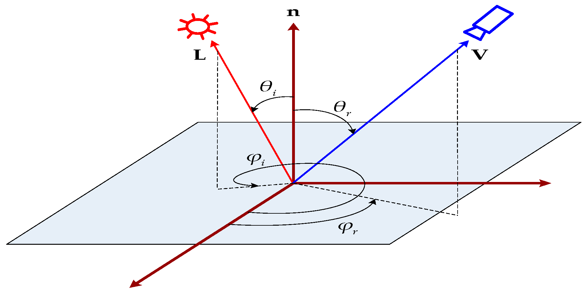
2. IIR for Oren–Nayar Reflectance

Under the basis that the image plane of the camera is an x - y plane and the camera’s optical axis is a z -axis, the SFS problem is able to be expressed as reconstructing a 3D surface, z ( x , y ) , which satisfies the partial differential IIR [1]:
I ( x , y ) = R ( z x , z y ) = R ( p ( x , y ) , q ( x , y ) ) ,
where I ( x , y ) is the image irradiance that is considered to be equal to the image intensity, p ( x , y ) and q ( x , y ) respectively stand for the first partial derivatives of the surface z ( x , y ) with respect to x and y , and R is the reflectance map derived from the reflection model.
Assuming that the camera performs an orthographic projection of a surface which is irradiated by a single point light source placed distantly from the surface, we can adopt the formulation as follows to describe the normal vector n at a 3D surface point ( x , y , z ( x , y ) ) ,
n = [ p , q , 1 ] .
The reflected radiance of an ideal diffuse surface obeys Lambert’s law, which can be expressed by
L r ( θ i ) = ρ π I 0 cos θ i ,
where θ i , as illustrated in Figure 1, is the angle between the normal vector n , and the incident direction of the point light source L , ρ is the albedo of diffuse surfaces that is constant in this paper, and I 0 is the radiant intensity of the light source. However, for a typical real diffuse surface, the Lambertian reflection model is tested to be an inexact approximation of the diffuse component of the surface reflection [17,25]. To eliminate the inexactness for diffuse reflection deriving from the assumption of the Lambertian model, Oren and Nayar [17] produced an advanced reflection model for rough diffuse surfaces where the roughness model has been used. The roughness model considers that the surface is constituted by extended symmetric V-shaped cavities, where every V-cavity consists of two planar facets which are considered to obey the Lambert’s law. The roughness of the surface is determined by a probability function of the planar facet orientations. Moreover, using a Gaussian distribution, with the reflection geometry shown in Figure 1, a formulation for the surface reflected radiance L r is addressed:
L r ( ϕ i , θ i ; ϕ r , θ r ; σ ) = ρ π I 0 cos θ i ( A ( σ ) + B ( σ ) sin α tan β max [ cos ( ϕ r ϕ i ) , 0 ] ) ,
where α = max [ θ i , θ r ] , β = min [ θ i , θ r ] , A ( σ ) = 1 0.5 σ 2 / ( σ 2 + 0.33 ) and B ( σ ) = 0.45 σ 2 / ( σ 2 + 0.09 ) . The parameter σ is standed as a measure of the surface roughness, and it represents the standard deviation of the Gaussian distribution.
Considering that the direction of the point light source L coincides with the camera’s direction V , we have ϕ i = ϕ r , θ i = θ r , and α = β . Consequently, Equation (4) can be simplified to
L r ( θ i ; σ ) = ρ π I 0 ( A ( σ ) cos θ i + B ( σ ) sin 2 θ i ) .
Generally speaking, Equation (5) can only be established under the assumptions that are a single distant point light source and an orthographic camera projection whose direction coincides with the light source or a nearby point light source attached to the projection center of the camera performing a perspective projection. If the camera’s direction does not coincide with the light source, our approach is no longer suitable, in which case one can refer to the work of [6,23]. Defining that the unit vectors of L and V are all [ 0 , 0 , 1 ] and since θ i is the angle between the normal vector n and L , we have
cos θ i = L L n n = 1 p 2 + q 2 + 1 = 1 z ( x , y ) 2 + 1 , sin 2 θ i = 1 cos 2 θ i = z ( x , y ) 2 z ( x , y ) 2 + 1 .
According to [1], taking Equation (6) into Equation (5), the reflectance map derived from the Oren–Nayar model is formulated as follows and now we can express the partial differential IIR for the Oren–Nayar reflectance:
R ( p , q ) = A ( σ ) 1 z ( x , y ) 2 + 1 + B ( σ ) z ( x , y ) 2 z ( x , y ) 2 + 1 = I ( x , y ) .
A similar IIR for the Oren–Nayar SFS has been reported in [26] and can be solved by a semi-Lagrangian approximation scheme. Here we convert the IIR into a standard eikonal PDE which will be solved by the high-order Godunov-based scheme. Obviously, the formulation (7) is able to be characterized by a quadratic equation in the variable z ( x , y ) 2 + 1 . Applying the change of variable g = z ( x , y ) 2 + 1 , Equation (7) is formulated as
( I ( x , y ) B ( σ ) ) g 2 A ( σ ) g + B ( σ ) = 0 .
Calculating Equation (8) and satisfying g 1 , we have
g = 2 B ( σ ) A ( σ ) A ( σ ) 2 4 ( I ( x , y ) B ( σ ) ) B ( σ ) .
Thus, the SFS problem (7) has been reformulated as a standard eikonal PDE:
{ z ( x , y ) = g 2 1 x Ω , z ( x , y ) = ϕ ( x , y ) x Ω ,
where ϕ ( x , y ) is a boundary condition and Ω is a given image domain.

3. Numerical Algorithm for Solving the Resulting Eikonal PDE

In this section, we employ the high-order Godunov-based scheme [27] that is accelerated by alternating sweeping strategy [28,29] to solve the viscosity solution of the resulting eikonal PDE (10).

3.1. High-Order Godunov-Based Scheme

Consider a uniform discretization { ( x m , y n ) = ( m s , n s ) , m = 1 , 2 , , r , n = 1 , 2 , , c } of the given image domain Ω whose resolution and grid size are r × c and s × s , respectively. Now our goal is to get a discrete solution z m , n = z ( x m , y n ) of the unknown 3D surface z ( x , y ) .
A first-order Godunov-based scheme proposed in [7,29] is employed to discretize resulting eikonal PDE (10):
max [ z m , n z m 1 , n s , z m + 1 , n z m , n s , 0 ] 2 + max [ z m , n z m , n 1 s , z m , n + 1 z m , n s , 0 ] 2 = F m , n 2 ,
where F m , n = g m , n 2 1 . The substitution of z a = min [ z m 1 , n , z m + 1 , n ] , z b = min [ z m , n 1 , z m , n + 1 ] and
{ x } + = { x x 0 0 x < 0
into Equation (11), we have
[ { z m , n z a s } + ] 2 + [ { z m , n z b s } + ] 2 = F m , n 2 .
Hence, the first-order scheme viscosity solution of Equation (13) can be obtained thusly:
z m , n = { z a + z b + 2 s 2 F m , n 2 ( z a z b ) 2 2 | z a z b | < s F m , n , min [ z a , z b ] + s F m , n | z a z b | s F m , n .
To build a higher-order scheme, the p m , n and q m , n with higher-order accuracy need to be approximated. According to [27], since the third-order Weighted Essentially Non-Oscillatory (WENO) scheme has a uniform high order accuracy and is more efficient and robust than other schemes (e.g., the Essentially Non-Oscillatory (ENO) scheme), we also choose to employ the third-order WENO approximations.
{ max [ z m , n n e w z 1 s , 0 ] } 2 + { max [ z m , n n e w z 2 s , 0 ] } 2 = F m , n 2 ,
where
z 1 = min [ ( z m , n o l d s p m , n ) , ( z m , n o l d + s p m , n + ) ] , z 2 = min [ ( z m , n o l d s q m , n ) , ( z m , n o l d + s q m , n + ) ] ,
with
p m , n = ( 1 α ) ( z m + 1 , n z m 1 , n 2 s ) + α ( 3 z m , n 4 z m 1 , n + z m 2 , n 2 s ) , p m , n + = ( 1 α + ) ( z m + 1 , n z m 1 , n 2 s ) + α + ( z m + 2 , n + 4 z m + 1 , n 3 z m , n 2 s ) .
Here
α = 1 1 + 2 β 2 ,   β = μ + ( z m , n 2 z m 1 , n + z m 2 , n ) 2 μ + ( z m + 1 , n 2 z m , n + z m 1 , n ) 2 , α + = 1 1 + 2 β + 2 ,   β + = μ + ( z m + 2 , n 2 z m + 1 , n + z m , n ) 2 μ + ( z m + 1 , n 2 z m , n + z m 1 , n ) 2 ,
where μ is a very small number keeping the denominator from getting too close to 0. In a similar way, q m , n and q m , n + are specified.
Thus, the higher-order scheme viscosity solution of Equation (13) can be obtained:
z m , n n e w = { z 1 + z 2 + 2 s 2 F m , n 2 ( z 1 z 2 ) 2 2 | z 1 z 2 | < s F m , n , min [ z 1 , z 2 ] + s F m , n | z 1 z 2 | s F m , n .

3.2. Alternating Sweeping Strategy for Godunov-Based Scheme

To speed up the convergence of the high-order Godunov-based scheme, the philosophy of alternating sweeping strategy and Gauss–Seidel iterations [28,29] are used as follows. The newest available values for z are adopted when we calculate the derivatives p m , n , p m , n + , and q m , n , q m , n + . Simultaneously, the iterations of the scheme do not only sweep in a single direction, but in the four alternating directions as follows: (a) from upper left to lower right; (b) from lower left to upper right; (c) from lower right to upper left; (d) from upper right to lower left. As can be clearly demonstrated that varied values z m ± 2 , n , z m ± 1 , n and z m , n ± 2 , z m , n ± 1 will be taken into account according to the current sweeping direction within the preceding cycle.
The high-order Godunov-based scheme accelerated by an alternating sweeping strategy is summarized in the following way:
(1)
Initialization: On the boundary Ω we set the grid points to be accurate values, i.e., z m , n 0 = ϕ m , n , which are unchanged during the iterations of the scheme. The approximated solution from the first-order Godunov-based scheme is applied as the initial guess for all other grid points.
(2)
Iterations with Alternating Sweepings Orderings: We calculate z m , n n e w at ( i + 1 ) th iteration, updated by the rules (19) using Gauss–Seidel iterations with the following four alternating sweepings orderings:
m = 1 : r ,   n = 1 : c ;
m = r : 1 ,   n = 1 : c ;
m = r : 1 ,   n = c : 1 ;
m = 1 : r , n = c : 1 .
(3)
Convergence Test: If z i + 1 z i L 1 δ , where δ > 0 is a known threshold value, the scheme stops and converges, or else comes back to (2). In this paper, δ = 10 5 is taken.

4. Experimental Results

The effectiveness of the presented approach is assessed using several experiments on synthetic and real-world images. All the experiments were conducted on a general-purpose personal computer with an Intel Core i5-3570 CPU and 4 GB of DDR3 memory. We implemented all the approaches in Matlab, using C mex functions under Microsoft Windows operating system environments.

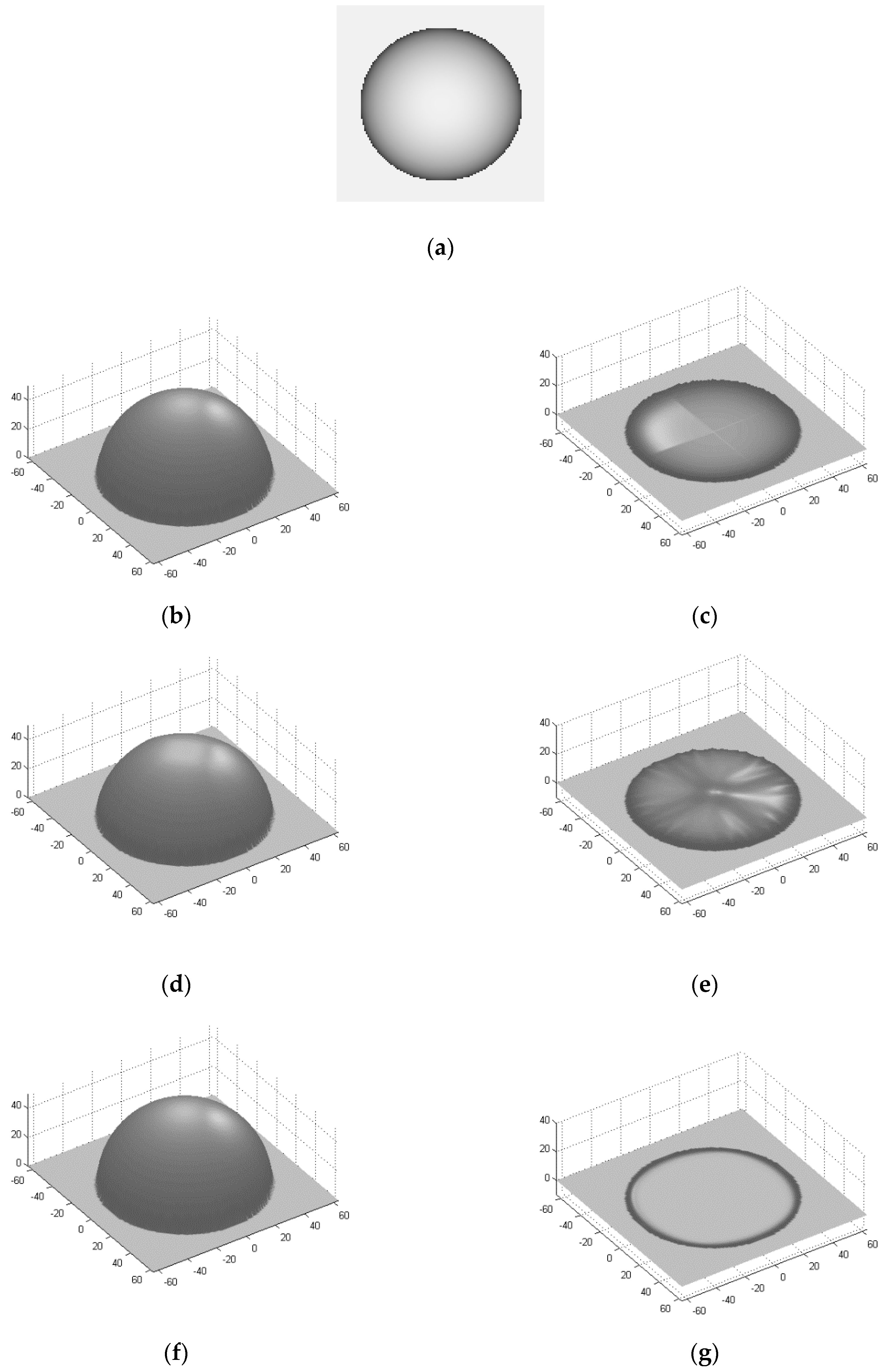
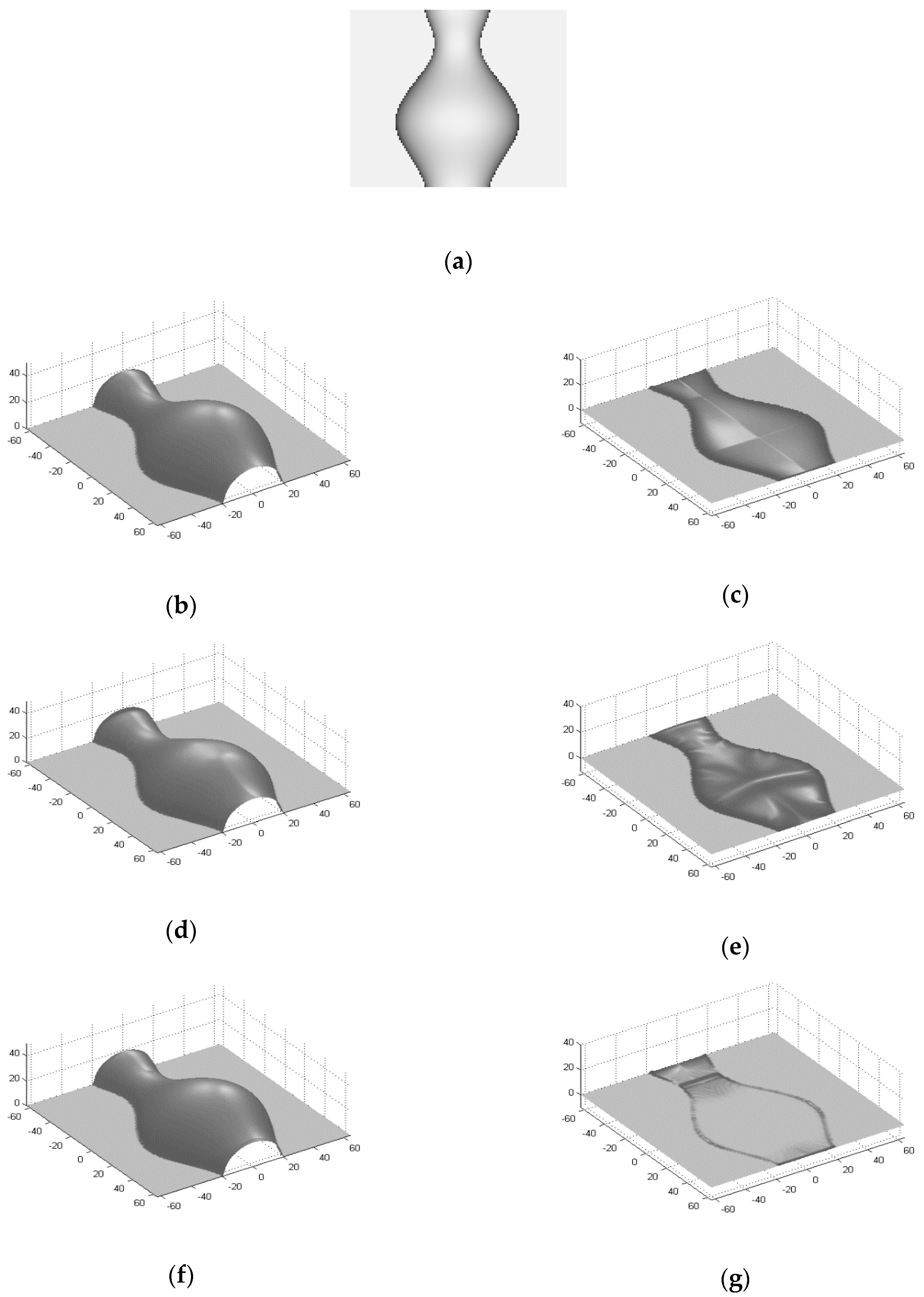
4.1. Experimental Results on Synthetic Images

A synthetic image of the sphere which was produced using the following formulation (20) was employed in our experiments:
z ( x , y ) = R 2 x 2 y 2 ,
where ( x , y ) [ 63 , 64 ] × [ 63 , 64 ] and R = 50 is the sphere’s radius. Another synthetic image of the vase which was produced using the following formulation (21) was also employed:
z ( x , y ) = f ( y ) 2 x 2 ,
where f ( y ) = 0.025 ( 6 y 1 ) ( 2 y + 1 ) ( 2 y 1 ) 2 ( 3 y + 2 ) 2 + 0.15 and ( x , y ) [ 0.5 , 0.5 ] × [ 0.5 , 0.5 ] . We can map the x and y values to [ 63 , 64 ] and scale z ( x , y ) by a factor of 128. This yields a maximum height value of approximately 36.55. Their original height maps are demonstrated in Figure 2.
The two images are generated by the model in this paper with the direction vectors of the point light source and the camera all being [ 0 , 0 , 1 ] T . The variant approach of Kimmel and Sethian [8] and the approach of Ahmed and Farag [20] are used to compare with our presented approach. It has been noted that the approach of Ahmed and Farag [20] applied the Lax–Friedrichs sweeping scheme to solve the Oren–Nayar SFS, and that the existing approach of Kimmel and Sethian [8] used the first-order Godunov-based scheme to solve the Lambertian SFS and therefore cannot directly solve the Oren–Nayar SFS. However, it is able to solve our partial differential IIR (10) directly. We define the first-order Godunov-based scheme that is accelerated by an alternating sweeping strategy for the Oren–Nayar SFS as the variant approach of Kimmel and Sethian [8].
The experimental results of the sphere are illustrated in Figure 3. Figure 3a shows the synthetic intensity image which is adopted for the 3D reconstruction with the parameter set: σ = 0.2 . Figure 3b demonstrates the reconstructed height map using the variant approach of Kimmel and Sethian [8] and the known Dirichlet boundary condition z = ϕ on Ω , while the error map with the original height map is shown in Figure 3c. Figure 3d demonstrates the reconstructed height map using the approach of Ahmed and Farag [20], while the error map with the original height map is shown in Figure 3e. Figure 3f demonstrates the reconstructed height map using our presented approach with the known Dirichlet boundary condition z = ϕ on Ω , while the error map with the original height map is shown in Figure 3g. Finally, Figure 4 illustrates the corresponding experimental results of the synthetic vase.
Figure 3 and Figure 4 show that the variant approach of Kimmel and Sethian [8], the approach of Ahmed and Farag [20], and our presented approach can all obtain satisfactory reconstructed results of the diffuse surfaces. Moreover, we can further see that our presented approach gets a higher accuracy and smaller errors than the variant approach of Kimmel and Sethian [8] and the approach of Ahmed and Farag [20].
To further demonstrate the effectiveness of our presented approach, a quantitative comparison between the variant approach of Kimmel and Sethian [8], the approach of Ahmed and Farag [20], and our presented approach is adopted by using the CPU time, the Mean Absolute Error (MAE), and the Root Mean Square Error (RMSE). Table 1 lists the comparisons of the three approaches for the synthetic sphere and vase images. As is directly seen, our presented approach shows better performance in the reconstructed errors than the variant approach of Kimmel and Sethian [8], as well as than the approach of Ahmed and Farag [20] in all the images which we performed. The MAE and RMSE of our proposed approach are about one-fiftieth and one-twentieth of the variant approach of Kimmel and Sethian [8] for the sphere, and about one-seventh and one-fourth for the vase, respectively. The approach of Ahmed and Farag [20] shows a slightly worse performance; maybe it is difficult to find a good estimate for the artificial viscosity term. However, our presented approach requires longer CPU time than the variant approach of Kimmel and Sethian [8], because the former adopts a complex high-order approximation scheme.

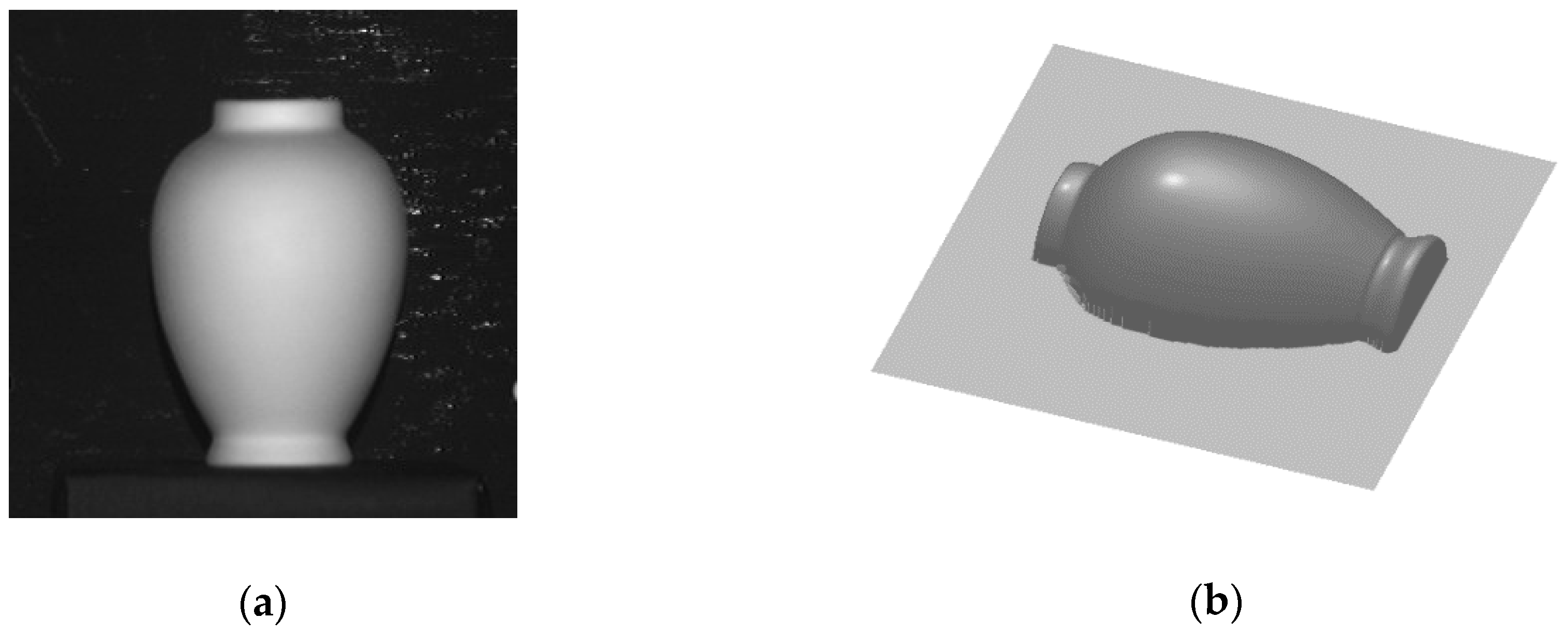
4.2. Experimental Results on Real-World Image

In order to evaluate the performance of our presented approach for real diffuse surfaces, we performed it on a real-world image and compared the reconstructed result with the existing approach of Kimmel and Sethian [8], the variant approach of Kimmel and Sethian [8], and the approach of Ahmed and Farag [20]. The image is the real-world vase used in the surveys [4,5], which is shown in Figure 5a. Figure 5b gives the ground truth referred to [5]. Figure 5c–f illustrate the reconstructed height maps using the approach of Kimmel and Sethian [8] with exact height values at each singular point, the variant approach of Kimmel and Sethian [8] with the known Dirichlet boundary condition z = ϕ on Ω , the approach of Ahmed and Farag [20], and our presented approach with the known Dirichlet boundary condition z = ϕ on Ω , respectively.
Similarly, we calculated the MAE and RMSE errors of these approaches and the comparisons results are listed in Table 2. From the reconstructed results illustrated in Figure 5c–f, we can see that our presented approach and the variant approach of Kimmel and Sethian [8] are more vivid than the approach of Kimmel and Sethian [8]. The same conclusion can be drawn from Table 2: our presented approach shows best performance since our approach employs the advanced reflection model for diffuse surfaces and high-order accurate numerical scheme. Recall that the approach of Kimmel and Sethian [8] assumes the Lambertian reflection model for diffuse surfaces. As previously, the approach of Ahmed and Farag [20] shows a slightly worse performance as can be seen from Figure 5e.

5. Conclusions

This paper reports a new Oren–Nayar SFS approach for 3D reconstruction of diffuse surfaces. We employed a Oren–Nayar reflection model instead of Lambertian model to approximate the reflection attribute of the diffuse reflection. The partial differential IIR for Oren–Nayar reflectance was set up with the model that the direction of the distant point light source is the same as the camera performing an orthographic projection. A standard eikonal PDE was derived from the IIR by solving a quadratic equation in the variable which includes of the 3D surface shape, and we obtained the viscosity solution of the resulting eikonal PDE using the high-order Godunov-based scheme that was accelerated by the philosophy of alternating sweeping strategy and Gauss–Seidel iterations. Experiments were conducted on synthetic and real-word images and the experimental results illustrate that our presented approach is effective and can get a higher accuracy than the first-order Godunov-based scheme and the Lax-Friedrichs scheme.
Frankly speaking, the presented approach in the paper can be only used in the situation with a single distant point light source and an orthographic camera projection whose direction coincides with the light source. Nevertheless, we believe that the idea of solving the quadratic IIR can be employed to alternately solve the SFS problem with a nearby point light source attached to the projection center of the camera performing a perspective projection. At the same time, the light attenuation term can be considered in order to eliminate the ambiguity regarding convex and concave that makes the SFS problem ill-posed. This work will be explored in the future.

Author Contributions

Both authors contributed to the research work. G.W. presented the approach and carried out the experiments; Y.C. and G.W. analyzed and processed the data; G.W. wrote this manuscript.

Funding

This research was funded by [Natural Science Basic Research Plan in Shaanxi Province of China] grant number [2016JM6041], [Scientific Research Program Funded by Shaanxi Provincial Education Department] grant number [15JK1351] and [National Natural Science Foundation of China] grant number [61102144].

Acknowledgments

The work is partly supported by the Natural Science Basic Research Plan in Shaanxi Province of China (No. 2016JM6041), Scientific Research Program Funded by Shaanxi Provincial Education Department (No. 15JK1351) and National Natural Science Foundation of China (No. 61102144).

Conflicts of Interest

All the authors declare that they have no conflict of interest.

References

  1. Horn, B.K.P. Shape from Shading: A Method for Obtaining the Shape of a Smooth Opaque Object from One View. Ph.D. Thesis, Massachusetts Institute of Technology, Cambridge, MA, USA, 1970. [Google Scholar]
  2. Horn, B.K.P.; Brooks, M.J. The variational approach to shape from shading. Comput. Vis. Graph. Image Process. 1986, 33, 174–208. [Google Scholar] [CrossRef]
  3. Horn, B.K.P.; Brooks, M.J. Shape from Shading; MIT Press: Cambridge, MA, USA, 1989; ISBN 978-0-262-08183-2. [Google Scholar]
  4. Zhang, R.; Tsai, P.-S.; Cryer, J.E.; Shah, M. Shape from shading: A survey. IEEE Trans. Pattern Anal. Mach. Intell. 1999, 21, 690–706. [Google Scholar] [CrossRef]
  5. Durou, J.-D.; Falcone, M.; Sagona, M. Numerical methods for shape-from-shading: A new survey with benchmarks. Comput. Vis. Image Underst. 2008, 109, 22–43. [Google Scholar] [CrossRef]
  6. Tozza, S.; Falcone, M. Analysis and approximation of some shape-from-shading models for non-Lambertian surfaces. J. Math. Imaging Vis. 2016, 55, 153–178. [Google Scholar] [CrossRef]
  7. Rouy, E.; Tourin, A. A viscosity solutions approach to shape-from-shading. SIAM J. Numer. Anal. 1992, 29, 867–884. [Google Scholar] [CrossRef]
  8. Kimmel, R.; Sethian, J.A. Optimal algorithm for shape from shading and path planning. J. Math. Imaging Vis. 2001, 14, 237–244. [Google Scholar] [CrossRef]
  9. Prados, E.; Camilli, F.; Faugeras, O. A unifying and rigorous shape from shading method adapted to realistic data and applications. J. Math. Imaging Vis. 2006, 25, 307–328. [Google Scholar] [CrossRef] [Green Version]
  10. Breuß, M.; Cristiani, E.; Durou, J.-D.; Falcone, M.; Vogel, O. Numerical algorithms for perspective shape from shading. Kybernetika 2010, 46, 207–225. [Google Scholar]
  11. Breuß, M.; Cristiani, E.; Durou, J.-D.; Falcone, M.; Vogel, O. Perspective shape from shading: Ambiguity analysis and numerical approximations. SIAM J. Imaging Sci. 2012, 5, 311–342. [Google Scholar] [CrossRef]
  12. Sethian, J.A. Fast marching methods. SIAM Rev. 1999, 41, 199–235. [Google Scholar] [CrossRef]
  13. Lee, K.M.; Kuo, C.-C.J. Shape from shading with perspective projection. Comput. Vis. Graph. Image Process. 1994, 59, 202–212. [Google Scholar] [CrossRef]
  14. Courteille, F.; Crouzil, A.; Durou, J.-D.; Gurdjos, P. 3D-spline reconstruction using shape from shading: Spline from shading. Image Vis. Comput. 2008, 26, 466–479. [Google Scholar] [CrossRef]
  15. Quéau, Y.; Mélou, J.; Castan, F.; Cremers, D.; Durou, J.-D. A variational approach to shape-from-shading under natural illumination. In Proceedings of the International Workshop on Energy Minimization Methods in Computer Vision and Pattern Recognition (EMMCVPR 2017), Venice, Italy, 30 October–1 November 2017; Pelillo, M., Hancock, E., Eds.; Springer International Publishing AG: Cham, Switzerland, 2018. [Google Scholar] [CrossRef]
  16. Scheffler, R.; Yarahmadi, A.M.; Breuß, M.; Köhler, E. A graph theoretic approach for shape from shading. In Proceedings of the International Workshop on Energy Minimization Methods in Computer Vision and Pattern Recognition (EMMCVPR 2017), Venice, Italy, 30 October–1 November 2017; Pelillo, M., Hancock, E., Eds.; Springer International Publishing AG: Cham, Switzerland, 2018. [Google Scholar] [CrossRef]
  17. Oren, M.; Nayar, S.K. Generalization of the Lambertian model and implications for machine vision. Int. J. Comput. Vis. 1995, 14, 227–251. [Google Scholar] [CrossRef]
  18. Samaras, D.; Metaxas, D. Incorporating illumination constraints in deformable models for shape from shading and light direction estimation. IEEE Trans. Pattern Anal. Mach. Intell. 2003, 25, 247–260. [Google Scholar] [CrossRef]
  19. Ragheb, H.; Hancock, E.R. Surface radiance correction for shape from shading. Pattern Recognit. 2005, 38, 1574–1595. [Google Scholar] [CrossRef]
  20. Ahmed, A.H.; Farag, A.A. Shape from shading under various imaging conditions. In Proceedings of the IEEE Conference on Computer Vision and Pattern Recognition (CVPR 2007), Minneapolis, MN, USA, 17–22 June 2007; IEEE Press: Piscataway, NJ, USA, 2007. [Google Scholar] [CrossRef]
  21. Kao, C.-Y.; Osher, S.; Qian, J. Lax-Friedrichs sweeping scheme for static Hamilton-Jacobi equations. J. Comput. Phys. 2004, 196, 367–391. [Google Scholar] [CrossRef]
  22. Ahmed, A.H.; Farag, A.A. A new formulation for shape from shading for non-Lambertian surfaces. In Proceedings of the IEEE Conference on Computer Vision and Pattern Recognition (CVPR 2006), New York, NY, USA, 17–22 June 2006; IEEE Press: Piscataway, NJ, USA, 2006. [Google Scholar] [CrossRef]
  23. Ju, Y.C.; Tozza, S.; Breuß, M.; Bruhn, A.; Kleefeld, A. Generalised perspective shape from shading with Oren-Nayar reflectance. In Proceedings of the 24th British Machine Vision Conference (BMVC 2013), Bristol, UK, 9–13 September 2013; Burghardt, T., Damen, D., Mayol-Cuevas, W., Mirmehdi, M., Eds.; BMVA Press: Durham, UK, 2013. [Google Scholar] [CrossRef]
  24. Galliani, S.; Ju, Y.C.; Breuß, M.; Bruhn, A. Generalised perspective shape from shading in spherical coordinates. In Proceedings of the International Conference on Scale Space and Variational Methods in Computer Vision (SSVM 2013), Leibnitz, Austria, 2–6 June 2013; Kuijper, A., Bredies, K., Pock, T., Bischof, H., Eds.; Springer Press: Berlin/Heidelberg, Germany, 2013. [Google Scholar] [CrossRef]
  25. Wang, G.; Liu, S.; Han, J.; Zhang, X. A novel shape from shading algorithm for non-Lambertian surfaces. In Proceedings of the 3rd International Conference on Measuring Technology and Mechatronics Automation (ICMTMA 2011), Shangshai, China, 6–7 January 2011; IEEE Press: Piscataway, NJ, USA, 2011. [Google Scholar] [CrossRef]
  26. Tozza, S.; Falcone, M. A comparison of non-Lambertian models for the shape-from-shading problem. In New Perspectives in Shape Analysis; Breuß, M., Bruckstein, A., Maragos, P., Wuhrer, S., Eds.; Springer International Publishing AG: Cham, Switzerland, 2016; pp. 15–42. ISBN 978-3-319-24724-3. [Google Scholar] [CrossRef]
  27. Zhang, Y.-T.; Zhao, H.-K.; Qian, J. High order fast sweeping methods for static Hamilton-Jacobi equations. J. Sci. Comput. 2006, 29, 25–56. [Google Scholar] [CrossRef]
  28. Tsai, Y.-H.R.; Cheng, L.-T.; Osher, S.; Zhao, H.-K. Fast sweeping algorithms for a class of Hamilton-Jacobi equations. SIAM J. Numer. Anal. 2003, 41, 673–694. [Google Scholar] [CrossRef]
  29. Zhao, H.-K. A fast sweeping method for eikonal equations. Math. Comput. 2005, 74, 603–627. [Google Scholar] [CrossRef]
Figure 1. Reflection geometry model of a 3D surface with the normal vector n . L and V are the incident direction of the point light source and the camera’s direction, respectively. ϕ i , ϕ r and θ i , θ r are their corresponding tilt and slant angles, respectively.
Algorithms 11 00075 g001
Figure 2. The original height maps: (a) the sphere; (b) the vase.
Algorithms 11 00075 g002
Figure 3. Experimental results of the synthetic sphere: (a) intensity image generated by Figure 2a with the parameter set: σ = 0.2 . (b) reconstructed height map using the variant approach of [8]; (c) error map of (b) with Figure 2a; (d) reconstructed height map using the approach of [20]; (e) error map of (d) with Figure 2a; (f) reconstructed height map using our presented approach; (g) error map of (f) with Figure 2a.
Algorithms 11 00075 g003
Figure 4. Experimental results of the synthetic vase: (a) intensity images generated by Figure 2b with the parameter set: σ = 0.2 . (b) reconstructed height map using the variant approach of [8]; (c) error map of (b) with Figure 2b; (d) reconstructed height map using the approach of [20]; (e) error map of (d) with Figure 2b; (f) reconstructed height map using our presented approach; (g) error map of (f) with Figure 2b.
Algorithms 11 00075 g004
Figure 5. Experimental results of the real-world vase: (a) real intensity image; (b) ground truth referred to [5]; (c) reconstructed height map using the approach of [8]; (d) reconstructed height map using the variant approach of [8]; (e) reconstructed height map using the approach of [20]; (f) reconstructed height map using our presented approach.
Algorithms 11 00075 g005aAlgorithms 11 00075 g005b
Table 1. Comparisons of approaches for the synthetic images.
ApproachesSphereVase
MAERMSECPU timeMAERMSECPU time
Variant approach of [8]0.69030.83800.006 s0.54640.65150.005 s
Approach of [20]1.06371.48870.276 s0.68521.08670.217 s
Presented approach0.01340.04150.093 s0.07930.15370.067 s
Table 2. Comparisons of approaches for the real-world vase.
ApproachesMAERMSE
Approach of [8]0.27310.3804
Variant approach of [8]0.18820.2429
Approach of [20]0.26480.3496
Presented approach0.07710.0987

