Abstract
In order to improve the dynamic quality of traditional sliding mode control for an active suspension system, an optimal sliding mode control (OSMC) based on a genetic algorithm (GA) is proposed. First, the overall structure and control principle of the active suspension system are introduced. Second, the mathematical model of the quarter car active suspension system is established. Third, a sliding mode control (SMC) controller is designed to manipulate the active force to control the active suspension system. Fourth, GA is applied to optimize the weight coefficients of an SMC switching function and the parameters of the control law. Finally, the simulation model is built based on MATLAB/Simulink (version 2014a), and the simulations are performed and analyzed with the proposed control strategy to identify its performance. The simulation results show that the OSMC controller tuned using a GA has better control performance than the traditional SMC controller.
1. Introduction
The suspension system is one of the most important parts of the vehicles, which can reduce the impact loads from the road to improve the automotive ride comfort and stability. Compared with the passive and semi-active suspension systems, the active suspension system can supply energy from an external source and generate force to achieve the desired performance [1]. The active suspension system is widely used in vehicles because of its outstanding control characteristic and performance.
The performance indicators for the vehicle suspension mainly consist of the ride comfort, suspension deflection, and road holding; however, these three indexes usually conflict with each other. For instance, improving the ride comfort leads to the increase of the suspension deflection and the decrease of the tire road holding [2]. As a result, it is essential to find an appropriate control strategy for the active suspension system to balance the relationships among the above three performance indexes effectively. Younes [3] proposed the minimum time controller design using singular perturbation method for a quarter car active suspension system. Peng Wang [4] proposed a new design method of fractional skyhook damping control for full-car suspension based on the principle of modal coordinate transformation. Huang [5] presented a novel control strategy for a nonlinear uncertain vehicle active suspension system without using any function approximators. Bououden [6] designed a robust predictive control for a nonlinear active suspension system. Kumar [7] introduced the self-tuned robust fractional order fuzzy PD (proportion and differential) controller for uncertain and nonlinear active suspension system, but their tuning method requires human experience to construct the fuzzy rules [8]. Bharali [9] proposed the linear quadratic regulator (LQR) and fuzzy logic controller for active suspension system, however, the SMC can remove the chattering which had been the main defect of the LQR control [10].
SMC is gradually applied in control fields, which has the advantages of good robustness to external disturbance and fast dynamic response, etc. Ayadi [11] applied the adaptive sliding mode controller on the experimental validation for electro-pneumatic system. Guermouche [12] presented the adaptive super twisting extended state observer-based sliding mode control for diesel engine air path subject to matched and unmatched disturbance. Benamor [13] put forward the robust adaptive sliding mode control for uncertain systems with unknown time-varying delay input. Devika [14] designed a sliding mode controller for MIMO (multi-input-multi-out) nonlinear systems so as to improve control performance. Ozer [15] presented the high order sliding mode control for active suspensions, which attenuates chattering effectively while preserving its robustness. However, it adds complexity to the calculations [16].
The switching function and control law are the critical parts of the sliding mode control according to the principles of variable-structure control [17]. Actually, these two parts determine the extent of chattering and the control effect of the SMC controller. Some scholars have applied the SMC on the control of various systems. Tuan [18] presented the adaptive neural network sliding mode control of shipboard container cranes considering actuator backlash. Alves [19] proposed a sliding mode controller for active suspension system with data acquisition delay. Yuvapriya [20] used the fractional order sliding mode controller to solve the vibration problem of full car active suspension system. Repecho [21] designed a robust sliding mode controller of a DC/DC boost converter (DC—direct current) with switching frequency regulation. However, most of the scholars only provided the range of values for parameters of the switching function and control law, and the final values of which are given straight away without any explanations and selection methods. Compared with the traditional sliding mode control, the OSMC optimizes the adjustable parameters of the switching function and control law by means of a genetic algorithm (GA).
GA [22,23] is closely related to industrial applications, which consider the optimization of parameters with constraints, targets, and dynamic components [24]. Nabavi [25] proposed a GA-based design and optimization method for micro-electromechanical systems unimorph piezoelectric energy harvesters that demonstrated an enhancement of energy harvesting efficiency by 31% in comparison with un-optimized harvesters. Gad et al. [26] optimized the fractional order PID (proportion, integral and differential) controller based on multi-objective GA. Almeida, Jr. [27] presented a GA for the optimization of the stacking sequence to improve the strength of a cylindrical shell under internal pressure.
In order to improve the control effect, this paper designs an OSMC controller tuned using a GA to control the active suspension system of the vehicle. The rest of this paper is organized as follows: Section 2 overviews the structure and control principle of the active suspension system, Section 3 studies the active suspension system modelling, Section 4 focuses on the SMC controller design, Section 5 describes the simulations, and the final section give the conclusions.
2. The Structure and Control Principle of the Active Suspension System
In addition to transferring the reaction force directly to the chassis, the design of the suspension system aims to relax the road surface impact, attenuate vibration, ensure vehicle ride comfort and stability control capacities. The active suspension system includes an actuator, a matching sensor, and a control unit that can input force and displacement to the suspension system based on the passive suspension system. The actuator can generate force according to the real-time changes of the road input and the vehicle status, thereby compensating for the disturbances produced by road irregularities and obtaining a good shock absorption effect [20]. The control principle of the active suspension system is shown in Figure 1.
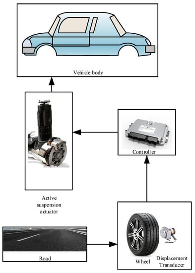
Figure 1.
Structure and control principle of the active suspension system.
As shown in Figure 1, the active suspension system consists of three parts: the wheel module, the controller module, and the actuator module. First, the controller receives the signals of the road information from the displacement sensor, and then the controller controls the output displacement of the actuators independently, thus controlling the posture of the vehicle. The displacement sensors installed on the wheels are used to transmit the vertical displacement caused by road irregularities to the controller.
3. Modeling of the Active Suspension System
3.1. Dynamic Model of Quarter Car Active Suspension System
As shown in Figure 1, the quarter car model is selected as the model of the suspension system, which is simple and can capture important characteristics of full model [3,28]. A quarter car active suspension model considered in this work is taken from Reference [29], as shown in Figure 2. From Figure 2 and Newton’s second law, the dynamic equations of the quarter car model are presented in Equation (1):
where and stand for the sprung mass and the unsprung mass, respectively, represents the spring stiffness between tire and road, denotes the spring stiffness between tire and car body, denotes the damping coefficient between tire and car body, indicates the control force output from actuator, is the vertical displacement of unsprung mass, denotes the vertical displacement of sprung mass, and represents the vertical displacement caused by road surface irregularity.
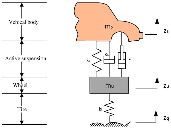
Figure 2.
Mechanical model of a quarter car active suspension system.
The state vector of the quarter car suspension system is selected as :
The state equation of the quarter car suspension system is established in Equation (3):
where is the output equation of the suspension system, the matrix , and are constants and with appropriate dimensions, the matrix is the disturbance vector input from the road, and the matrix is the control vector input from the controller. The matrices and are shown as follows:
3.2. Random Road Inputs Model
For the active suspension system, the vibration generated inside a vehicle body is usually ignored, and the unevenness of the road surface is the most important factor that affects the vehicle ride comfort. The model of random road surface is generally selected as the most commonly used in simulation, such that more results and greater significance can be obtained [30]. The expression for is shown in Equation (5):
where represents the lower frequency cut-offs, denotes the coefficient of the road irregularities, is the speed of the vehicle, is the reference space frequency, and is the white noise signal of the road.
According to the classification standard of the road roughness [31], the value of is and of the C level road is any value between 0.000128 and 0.000512. In this paper, the level C road is taken as the simulation road because of its large coverage in China. The random road’s simulation model based on MATLAB/Simulink (version 2014a, United States) is shown in Figure 3, and its data is displayed in Table 1. As a result, the input displacement of the level C road of the quarter car suspension with a speed of 20 m/s is shown in Figure 4.
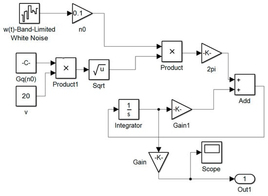
Figure 3.
Simulation model of a random road.

Table 1.
The simulation parameters of the random road.
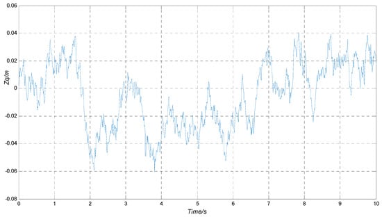
Figure 4.
The input displacement of the level C road in this paper.
3.3. Evaluation Index of the Suspension System
The optimization control of the suspension system is mainly used to raise the driving amenity, which is the main measure of the objective function. Typically, the evaluation of the suspension performance is subject to the monitoring of the passengers’ maximum absolute vertical acceleration (which relates to the ride comfort), wheel hop (which relates to the vehicle stability on the road and displacement, and (which relates to the suspension rattle space) in the suspension system [32]. In order to trade off the three performance requirements, a quadratic objective function expression is taken as the performance index based on the quadratic optimal control theory, which is shown in Equation (6):
where represents the total travel time of the vehicle, and denote the weight coefficients of the wheel hop and the displacement in the suspension system, respectively.
4. The OSMC Controller Design
As a variable structure control strategy, the SMC strategy is different from other control strategies because of its discontinuity, which ensures the structure of the system can change over time. The variable structure control with sliding mode aims to lead the state trajectory of the system to a surface in the state space and ensure that it holds to this surface by means of a high-speed switching control law [19]. The whole design process of OSMC consists of three steps: the design of sliding surface, the build of control law, and the optimization of switching function based on GA.
4.1. Design of Sliding Surface
Considering a continuous-time system in the regular form given by Equation (3), a switching function is defined as below:
where is the state vector, and is the switching matrix .
According to the design criteria of the sliding surface, the polynomial should satisfy the Hurwitz law [17]. Based on the modern control theory, the controllability of the linear switched systems is found to be invariant for any nonsingular transformation. The nonsingular transformation is applied to based on the controllability of matrices and , which is shown from Equation (8) and Equation (9):
The values of the matrices in Equations (8) and (9) are shown as follows:
The switching function can be rewritten after substituting Equation (9) into Equation (7) as follows:
The values of the matrix in Equation (11) can be seen as follows:
According to the properties of the sliding surface in SMC, it is easy for us to know that the value of Equation (11) should be equal to 0. As a result, Equation (13) is obtained under the condition of the above Equation (12):
Substituting Equation (13) into Equation (11), Equation (14) can be obtained as follows:
The characteristic polynomial of Equation (14) should satisfy the Hurwitz criteria to ensure the stability based on the theory of SMC. The characteristic polynomial of Equation (15) is shown in Equation (16), and Equation (17) can be obtained according to Equations (15) and (16):
In order to satisfy the Hurwitz criteria, the value of should be greater than 0, which can ensure the roots of the characteristic equation (Equation (15)) are negative real numbers. As a result, Equation (17) can be rewritten as Equation (18):
4.2. Establishment of the Control Law
In order to improve the dynamic quality and eliminate the chattering phenomenon of the SMC caused by its switching characteristic, the exponential reaching law is applied, which is shown in Equation (19):
where is the coefficient that determines the speed of reaching the switching surface, ; and is the coefficient that determines the speed before reaching switching surface, .
According to Section 3 and Section 4 mentioned above, Equation (19) could be rewritten as Equation (20), and the switching function can be obtained, which is shown in Equation (21):
As shown in Figure 5, the simulation model of the SMC is established in MATLAB/Simulink (version 2014a) based on the above conditions.
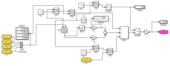
Figure 5.
Simulation model of SMC in MATALB/Simulink.
4.3. Optimal Tuning of the Switching Function Based on GA
As a GA is an efficient optimization method in solving complex problems of high-multimodal, multi-dimensionality, nonlinear, discrete, and discontinuous characters, it has been widely used in engineering fields in the past few years [23]. Thus, a GA is applied in this paper to optimize five parameters () of the SMC controller. Based on the maximum of the fitness function, a GA can find the optimal control gain automatically, such that the control system performance is closer to the expected value [33].
Penalty function methods have been widely used in GAs for constrained optimization problems in the last few years. This method transforms the constrained optimization problem into an unconstrained one by penalizing the objective function corresponding to the infeasible solution [34]. According to the given constraints in Section 4.1 and Section 4.2, the penalty function is given in Equation (22):
The objective function proposed in Equation (6) could reflect the performance of the optimized results. The smaller the value of , the better the control performance of the OSMC controller. Hence, the fitness function is defined based on , which is shown below:
When the fitness function reaches the maximum, the OSMC controller has the best control results, and then the five parameters () of the OSMC controller are optimal. The procedures of a GA in the present study are illustrated in Figure 6.
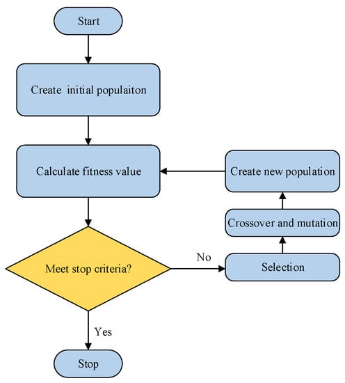
Figure 6.
Working mechanism flowchart of the GA.
Step1. The initial population is created based on the binary coding rules.
Step2. Calculate the corresponding fitness values using Equation (23). Individuals are selected according their fitness value. Those individuals with maximum fitness are copied to the next generation.
Step3. Once the iteration criterium is satisfied, the GA optimization is concluded; otherwise, the next step is conducted.
Step4. A new generation of individuals (i.e., selection) is obtained through the application of genetic operators (i.e., crossover, mutation).
Step5. The GA algorithm concludes once the maximum number of generations is reached. Otherwise, repeat step 4.
The parameters related to the GA-based optimization algorithm are shown in Table 2.

Table 2.
Parameters related to the GA-based optimization algorithm.
For the purpose of reducing the optimization time, the ranges of OSMC parameters are selected based on Equations (16)–(18) and Table 3 as follows.

Table 3.
The actual parameters of the quarter suspension system.
The relationship between genetic algebra and the fitness function values in the process of GA optimization based on MATLAB/Simulink (version 2014a) is shown in Figure 7, and the optimized results are shown in in Section 5.
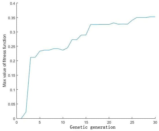
Figure 7.
The relationship between the fitness function value and the generation.
5. Simulations and Analysis
In order to verify the control performance of the OSMC controller optimized by the GA, the models of the passive suspension system and the active suspension system with SMC controller were also built in MATLAB/Simulink. The model of the whole system is shown in Figure 8, and the related parameters of the whole system used in simulations are listed in Table 3.
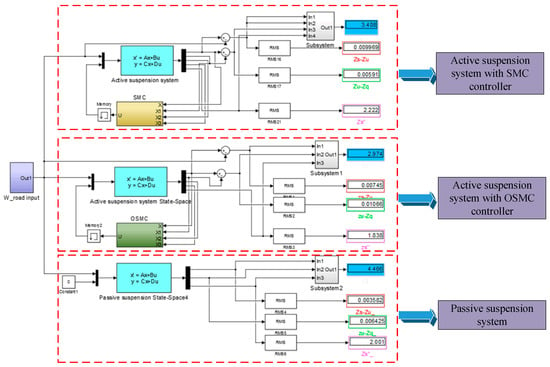
Figure 8.
The whole simulation model of three suspension systems.
The values of were obtained through the GA proposed in Section 4.3 based on the other values in Table 3. The values of and are cited from Reference [35], which is obtained based on the analytic hierarchy process method.
For the passive suspension system, its parameters () are the same as the quarter active suspension system. For the active suspension system with an SMC controller, the related values of the SMC controller were , which are quoted from Reference [36]. The optimal parameters () of Table 3 were put into the OSMC controller. In other words, the state equations of the three suspension systems are the same, the only difference is the control strategy.
Based on the above conditions, the simulations based on MATLAB/Simulink were carried out, and the simulation results are listed from Figure 9, Figure 10, Figure 11 and Figure 12.
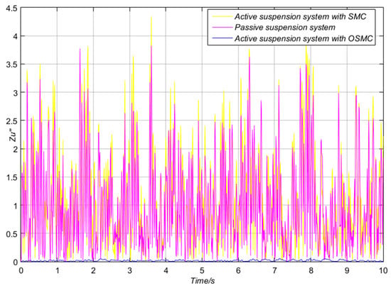
Figure 9.
Comparison of the three suspension systems’ vertical acceleration.
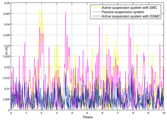
Figure 10.
Different wheel hops of the three suspension systems.
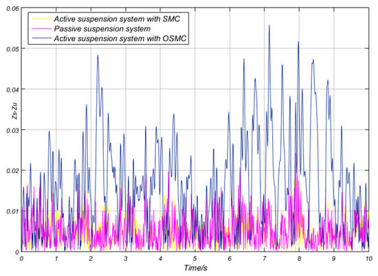
Figure 11.
Vehicle body displacements of the three suspension systems.
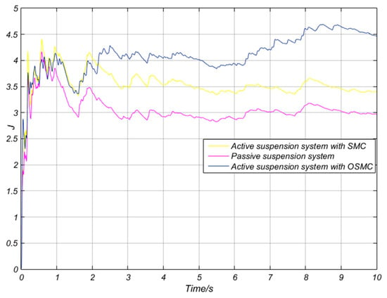
Figure 12.
Performance index J of the three suspension systems.
Based on the curves shown from Figure 9, Figure 10, Figure 11 and Figure 12, the indicators of the active suspension system with an OSMC controller, SMC controller, and passive suspension system can be clearly analyzed. In the aspects of vertical acceleration , the active suspension systems excelled over the passive system, and the OSMC controller performed significantly better than the SMC controller in the active suspension system.
For a better comparison of the indexes of the three suspension systems, the root mean square (RMS) values of indicators are listed in Table 4. As shown in Table 4, the vertical acceleration of the OSMC controller decreased 17.28% and 8.1% more than the SMC controller and passive systems, respectively. The comprehensive performance index of OSMC controller decreased 12.73% and 33.4% more than the SMC controller and passive systems, respectively. The vertical acceleration of the sprung mass is the most important riding comfort performance index [7,8,9]. As a result, the OSMC controller performed better than others in the aspect of riding comfort. As can be seen from Figure 10 and Figure 11 and Table 4, the differences of and among the three suspension systems was significantly small, which indicated that the vehicle stability and the suspension rattle space were almost the same.

Table 4.
Comparisons of three systems about performance indexes.
According to the above analyses, we can come to the conclusion that the active suspension system with the OSMC controller had better performance than that of the SMC controller and the passive suspension system.
In order to demonstrate the validity of the OSMC controller proposed in this paper, two active suspensions mentioned in References [7,9] were optimized, and the results are shown in Figure 13 and Figure 14, respectively.
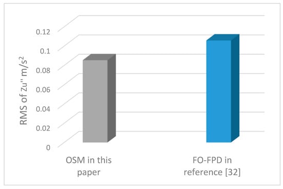
Figure 13.
Comparison of optimum results of two controllers.
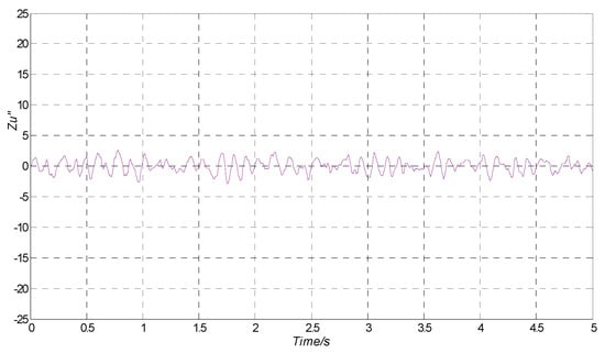
Figure 14.
Optimum vertical acceleration of Reference [9] based on the OSMC controller.
As shown in Figure 13, the RMS of the vertical acceleration decreased 19.34% compared with the optimum results in Reference [7] based on the OSMC controller. The optimized results in Reference [9] are shown in the form of figures, and the optimum vertical acceleration with the OSMC controller are exhibited in Figure 14. Comparing with the vertical acceleration figure in Reference [9], it can be found from Figure 14 that the maximum amplitude was smaller, which means that the OSMC controller performed better.
6. Conclusions
This paper proposed an OSMC controller that is used to control the active suspension system for better ride control. Furthermore, a GA is applied to optimize the SMC switching function and the parameters of the control law (exponential reaching law) to achieve the best control performance that minimizes the objective function. Models of three different suspension systems were established in this paper, and the simulations based on MATLAB/Simulink were performed. The simulation results revealed that the comprehensive performance index of the OSMC controller decreased 12.73% and 33.4% over the SMC controller and the passive system, respectively. We can draw the conclusion that the OSMC controller based on a GA has a better control effect than the traditional SMC controller and the passive suspension system. Moreover, the comparison between the OSMC controller and other controllers mentioned in References [7,9] demonstrate that the OSMC controller proposed in this paper had better performance.
Author Contributions
C.Z. and W.C. conceived and designed the proposed approach; F.X. performed the simulations; C.Z. and X.L. verified the proposed approach; C.Z. wrote the manuscript; C.Z., X.L., and B.C. revised the manuscript.
Funding
This research was funded by The National Key Research and Development Program of China under Grant No. 2016YFC0802904.
Acknowledgments
The authors would like to acknowledge the Institute of Electrohydraulic Control Technology for Engineering Machinery in Jilin University and Xuzhou Construction Machinery Group Co., Ltd., which support this research.
Conflicts of Interest
The authors declare no conflict of interest.
References
- Cui, M.; Geng, L. Random Modeling and Control of Nonlinear Active Suspension. Math. Probl. Eng. 2017, 2017, 4045796. [Google Scholar] [CrossRef]
- Su, X. Master-Slave Control for Active Suspension Systems with Hydraulic Actuator Dynamics. IEEE Access 2017, 5, 3612–3621. [Google Scholar] [CrossRef]
- Mohammadi, Y.; Ganjefar, S. Quarter car active suspension system: Minimum time controller design using singular perturbation method. Int. J. Control Autom. Syst. 2017, 15, 2538–2550. [Google Scholar] [CrossRef]
- Wang, P.; Wang, Q.; Xu, X.; Chen, N. Fractional Critical Damping Theory and Its Application in Active Suspension Control. Shock Vib. 2017, 2017, 2738976. [Google Scholar] [CrossRef]
- Huang, Y.; Na, J.; Wu, X.; Gao, G. Approximation-Free Control for Vehicle Active Suspensions with Hydraulic Actuator. IEEE Trans. Ind. Electron. 2018, 65, 7258–7267. [Google Scholar] [CrossRef]
- Bououden, S.; Chadli, M. A robust predictive control design for nonlinear active suspension systems. Asian J. Control 2016, 18, 122–132. [Google Scholar] [CrossRef]
- Kumar, V.; Rana, K.P.S.; Kumar, J.; Mishra, P. Self-tuned robust fractional order fuzzy PD controller for uncertain and nonlinear active suspension system. Neural Comput. Appl. 2018, 30, 1827–1843. [Google Scholar] [CrossRef]
- Deepika, D.; Narayan, S.; Kaur, S. Robust finite time integral sliding mode tracker for nth-order non-affine non-linear system with uncertainty and disturbance estimator. Math. Comput. Simul. 2018, 156, 364–376. [Google Scholar] [CrossRef]
- Bharali, J.; Garg, N. Efficient Ride Quality and Road Holding Improvement for Active Suspension System. In Proceedings of the 14th IEEE India Council International Conference (INDICON), Roorkee, India, 15–17 December 2017. [Google Scholar]
- Torchani, B.; Sellami, A.; Mhiri, R.; Gareia, G. Study of Comparative Saturated Sliding Mode Control and LQR Controller. J. Mech. Eng. Autom. 2011, 1, 245–249. [Google Scholar]
- Ayadi, A.; Smaoui, M.; Aloui, S. Adaptive sliding mode control with moving surface: Experimental validation for electropneumatic system. Mech. Syst. Signal Process. 2018, 109, 27–44. [Google Scholar] [CrossRef]
- Mohamed, G.; Sofiane, A.A.; Nicolas, L. Adaptive super twisting extended state observer based sliding mode control for diesel engine air path subject to matched and unmatched disturbance. IEEE Trans. Ind. Electron. 2018, 65, 6901–6911. [Google Scholar] [CrossRef]
- Benamor, A.; Messaoud, H. Robust adaptive sliding mode control for uncertain systems with unknown time-varying delay input. ISA Trans. 2018, 79, 1–12. [Google Scholar] [CrossRef]
- Devika, K.B.; Thomas, S. Sliding mode controller design for MIMO nonlinear systems: A novel power rate reaching law approach for improved performance. J. Frankl. Inst. Eng. Appl. Math. 2018, 355, 5082–5098. [Google Scholar]
- Ozer, H.O.; Hacioglu, Y.; Yagiz, N. High order sliding mode control with estimation for vehicle active suspensions. Trans. Inst. Meas. Control 2017, 40, 1457–1470. [Google Scholar] [CrossRef]
- Amini, M.R.; Shahbakhti, M.; PanA, S. Daptive Discrete Second-Order sliding mode control with Application to Nonlinear Automotive Systems. J. Dyn. Syst. Meas. Control. 2018, 140, 121010. [Google Scholar] [CrossRef]
- Liu, J. Simulation of Sliding Mode Control Based on MATLAB; Tsinghua University Press: Beijing, China, 2015; pp. 4–25. [Google Scholar]
- Tuan, L.A.; Cuong, H.M.; van Trieu, P. Adaptive neural network sliding mode control of shipboard container cranes considering actuator backlash. Mech. Syst. Signal Process. 2018, 112, 233–250. [Google Scholar] [CrossRef]
- Alves, U.N.L.; Garcia, J.P.F.; Teixeira, M.; Garcia, S.C.; Rodrigues, F.B. Sliding mode control for active suspension system with data acquisition delay. Math. Probl. Eng. 2014, 2014, 529293. [Google Scholar] [CrossRef]
- Yuvapriya, T.; Lakshmi, P.; Rajendiran, S. Vibration suppression in full car active suspension system using fractional order sliding mode controller. J. Braz. Soc. Mech. Sci. Eng. 2018, 40, 217. [Google Scholar] [CrossRef]
- Repecho, V.; Biel, D.; Olm, J.M. Robust sliding mode control of a DC/DC Boost converter with switching frequency regulation. J. Frankl. Inst. 2018, 355, 5367–5383. [Google Scholar] [CrossRef]
- Ahmadi, M.A.; Zendehboudi, S.; Dusseault, M.B. Evolving simple-to-use method to determine water–oil relative permeability in petroleum reservoirs. J. Pet. 2016, 2, 67–78. [Google Scholar] [CrossRef]
- Mitchell, M. An Introduction to Genetic Algorithms; MIT Press: Cambridge, MA, USA, 1996; Volume 32. [Google Scholar]
- Pankaj, R.; Vineet, S.; Om, P. Determination of Stabilizing Parameter of Fractional Order PID Controller Using Genetic Algorithm. Int. J. Comput. Eng. Manag. 2012, 15, 24–32. [Google Scholar]
- Nabavi, S.; Zhang, L. Design and Optimization of Piezoelectric MEMS Vibration Energy Harvesters Based on Genetic Algorithm. IEEE Sens. J. 2017, 17, 7372–7382. [Google Scholar] [CrossRef]
- Gad, S.; Metered, H.; Bassuiny, A.; Ghany, A. Multi-objective genetic algorithm fractional-order PID controller for semi-active magnetorheologically damped seat suspension. J. Vib. Control 2016, 34, 71–80. [Google Scholar] [CrossRef]
- Almeida, J.H.S.; Ribeiro, M.L. Stacking sequence optimization in composite tubes under internal pressure based on genetic algorithm accounting for progressive damage. Compos. Struct. 2017, 178, 20–26. [Google Scholar] [CrossRef]
- Koch, G.; Pellegrini, E.; Spirk, S.; Lohmann, B. Design and Modeling of a Quarter-Vehicle Test Rig for Active Suspension Control; Technical Reports on Automatic Control; Lehrstuhl für Regelungstechnik: Garching bei München, Germany, 2010; Volume TRAC-5. [Google Scholar]
- Dong, X.; Zhao, D.; Yang, B.; Han, C. Fractional-order control of active suspension actuator based on parallel adaptive clonal selection algorithm. J. Mech. Sci. Technol. 2016, 30, 2769–2781. [Google Scholar] [CrossRef]
- Wang, D.; Zhao, D.; Gong, M.; Yang, B. Nonlinear Predictive Sliding Mode Control for Active Suspension System. Shock Vib. 2018, 2018, 8194305. [Google Scholar] [CrossRef]
- Wang, J. Design Methods of Holographic Optimal Sliding Mode Controllers for Vehicle Active Suspensions. J. Traffic Transp. Eng. 2016, 3, 72–83. [Google Scholar]
- Aly, M.F.; Nassef, A.O.; Hamza, K. Multi-objective design of vehicle suspension systems via a local diffusion genetic algorithm for disjoint Pareto frontiers. Optim. Eng. 2015, 47, 706–717. [Google Scholar] [CrossRef]
- Tran, H.K.; Nguyen, T.N. Flight Motion Controller Design using Genetic Algorithm for a Quadcopter. Meas. Control 2018, 51, 59–64. [Google Scholar] [CrossRef]
- Gupta, R.K.; Bhunia, A.K.; Roy, D. A GA based penalty function technique for solving constrained redundancy allocation problem of series system with interval valued reliability of components. J. Comput. Appl. Math. 2009, 232, 275–284. [Google Scholar] [CrossRef]
- Shian, C.; Feng, Q. A method to determine the weight coefficient of vehicle suspension LQG control. J. Vib. Shock 2008, 2, 65–68. [Google Scholar]
- Yuan, G.A.O.; Wei, X.U.; Huili, L.A.N. Fuzzy sliding mode control for nonlinear vehicle suspension based on differential geometry. J. Hefei Univ. Technol. (Nat. Sci.) 2014, 3, 266–271. [Google Scholar]
© 2018 by the authors. Licensee MDPI, Basel, Switzerland. This article is an open access article distributed under the terms and conditions of the Creative Commons Attribution (CC BY) license (http://creativecommons.org/licenses/by/4.0/).