Deep Directional Network for Object Tracking

Abstract

Existing object trackers are mostly based on correlation filtering and neural network frameworks. Correlation filtering is fast but has poor accuracy. Although a neural network can achieve high precision, a large amount of computation increases the tracking time. To address this problem, we utilize a convolutional neural network (CNN) to learn object direction. We propose a target direction classification network based on CNNs that has a directional shortcut to the tracking target, unlike the particle filter that randomly finds the target. Our network uses an end-to-end approach to determine scale variation that has good robustness to scale variation sequences. In the pretraining stage, the Visual Object Tracking Challenges (VOT) dataset is used to train the network for learning positive and negative sample classification and direction classification. In the online tracking stage, the sliding window operation is performed by using the obtained directional information to determine the exact position of the object. The network only calculates a single sample, which guarantees a low computational burden. The positive and negative sample redetection strategies can successfully ensure that the samples are not lost. The one-pass evaluation (OPE) evaluation results of the object tracking benchmark (OTB) demonstrate that the algorithm is very robust and is also faster than several deep trackers.

1. Introduction

Object tracking is an important part of computer vision. Object tracking has various applications, such as video surveillance, human–computer interaction and traffic monitoring. Therefore, object tracking technology has rapidly advanced in recent years. There are two primary current trends in object tracking: deep learning and correlation filtering. Without the support of large-scale datasets, the potential of deep learning in object tracking has not been developed. Naiyan Wang proposed the DLT [1] algorithm to introduce deep learning to this field for the first time. At that time, because there were no large-scale datasets dedicated to tracking, offline training of DLT was performed using the Tiny Images dataset [2]. This was the first time the researchers observed the effectiveness of deep learning. With the advent of large-scale video sequence datasets, such as VOT (Visual Object Tracking Challenges) [3] and OTB (Visual Tracking Benchmark) [4], a large number of effective deep learning algorithms such as MDNet [5] has emerged, and the use of deep learning in the field of tracking has grown explosively.

Object tracking is a difficult task because of several challenging factors, such as illumination variation (IV), scale variation (SV), occlusion (OCC), deformation (DEF), motion blur (MB), fast motion (FM), in-plane rotation (IPR), out-of-plane rotation (OPR), out-of-view (OV), background clutter (BC) and low resolution (LR) [3]. Traditional object tracking algorithms mostly use artificial features. Artificial features, such as CN (Color Name) [6] and HOG (Histogram of Oriented Gradient) [7], cannot obtain deep semantic information of the object, are not sufficiently robust and are ineffective in overcoming challenges in object tracking. Certain correlation filtering trackers, such as C-COT [8], also abandoned traditional artificial features and turned to deep features that better express the target semantic information. Certain algorithms, e.g., CFNet [9] and DCFNet [10], even entirely abandoned correlation filtering, using CNN’s convolution calculation instead of correlation calculations, and train a correlational deep network model to achieve tracking ability.

The deep convolutional neural network (CNN) has been widely used not only in target detection, such as YOLO [11] but also recently in the field of object tracking. Compared to traditional features, a deep feature can express the semantic information of the target at a deeper level. Presently, deep learning object tracking algorithms primarily use offline training and online fine-tuning for network learning. However, due to the scarcity of computing resources, numerous network parameters and large computational complexity, most deep-learning target tracking algorithms are slow. Similarly, to the MDNet [5] algorithm, most deep learning tracking algorithms use particle sampling mechanisms during the tracking phase to determine the maximum probability of a positive sample strategy for target tracking, undoubtedly increasing the amount of network computation. In the field of object tracking, in a broad sense, a positive sample is the object we need to track, and a negative sample is the background information surrounding the target. But different algorithms will have different positive and negative sample criteria.

The GOTURN [12] algorithm only uses offline training. During the online tracking phase, the frozen network weights are not updated. The search area of the current frame and the target position of the previous frame are input into the network. The network learns to compare these areas to find the target object in the current frame; however, this algorithm can no longer retrieve the target once the target has been lost. At that point, the background will be falsely tracked. In terms of scaling, DSST [13] requires not only a position filter but also a scalar filter. The training of multiple filters undoubtedly increases the complexity of the algorithm.

Inspired by the above observations, we propose a novel deep direction network for object tracking that classifies positive samples into 11 direction and scale categories: upper-left, left, lower-left, lower, lower-right, right, upper-right, upper, small-scale, large-scale and true-sample. We use end-to-end training, and the final output layer of the network has two branches. One branch classifies positive samples into 11 direction categories, and the other classifies positive and negative samples. To enable the network to learn the ability to describe the difference between target and background and to judge whether the target is lost in the tracking phase, the existence of the second branch is necessary. In the tracking phase, the network obtains the information on target direction according to the single sample extracted from the previous position and uses the sliding window operation to approach the target. Our algorithm uses a single-sample tracking strategy, thereby reducing the computational burden on the network and improving the tracking speed. Our algorithm cleverly classifies the target’s positive sample into 11 categories, uses the constraint box size to limit 11 classes, and uses a deep network to learn the differences between categories. Using a deep network can better describe the target and improve the robustness of tracking. Another interesting aspect of our algorithm is that we design a sliding window mechanism for direction classification network.

In summary, we make the following contributions:

• We propose a network for the classification of target direction based on CNNs, and this network has a good adaptability to target tracking.
• Our network successfully incorporates scale variation in a deep network that is robust to scale variation sequences.
• In the online tracking stage, the network only calculates a single sample, which guarantees a low computational burden on the network.
• The positive and negative sample redetection strategies can successfully ensure that the samples are not lost.

The rest of the paper is organized as follows. Section 2 briefly summarizes our related studies. Section 3 describes our direction network mechanism. Section 4 illustrates our online tracking implementation. Section 5 demonstrates our experimental results with direction network in the Visual Tracker Benchmark.

2. Related Work

2.1. Object Tracking Overview

Object tracking is one of the basic components of computer vision and has been studied extensively. It is generally accepted that target tracking is divided into two major categories: discriminative approaches [14,15] and generative approaches [16,17]. The generation method models the target area in the current frame and finds the most similar area in the next frame as the predicted position. Generative models that have been proposed include sparse representation [18], subspace learning [16], etc. Discriminative methods use the target region as the positive sample in the current frame and the background region as the negative sample to train the classifiers via P-N learning [19], multiple instance learning [14], correlation filters [20], etc.; finally, these methods use the trained classifier to find the optimal region in the next frame.

In recent years, correlation filters and deep learning algorithms have become mainstream. Naiyan Wang et al. observed that the results of feature extraction would directly influence the accuracy and efficiency of target tracking [21]. Therefore, most of the traditional artificial features cannot meet the complex environmental challenges in target tracking. Using a deep network to extract target features is a feasible solution.

2.2. Deep Networks in Tracking

Deep networks have been introduced into the target tracking field due to the deep feature semantic information description. In 2013, Naiyan Wang used the fully connected network based on a stacked autoencoder to develop the neural network-based target tracking [1]. Due to the lack of training data, the results were unsatisfactory. C-COT [8] uses a deep feature to directly replace the traditional artificial feature that caused C-COT to rank first in the list of VOT2016 challenge. Convolutional neural networks have been introduced to be more suitable for processing image problems. With the advent of large-scale video tracking datasets, such as VOT [3] and OTB [4], deep learning has a wide range of applications in target tracking [5,22,23]. However, the deep network’s powerful capabilities arise from the large number of parameters and computational power of such networks. Many excellent tracking algorithms that use deep networks cannot be very fast. As an improved version of C-COT [8], ECO [24] aims to improve time and space efficiency. Although MDNet [5] tracking is very effective, the multi-instance mechanism makes the speed slow. In contrast to MDNet [5], we propose a single sample tracking mechanism to track the target, thus reducing the amount of network computing.

3. Direction Deep Network Tracker

Deep networks have great learning potential. Most of the deep learning tracking algorithms extract the deep features of the target for classification and consider the positive sample, which is the most similar to the target as the tracking result. Many deep learning tracking algorithms do not fully utilize the large amount of information of the target sample, and the learning ability of deep networks has not been fully exploited. Therefore, we propose a novel direction deep network that uses directional information designed to classify positive samples more precisely, and according to the directional category of the sample, use the sliding window to find the target faster.

3.1. Overall Framework

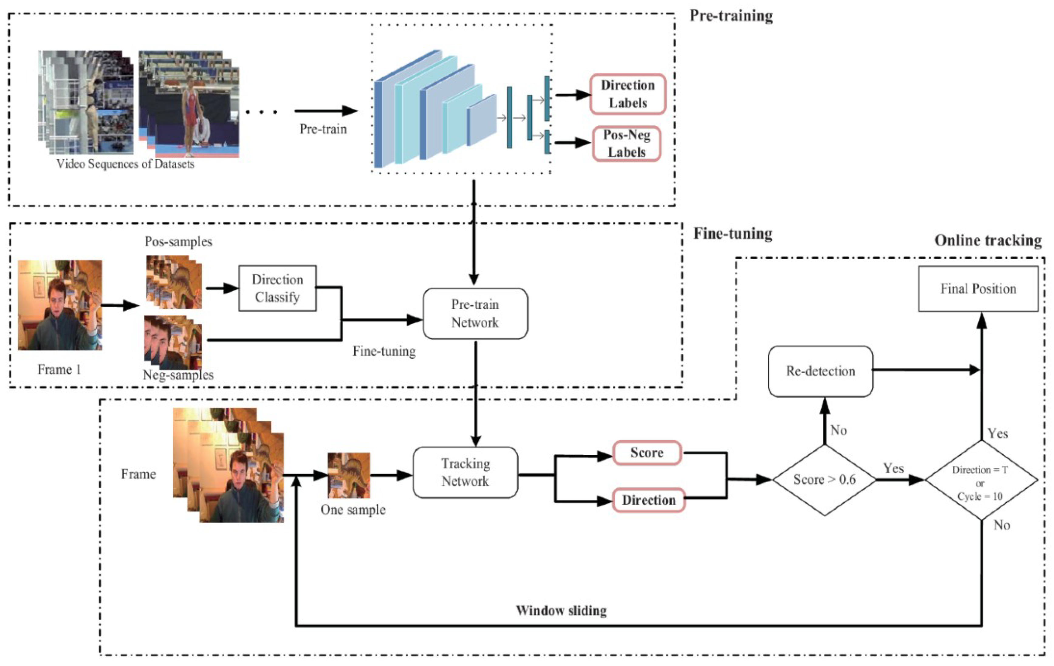
Figure 1 shows the overall flow chart of the tracking algorithm in this paper, including pretraining, fine-tuning and online tracking stages. At the top of the picture is the pretraining phase. The network is pretrained using the specific tracking datasets. Direction labels indicate the category labels for 11 direction categories, and Pos–Neg Labels denote the category labels for positive and negative samples. We obtain a pretrained network and then use the first frame to fine-tune the network. In the fine-tuning phase, we first extract the positive and negative samples. Then, we classify the positive samples into direction categories and fine-tune the network. In the tracking phase, we extract a sample at the previous frame and input the sample into the fine-tuned network to obtain a score and a direction. If the sample is negative, we use the redetection mechanism to determine the final target position. If it is a positive sample, we determine whether the direction class is T (true-sample). If direction class is T, then we obtain the final target position. If it is not, we will perform window sliding to continue sampling. If the number of sliding windows reaches ten, we stop the sliding window operation to determine the final target position.

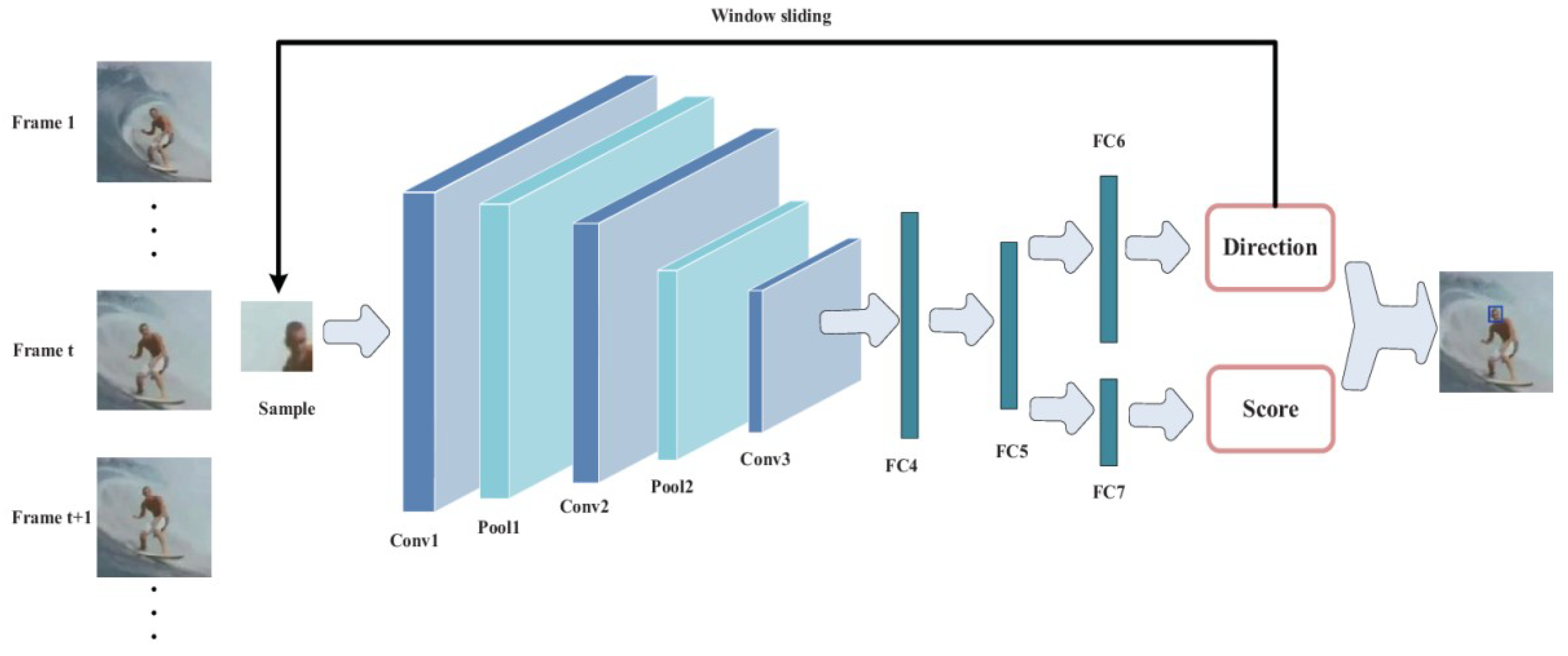
The architecture of the direction of the deep network for target tracking proposed in this paper is shown in Figure 2. The architecture of the network mainly includes three convolutional layers (Conv1, Conv2 and Conv3) and three fully connected layers (FC4, FC5 and {FC6, FC7}). FC6 and FC7 are two independent branches of the same fully connected layer. They represent the direction classification layer and the pos–neg sample classification layers, respectively. There is a pooling layer behind layers conv1 and conv2, denoted Pool1 and Pool2, respectively. In the tracking phase, we extract a sample and then send it to the network to obtain the sample’s direction and score. Direction represents the sample direction category and score represents the pos-neg sample score of the sample. We perform the corresponding sliding window operation according to direction. We judge the final target position according to direction and score.

Table 1. Architecture of the convolutional embedding function.

Input	Layers	Size	Number
112 × 112 × 3	Conv1	7 × 7	96
53 × 53 × 96	Pool1	3 × 3
26 × 26 × 96	Conv2	5 × 5	256
11 × 11 × 256	Pool2	3 × 3
5 × 5 × 256	Conv3	3 × 3	512
3 × 3 × 512	FC4	3 × 3	512
1 × 1 × 512	FC5	1 × 1	512
1 × 1 × 512	FC6	1 × 1	11
1 × 1 × 512	FC7	1 × 1	2

shows the filter sizes and the numbers of each type of layer in the deep directional network. Our network uses three convolutional layers. Our original intention is to reduce computation amount of the network. Too many layers will inevitably increase the amount of computations and too few layers will be difficult to obtain the deep semantic features of the target. So we use three convolutional layers and three fully connected layers. We use the Relu activation function after each convolutional layer and fully connected layer, as shown in Equation (1).

$$Relu\left(x\right)=\{\begin{array}{c}xifx>0\\ 0ifx\le 0\end{array}$$

(1)

3.2. Direction Classification Network

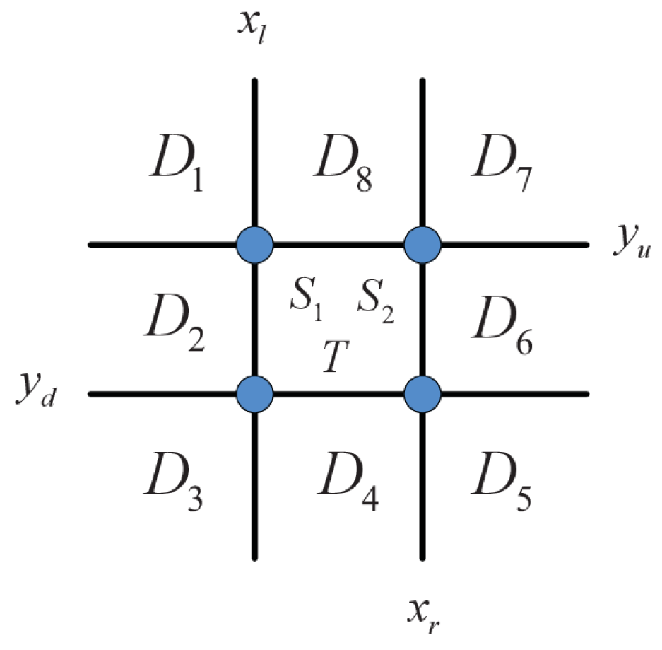
First, we classify positive samples into 11 categories based on direction information, as shown in Figure 3. Specially, the positive samples are divided into upper-left ($D_1$), left ($D_2$), lower-left ($D_3$), lower ($D_4$), lower-right ($D_5$), right ($D_6$), upper-right ($D_7$), upper ($D_8$), small-scale ($S_1$), large-scale ($S_2$) and true-sample (T), namely, 11 classes of direction information.

In Figure 3, $[x_l,x_r,y_u,y_d]$ represents the left boundary, the right boundary, the upper boundary, and the lower boundary, respectively, of the direction division. The setting of the boundary is determined by the size of the original target of the sample, as shown in Equations (2) and (3). Assume that the ground truth of the current frame is represented by ${\mathrm{g}}_t=[x_t,y_t,w_t,h_t]$, where $x_t$ denotes the position of object along the x axis, $y_t$ is the position of object along the y axis coordinate, $w_t$ represents the width of the target along the x axis, and $h_t$ is the height of the target along the y-axis.

$$x_i=\{\begin{array}{c}{x}_t-\alpha w_{t}if\left(i=l\right)\\ x_t+\alpha w_{t}if\left(i=r\right)\end{array}$$

(2)

$$y_j=\{\begin{array}{c}{y}_t-\alpha h_{t}if\left(j=u\right)\\ y_t+\alpha h_{t}if\left(j=d\right)\end{array}$$

(3)

In Equations (2) and (3), $\alpha$ is the scaling factor of the limited boundary; its specific value is described in the experimental section. The category of sample shown in Figure 3 will be determined by the limited boundary in Equations (2) and (3).

$$c=\rho \left({\mathrm{g}}_s,\left[x_l,x_r,y_u,y_d\right],\left[w_t,h_t\right]\right)$$

(4)

Equation (4) describes a mechanism for determining the sample category, where ${\mathrm{g}}_s=[x_s,y_s,w_s,h_s]$ is the positional information of the sample, and $c$ is the output result of the category the sample belongs to. In the paper, $\rho$ is the discriminant function. We use the bounding box $[x_l,x_r,y_u,y_d]$ and sample location information ${\mathrm{g}}_s$ to determine the direction category of the sample, and use $\left[x_l,x_r,y_u,y_d\right]$, ${\mathrm{g}}_s$ and the target’s true width and height $\left[w_t,h_t\right]$ to determine the scale variation category of the sample.

$$c=\{\begin{array}{cc}{D}_1\hfill & \hfill if(x_s\le x_{l}and{y}_s\le y_u)\\ D_2\hfill & \hfill if(x_s\le x_{l}and{y}_u<y_s\le y_d)\\ D_3\hfill & \hfill if(x_s\le x_{l}and{y}_s>y_d)\\ D_4\hfill & \hfill if(y_s\ge y_{d}and{x}_l<x_s\le x_r)\\ D_5\hfill & \hfill if(y_s\ge y_{d}and{x}_s>x_r)\\ D_6\hfill & \hfill if(x_s\ge x_{l}and{y}_u\le y_s\le y_d)\\ D_7\hfill & \hfill if(x_s\ge x_{r}and{y}_s<y_u)\\ D_8\hfill & \hfill if(y_s\le y_{u}and{x}_l<x_s<x_r)\end{array}$$

(5)

The sampling rule will be introduced in Section 3.4 and Section 4. The sample category is determined according to the area corresponding to the sample horizontal and vertical coordinate values, as described in Equation (5). If the sample’s horizontal and vertical coordinates are in the area between the limited boundary, we will judge whether the target scale variation exists. A comparison of $\left[w_s,h_s\right]$ of the sample and the original target truth value $\left[w_t,h_t\right]$ is used to determine the category of scale variation as shown in Equation (6). The traditional scale processing mechanism primarily adopts samples of multiple scales, and the deep network determines which scale is the closest to the target [14]. In contrast to the traditional mechanism, we integrate the scale variation into the sample classification and directly output the scale decision on the classification layer of the deep network, which significantly relies on the strong learning ability of the deep convolutional neural network. The premise of determining the sample scale variation is that the sample coordinates are in the middle of the limited boundary, which is $x_l<x_s<x_r$ and $y_d<y_s<y_u$. The scale decision is primarily determined by Equation (6). The variables $\mathsf{\gamma }$ and $\mathsf{\lambda }$ represent the scale reduction factor and scale enlargement factor, respectively; the specific values will also be introduced in the experimental part. If the sample coordinates are in the bounding box, and there is no scale variation, we classify the sample as belonging to category $\mathrm{T}$.

$$c=\{\begin{array}{c}{S}_{1}if(w_s<\gamma w_{t}or{h}_s<\gamma h_t)\\ S_{2}if(w_s>\gamma w_{t}or{h}_s>\gamma h_t)\end{array}$$

(6)

The specific directional information classification proposed in this paper is described above. The sample classification results subsequently determine the sliding trend of the sliding window network.

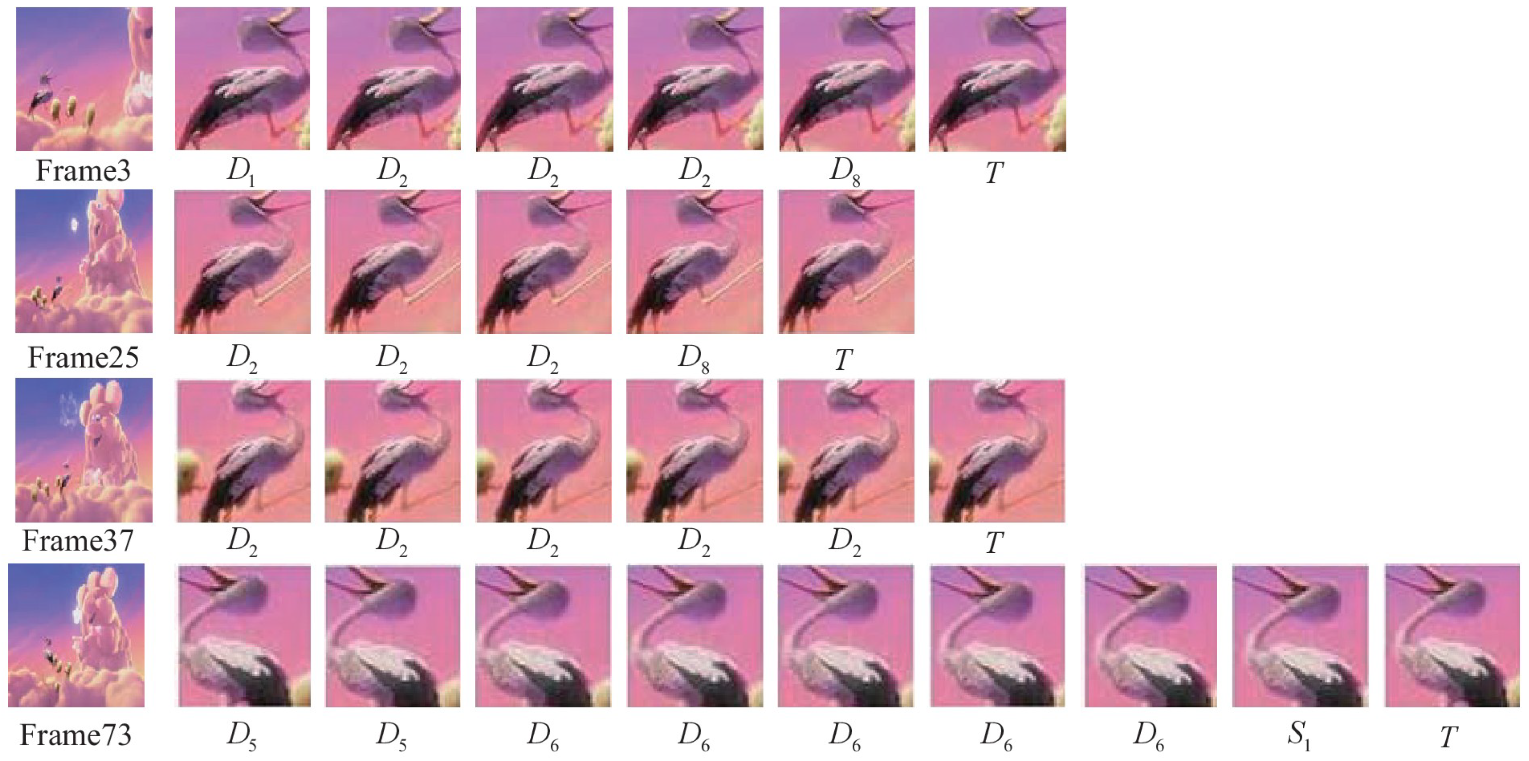
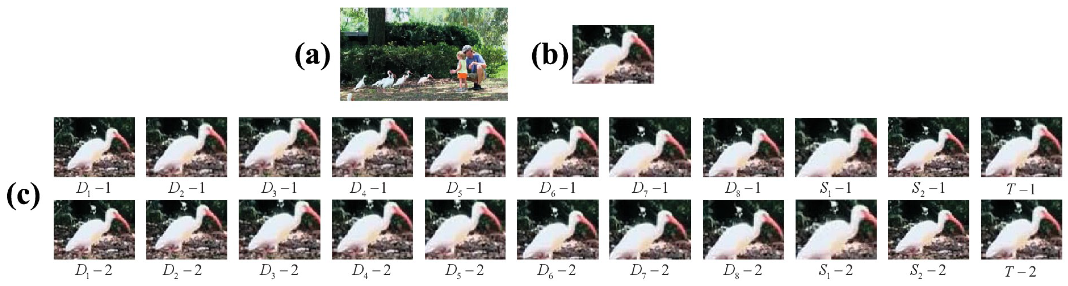
The final classification results of the sample are shown in Figure 4. Two samples are extracted from each class. The original frame is shown in subfigure (a). The sample is from the birds2 video sequence of the VOT2015 [25] dataset. The ground truth of the object is shown in subfigure (b). The category of the sample in subfigure (c) is shown underneath each image of (c). Figure 4 shows that the gap between each sample is very small, almost a pixel-level change; however, each sample has a direction trend of the classification. The final result shows that a powerful neural network can fully learn the small changes in this strategy and classify positive samples accurately.

3.3. Sliding Window Model

Classifying the object sample by the classification network is not the final result of object tracking. When obtaining the sample direction information, a decision network is needed to determine how the sample slowly approaches the true position of the object. This paper uses a sliding window model to gradually approach the ground truth of the object. The sample of the current position is sent to the direction classification network to obtain the current direction class relative to the truth object. According to the direction information, the current sample window is correspondingly swept toward the target. This is the primary idea of the sliding window operation model in this paper.

$${\mathrm{g}}_{s+1}=\{\begin{array}{ll}\left[x_s+\theta ,y_s+\theta ,w_s,h_s\right]& if\left({\mathrm{g}}_s\in D_1\right)\\ \left[x_s+\theta ,y_s,w_s,h_s\right]& if\left({\mathrm{g}}_s\in D_2\right)\\ \left[x_s+\theta ,y_s-\theta ,w_s,h_s\right]& if\left({\mathrm{g}}_s\in D_3\right)\\ \left[x_s,y_s-\theta ,w_s,h_s\right]& if\left({\mathrm{g}}_s\in D_4\right)\\ \left[x_s-\theta ,y_s-\theta ,w_s,h_s\right]& if\left({\mathrm{g}}_s\in D_5\right)\\ \left[x_s-\theta ,y_s,w_s,h_s\right]& if\left({\mathrm{g}}_s\in D_6\right)\\ \left[x_s-\theta ,y_s+\theta ,w_s,h_s\right]& if\left({\mathrm{g}}_s\in D_7\right)\\ \left[x_s,y_s+\theta ,w_s,h_s\right]& if\left({\mathrm{g}}_s\in D_8\right)\\ \left[x_s,y_s,w_s+\theta ,h_s+\theta \right]& if\left({\mathrm{g}}_s\in S_1\right)\\ \left[x_s,y_s,w_s-\theta ,h_s-\theta \right]& if\left({\mathrm{g}}_s\in S_2\right)\end{array}$$

(7)

The corresponding sliding window strategy for each direction category is described by Equation (7). The specific implementation measures are shown in Equation (7). In the equation, $\theta$ represents the pixel size of the sliding window operation. Variable ${\mathrm{g}}_{s+1}$ indicates the next sample point to be sampled. When the sample of ${\mathrm{g}}_{s+1}$ is classified as belonging to category $T$, which is the closest to the target, the sliding window operation is stopped; finally, the object tracking result of the current frame is obtained.

3.4. Pretrained Direction Network

This paper uses a deep convolutional neural network, as shown in Figure 2 and Table 1. At the end of this network, a directional information classification layer is added to obtain the information on target direction. The previous three convolutional layers of the direction network use VGG-M [26]. Numerous studies have proven that convolutional networks, such as VGG-Net, GoogLeNet [27], etc., trained with large-scale datasets achieve good generalization performance and transfer learning capabilities. Our network uses the network weights that outstanding scholars have trained as the initialization of the direction network, and greatly improves the ability of tracking learning on the network.

The network framework finally adopts a dual-category network, whereby one classification network is trained to learn the direction information, and the other classification network is trained to learn the sample classification. As shown in Figure 2, FC6 is a direction network that can classify eleven types of direction. FC7 is a sample classification network that is used to classify target and background information. We use the softmax cross-entropy loss function, stochastic gradient descent and backpropagation to update the network weights. The number of network pretraining cycles is 100, and the training dataset consists of 58 video sequences from the VOT2013, VOT2014 and VOT2015 datasets. Using video sequences for network pretraining is different from using large-scale classified data in the past. This method is more suitable for the tracking network.

The training samples were selected by the overlap rate strategy. To enable the network to learn more target orientation information during the training phase, the threshold value of the overlap rate is set to a smaller value of 0.6.

$$l=\{\begin{array}{cc}1\hfill & \hfill ifIoU\left({\mathrm{g}}_s,{\mathrm{g}}_t\right)>0.6\\ 0\hfill & \hfill otherwise\end{array}$$

(8)

Positive and negative samples classification and threshold setting are shown in Equation (8), where $l$ represents the label of positive and negative samples, and $IoU$ denotes the calculation of the overlap rate. If the overlap rate of ${\mathrm{g}}_s$ and ${\mathrm{g}}_t$ is greater than 0.6, $l$ is judged to be positive; otherwise, it is negative. The number of samples per frame is set to 200 positive samples and 50 negative samples. The convolutional layer learning rate is 0.0001, and the fully connected layer learning rate is 0.001. The positive samples obtained by Equation (8) are classified as various direction categories according to the decision criterion in the Equation (4).

The direction network is trained by minimizing the multi-task loss function. The multi-task loss function is defined as Equation (9). $m$ donates the batch size, $L$ denotes the cross-entropy loss function. ${\widehat{c}}_i$ and ${\widehat{l}}_i$ represents the predicted direction and class respectively.

$$L_{mt}=\frac{1}{m}{\displaystyle \sum }_{i=1}^{m}L\left(c_i,{\widehat{c}}_i\right)+\frac{1}{m}{\displaystyle \sum }_{i=1}^{m}L(l_i,{\widehat{l}}_i)$$

(9)

4. Online Tracking

After pretraining, we will obtain a deep network with updated weights. However, pretrained networks often cannot be used directly for new video sequences, and a strategy is needed, such as network initialization, online fine-tuning, tracking redetection mechanism, etc.

The pretrained network uses a large number of video sequences and has a good generalization performance. However, the network for specific video sequence tracking also requires fine-tuning. Therefore, in the first frame, the same strategy as pretraining is used to fine-tune the network weight so that the network applies to the video sequence. This algorithm selects 500 positive samples and 200 negative samples to initialize the network in the first frame. The overlap rate is set to 0.7.

The biggest challenge in target tracking is the deformation of the target. When the target moves for a period of time, the deformation will appear as an enlargement or reduction of size. In this case, the network trained by the feature information of the first frame cannot fully describe the target itself, so it is crucial to fine-tune the network online with the target feature of the new location. To solve the above problem, in the online tracking phase, the target is resampled after continuous tracking of 20 frame sequences. The number of samples is 200 positive samples and 50 negative samples, and the overlapping rate remains unchanged. In the online tracking phase, the training mechanism for resampling is similar to the pretraining phase. Our algorithm automatically selects positive and negative samples based on the threshold and the overlap rate as shown in Equation (8). Then, positive samples are automatically divided into 11 categories as shown in Equations (5) and (6). Our algorithm updates the network weights automatically using the resampled data. Fine-tuning the network can improve the network’s ability to deal with various deformations.

The dual-classification network is designed to deal with the loss of the tracking object. In Figure 1, when the positive sample score is less than a certain threshold $\sigma$, the positive sample is determined to have been lost, and the tracking result consists entirely of the background. The value of $\sigma$ will be given in the experimental section. At this time, the particle sampling strategy is adopted. The default target has only a small range of motion in adjacent frames. Then, the current frame is sampled using the Gaussian distribution rule at the previous frame target position, and the number of samples is set to 300. The samples are input into the network, and the sample with the highest score is selected from the positive and negative sample classification layer as the target position of the current frame.

The tracking sliding window strategy is performed at most 10 times per frame, and the loss mechanism is used if the target is not found during the sliding window operation. Experiments show that most frames can find the target after approximately 10 iterations of the sliding window operation. Because the sliding window mechanism makes it unnecessary to extract a large number of samples for each tracking, the computational burden of the deep network is reduced. As a result, the tracking speed of the network has been improved. Our proposed direction deep network tracker successfully tracked the target, as we had expected.

Figure 5 shows a schematic diagram of the sliding window. The video sequence is from the Bird2 sequence of the OTB-100 dataset. The first, second, third and fourth lines represent the tracking procedure diagrams of sliding windows for the 3rd, 25th, 37th and 73th frames, respectively. The label below each figure indicates the direction category of the current sample. We consider the first line as an example to describe the sliding window tracking procedure. The first picture of the first line represents the current frame. The second is the sample at the previous frame target position; we use the direction deep network to obtain the first sample category $D_1$. Then, we use the sliding window to obtain the second sample according to $D_1$, and we use the direction deep network to obtain the second sample category $D_2$, etc. When the sample output of the sixth sliding window is classified as category $T$, it is considered as the tracking result of this frame. Figure 5 shows that the number of samples extracted in each frame of the proposed algorithm is close to 10.

5. Experiment

5.1. Implementation Details

In this paper, VOT2013, VOT2014 and VOT2015 video sequence datasets are used for pretraining. The initial weight of the convolutional layer is from VGG-M [26]. The test standard used in the experiment is the object tracking benchmark (OTB) [4]. Our algorithm is implemented on the MATLAB platform on Windows 10. The network construction uses the MatConvNet toolbox [28]. The hardware platform uses Intel i7 8700K CPU, 8GB of RAM and NVIDIA GTX 750TI GPU. In the pretraining phase, all network weights of the convolutional layer and the fully connected layer are updated, but in the tracking phase, the convolutional layer is only used for feature extraction, and the fully connected layer’s weights are fine-tuned online. Based on a large number of experiments, setting $\alpha$ to 0.06, $\gamma$ to 0.9, $\lambda$ to 1.1, the setting of $\theta$ to 0.9, and $\sigma$ to 0.6 was determined to maximize the robustness of the tracking effect of the entire network.

To better verify the performance of the proposed algorithm, 58 challenging video sequences were selected for experimentation. These video sequences include illumination variation (IV), scale variation (SV), object occlusion (OCC), deformation (DEF), motion blur (MB), fast motion (FM), in-plane rotation (IPR), out-of-plane rotation (OPR), out-of-view (OV), background clutter (BC), low resolution (LR) and other challenges. In the experiment, 7 excellent recent algorithms were selected for comparison: CNT [29], HCF [30], SiamFC [14], SAMF [31], DeepSRDCF [32], CREST [33] and Staple [34]. The following comparison will help us perform a qualitative analysis of the proposed algorithm.

5.2. Comparison of Effects

This paper selects six sequences containing different challenge factors to display the tracking results. Parts of Figure 6 denoted (a), (b), (c), (d), (e) and (f) correspond to sequences Bird2, Bolt, Couple, Football1, Jogging and Human3, respectively.

As shown in Figure 6, sequence (a) Bird2 contains challenge factors such as (OCC, DEF, FM, IPR, OPR), yet the algorithm proposed in this paper can still successfully track it. The algorithm excels not only in tracking accuracy but also in scale processing. Sequence (b) Bolt is includes challenge factors (OCC, DEF, IPR, OPR). Since the beginning of tracking, several algorithms, such as CNT, SAMF and DeepSRDCF, have lost the object, while our algorithm (“Ours”) and SiamFC, CREST and Staple algorithms continued to successfully track it. At the end of the sequence, our algorithm still tracked the object as successfully as most of the state-of-the-art algorithms. Sequences (c), (d) and (e) all contain numerous challenges. The deep direction network tracking still performs well. Tracking sequence (f) Human3 faces challenges such as (SV, OCC, DEF, OPR, BC), but it is observed that the algorithm of this paper performs best. Although the SAMF algorithm can also track the target, the algorithm of this paper has the best scale processing. It is observed from the six sequences that the deep directional network proposed in this paper can successfully overcome various challenges posed by video sequences.

5.3. Evaluation of Object Tracking Benchmark (OTB)

To analyze the overall performance of our algorithm, the one-pass evaluation (OPE) standard of OTB was used for a comparative evaluation.

Figure 7 shows the evaluations of this algorithm and 7 recent excellent algorithms using the OPE standard. Subfigure (a) evaluates the tracking precision, and (b) evaluates the success rate. Figure 7 shows that the algorithm is ranked first in terms of precision and success rate, although it has only a small gap with the algorithm in the second place.

Table 2. Precision and speed comparison of six deep learning tracking algorithms.

Tracker	Precision	FPS
Ours	0.898	6
MDNet	0.909	<1
CREST	0.875	1
C-COT	0.824	1
DeepSRDCF	0.841	<1
CNT	0.543	1.5

shows the precision and the tracking speed denoted by FPS of recent high-performance deep learning-based tracking algorithms. It is observed that the deep learning-based tracking algorithms developed in recent years have high-performance precision but have struggled with slower tracking speeds. Although our algorithm is still not real-time, it has greatly improved the speed compared to that of other high-performance deep networks. Due to the sliding window mechanism of our algorithm, the number of samples is reduced. The amount of computation in the deep network is successfully reduced. Hence, the tracking speed is improved.

Various algorithms will have different effects on videos with different challenges; hence, this paper will also analyze the effect of each algorithm on different challenge factors, as shown in Figure 8. The graph shows the analysis of the effect of the four challenge factors. The effect of each algorithm on the in-plane rotation sequence is shown in Figure 8a,b, in which (33) indicates that 33 video sequences in the experimental sequence belong to in-plane rotation. It is observed that our algorithm deals with in-plane rotation (shown in Figure 8a,b) and scale variation (shown in Figure 8c,d) with the highest precision and success rate. Considering the background clutter (shown in Figure 8e,f), our algorithm performs well in terms of precision and is ranked third by success rate. Each algorithm has its limitations. For motion-blur video sequences shown in Figure 8g,h, the tracking effect of our algorithm has changed dramatically; hence, our algorithm is not suitable for tracking objects in such videos.

6. Conclusions

This paper presents a deep network-based direction tracker. A three-layer convolutional neural network is used to extract the object feature, and three-layer fully connected networks are used to classify samples. We use the direction deep network to obtain the sample direction category. According to the category, the sliding window mechanism slides the sample window to the target direction until it finds the target. Unlike many previous multisample tracking algorithms, our algorithm uses only one sample for each sliding window operation, which reduces the amount of calculations and improves the tracking speed. In case of fast motion and motion blur sequences, our algorithm also adopts a redetection strategy. When the positive sample score is lower than the threshold, we assume that the tracker is tracking background information. Then, we adopt the multisample assessment mechanism used by most deep learning object tracking networks. To improve the tracker’s robustness, we also regularly fine-tune the tracker online. Experiments show that our algorithm has significant advantages over the existing algorithms. However, in cases of motion blur and low-resolution sequences, this algorithm still has its limitations. Future work needs to start from this shortcoming to solve the problem of object tracking.

References

1. Wang, N.; Yeung, D.Y. Learning a deep compact image representation for visual tracking. In International Conference on Neural Information Processing Systems; Curran Associates Inc.: Red Hook, NY, USA, 2013; pp. 809–817. [Google Scholar]
2. Torralba, A.; Fergus, R.; Freeman, W.T. 80 million tiny images: A large data set for nonparametric object and scene recognition. IEEE Trans. Pattern Anal. Mach. Intell. 2008, 30, 1958–1970. [Google Scholar] [CrossRef] [PubMed]
3. Kristan, M.; Pflugfelder, R.; Leonardis, A.; Matas, J.; Porikli, F.; Cehovin, L.; Nebehay, G.; Fernandez, G.; Vojir, T.; Gatt, A.; et al. The visual object tracking vot2013 challenge results. In Proceedings of the 2013 IEEE International Conference on Computer Vision Workshops (ICCVW), Sydney, Australia, 2–8 December 2013. [Google Scholar]
4. Wu, Y.; Lim, J.; Yang, M.H. Online object tracking: A. benchmark. In Proceedings of the 2013 IEEE Conference on Computer Vision and Pattern Recognition (CVPR), Portland, OR, USA, 23–28 June 2013. [Google Scholar]
5. Nam, H.; Han, B. Learning multi-domain convolutional neural networks for visual tracking. In Proceedings of the 2016 IEEE Conference on Computer Vision and Pattern Recognition (CVPR), Las Vegas, NV, USA, 26 June–1 July 2016. [Google Scholar]
6. Danelljan, M.; Shahbaz Khan, F.; Felsberg, M.; Van de Weijer, J. Adaptive color attributes for real-time visual tracking. In Proceedings of the IEEE Conference on Computer Vision and Pattern Recognition (CVPR), Columbus, OH, USA, 24–27 June 2014. [Google Scholar]
7. Dalal, N.; Triggs, B. Histograms of oriented gradients for human detection. In Proceedings of the CVPR 2005 IEEE Computer Society Conference on Vision and Pattern Recognition, San Diego, CA, USA, 20–25 June 2005; Volume 1. [Google Scholar]
8. Danelljan, M.; Robinson, A.; Khan, F.S.; Felsberg, M. Beyond correlation filters: Learning continuous convolution operators for visual tracking. In European Conference on Computer Vision; Springer: Cham, Switzerland, 2016. [Google Scholar]
9. Valmadre, J.; Bertinetto, L.; Henriques, J.; Vedaldi, A.; Torr, P.H. End-to-end representation learning for correlation filter based tracking. In Proceedings of the 2017 IEEE Conference on Computer Vision and Pattern Recognition (CVPR), Honolulu, HI, USA, 21–26 July 2017. [Google Scholar]
10. Wang, Q.; Gao, J.; Xing, J.; Zhang, M.; Hu, W. DCFNet: Discriminant Correlation Filters Network for Visual Tracking. arXiv, 2017; arXiv:1704.04057. [Google Scholar]
11. Redmon, J.; Divvala, S.; Girshick, R.; Farhadi, A. You only look once: Unified, real-time object detection. In Proceedings of the IEEE Conference on Computer Vision and Pattern Recognition (CVPR), Boston, MA, USA, 7–12 June 2015. [Google Scholar]
12. David, H.; Thrun, S.; Savarese, S. Learning to track at 100 fps with deep regression networks. In European Conference on Computer Vision; Springer: Cham, Switzerland, 2016. [Google Scholar]
13. Danelljan, M.; Häger, G.; Khan, F.; Felsberg, M. Accurate scale estimation for robust visual tracking. In Proceedings of the British Machine Vision Conference, Nottingham, UK, 1–5 September 2014. [Google Scholar]
14. Babenko, B.; Yang, M.; Belongie, S. Visual tracking with online multiple instance learning. In Proceedings of the CVPR 2009 IEEE Conference on Computer Vision and Pattern Recognition, Miami, FL, USA, 20–25 June 2009. [Google Scholar]
15. Zhang, K.; Zhang, L.; Yang, M. Fast compressive tracking. IEEE Trans. Pattern Anal. Mach. Intell. 2014, 36, 2002–2015. [Google Scholar] [CrossRef] [PubMed]
16. Ross, D.A.; Lim, J.; Lin, R.S.; Yang, M.H. Incremental learning for robust visual tracking. Int. J. Comput. Vis. 2008, 77, 125–141. [Google Scholar] [CrossRef]
17. Zhang, T.; Bibi, A.; Ghanem, B. In defense of sparse tracking: Circulant sparse tracker. In Proceedings of the IEEE Conference on Computer Vision and Pattern Recognition, Las Vegas, NV, USA, 27–30 June 2016. [Google Scholar]
18. Mei, X.; Ling, H. Robust visual tracking and vehicle classification via sparse representation. IEEE Trans. Pattern Anal. Mach. Intell. 2011, 33, 2259–2272. [Google Scholar] [PubMed]
19. Kalal, Z.; Mikolajczyk, K.; Matas, J. Tracking-learning-detection. IEEE Trans. Pattern Anal. Mach. Intell. 2012, 34, 1409–1422. [Google Scholar] [CrossRef] [PubMed] [Green Version]
20. Henriques, J.F.; Caseiro, R.; Martins, P.; Batista, J. High-speed tracking with kernelized correlation filters. IEEE Trans. Pattern Anal. Mach. Intell. 2015, 37, 583–596. [Google Scholar] [CrossRef] [PubMed]
21. Wang, N.; Shi, J.; Yeung, D.Y.; Jia, J. Understanding and diagnosing visual tracking systems. In Proceedings of the 2015 IEEE International Conference on Computer Vision (ICCV), Santiago, Chile, 7–13 December 2015. [Google Scholar]
22. Wang, N.; Li, S.; Gupta, A.; Yeung, D.Y. Transferring rich feature hierarchies for robust visual tracking. arXiv, 2015; arXiv:1501.04587. [Google Scholar]
23. Nam, H.; Baek, M.; Han, B. Modeling and propagating cnns in a tree structure for visual tracking. arXiv, 2016; arXiv:1608.07242. [Google Scholar]
24. Danelljan, M.; Bhat, G.; Khan, F.S.; Felsberg, M. ECO: Efficient convolution operators for tracking. In Proceedings of the 2017 IEEE Conference on Computer Vision and Pattern Recognition (CVPR), Honolulu, HI, USA, 21–26 July 2017. [Google Scholar]
25. Kristan, M.; Matas, J. The visual object tracking vot2015 challenge results. In Proceedings of the Visual Object Tracking Workshop 2015 at ICCV2015, Santiago, Chile, 7–13 December 2015. [Google Scholar]
26. Chatfield, K.; Simonyan, K.; Vedaldi, A.; Zisserman, A. Return of the devil in the details: Delving deep into convolutional nets. arXiv, 2014; arXiv:1405.3531. [Google Scholar]
27. Szegedy, C.; Liu, W.; Jia, Y.; Sermanet, P.; Reed, S.; Anguelov, D.; Erhan, D.; Vanhoucke, V.; Rabinovich, A. Going deeper with convolutions. In Proceedings of the IEEE Conference on Computer Vision and Pattern Recognition (CVPR), Boston, MA, USA, 7–12 June 2015. [Google Scholar]
28. Vedaldi, A.; Lenc, K. MatConvnet: Convolutional Neural Networks for MATLAB. In Proceedings of the 23rd ACM International Conference on Multimedia, Brisbane, Australia, 26–30 October 2015. [Google Scholar]
29. Zhang, K.; Liu, Q.; Wu, Y.; Yang, M.H. Robust visual tracking via convolutional networks without training. IEEE Trans. Image Process. 2016, 25, 1779–1792. [Google Scholar] [CrossRef] [PubMed]
30. Ma, C.; Huang, J.B.; Yang, X.; Yang, M.H. Hierarchical convolutional features for visual tracking. In Proceedings of the IEEE International Conference on Computer Vision, Santiago, Chile, 7–13 December 2015. [Google Scholar]
31. Li, Y.; Zhu, J. A scale adaptive kernel correlation filter tracker with feature integration. In European Conference on Computer Vision; Springer: Cham, Switzerland, 2014. [Google Scholar]
32. Danelljan, M.; Hager, G.; Shahbaz Khan, F.; Felsberg, M. Convolutional features for correlation filter based visual tracking. In Proceedings of the IEEE International Conference on Computer Vision Workshops, Washington, DC, USA, 7–13 December 2015. [Google Scholar]
33. Song, Y.; Ma, C.; Gong, L.; Zhang, J.; Lau, R.W.; Yang, M.H. Crest: Convolutional residual learning for visual tracking. In Proceedings of the 2017 IEEE International Conference on Computer Vision (ICCV), Venice, Italy, 22–29 October 2017. [Google Scholar]
34. Bertinetto, L.; Valmadre, J.; Golodetz, S.; Miksik, O.; Torr, P.H. Staple: Complementary learners for real-time tracking. In Proceedings of the IEEE Conference on Computer Vision and Pattern Recognition, Las Vegas, NV, USA, 27–30 June 2016. [Google Scholar]
Figure 1. Overall flow chart of our tracking algorithm.
Algorithms 11 00178 g001
Figure 2. Architecture of our direction learning network.
Algorithms 11 00178 g002
Figure 3. Direction map.
Algorithms 11 00178 g003
Figure 4. Sample classification result. (a) Original frame; (b) Ground truth of the object; (c) Category of the sample.
Algorithms 11 00178 g004
Figure 5. Schematic diagram of the sliding window.
Algorithms 11 00178 g005
Figure 6. Eight algorithms for tracking results of various tracking sequences. (a) Bird2 tracking result; (b) Bolt tracking result; (c) Couple tracking result; (d) Football1 tracking result; (e) Jogging tracking result; (f) Human3 tracking result.
Algorithms 11 00178 g006
Figure 7. Precision and success plots on object tracking benchmark (OTB). (a) Precision plots of OPE; (b) Success plots of OPE.
Algorithms 11 00178 g007
Figure 8. Performance evaluation of eight algorithms for different challenge factors. (a) Precision plots of OPE-in-plane rotation; (b) Success plots of OPE-in-plane rotation; (c) Precision plots of OPE-scale variation; (d) Success plots of OPE-scale variation; (e) Precision plots of OPE-background clutter; (f) Success plots of OPE-background clutter; (g) Precision plots of OPE-motion blur; (h) Success plots of OPE-motion blur.
Algorithms 11 00178 g008