Airfoil Optimization Design Based on the Pivot Element Weighting Iterative Method

Abstract

Class function/shape function transformation (CST) is an advanced geometry representation method employed to generate airfoil coordinates. Aiming at the morbidity of the CST coefficient matrix, the pivot element weighting iterative (PEWI) method is proposed to improve the condition number of the ill-conditioned matrix in the CST. The feasibility of the PEWI method is evaluated by using the RAE2822 and S1223 airfoil. The aerodynamic optimization of the S1223 airfoil is conducted based on the Isight software platform. First, the S1223 airfoil is parameterized by the CST with the PEWI method. It is very significant to confirm the range of variables for the airfoil optimization design. So the normalization method of design variables is put forward in the paper. Optimal Latin Hypercube sampling is applied to generate the samples, whose aerodynamic performances are calculated by the numerical simulation. Then the Radial Basis Functions (RBF) neural network model is trained by these aerodynamic performance data. Finally, the multi-island genetic algorithm is performed to achieve the maximum lift-drag ratio of S1223. The results show that the robustness of the CST can be improved. Moreover, the lift-drag ratio of S1223 increases by 2.27% and the drag coefficient decreases by 1.4%.

1. Introduction

Shape parameterization, which can represent the geometries by the coefficients of the parameterization, is a crucial step in the airfoil aerodynamic optimization [1]. The range of the design variables and the order of the parameterization have a significant effect on the design space which can determine the optimum geometries obtainable. Therefore, it is very important for the designer to choose a proper shape parameterization method.

The Bezier polynomial method [2,3], the B-spline method [4], and the class function/shape function transformation method [1,5,6,7,8] are widely used in the airfoil parameterization design. In order to fit the curves of airfoils, the least square method is generally adopted to obtain control parameters in these three methods. The CST method is based on analytical expressions to represent and modify the various shapes [9]. The CST method is widely used in the airfoil aerodynamic optimization.

For the symmetric NACA0012 airfoil and small camber RAE2822 airfoil, the low order Bernstein polynomials (BPO) can reach the requirement of the airfoil fitting accuracy. But for some large camber airfoils, it is necessary to increase the order of Bernstein polynomials. Because the fitting errors of low order Bernstein polynomials are large. Ceze [10] found that the coefficient matrix was obviously ill-conditioned for the 36th Bernstein polynomial of CST. Guan et al. [11,12] analyzed the coefficient matrix of the Bernstein polynomial and found that the higher the order of control parameters of the polynomial was, the worse the mathematic behavior of control parameters was. Wang et al. [13] discovered that the higher the order of the Bernstein polynomial was, the closer the coefficient matrix was to morbidity.

Essentially the parameterization equation of the CST method is a linear equation. The coefficient matrix of the parameterization equation is ill-conditioned in most cases. And the higher the order of the coefficient matrix is, the larger the condition number is. The larger the condition number of the coefficient matrix is, the closer the coefficient matrix is to morbidity. The solution of the linear equation is very sensitive to the preturbations of the coefficient matrix. These preturbations can lead to the inaccurate solution. Therefore, an inaccurate Bernstein coefficient solution of the CST method can be obtained for the morbidity.

Aiming at the ill-conditioned linear equation, Wu et al. [14] proposed a new iterative improvement which was more effective for the ill-conditioned equation. The ill-conditioned problem could be converted into a series of relatively well-conditioned problems. Salkuyeh et al. [15] put forward a new iterative refinement to solve the ill-conditioned problem and the two-step iterative method could refine the ill-conditioned equation.

The CST method is adopted to reproduce the NACA0012, RAE2822, and S1223 airfoils in this paper. When the number of control parameters for the S1223 airfoil increase, the Bernstein coefficient matrix is close to ill-conditioned and the condition number of this matrix increases. The slight fluctuations of the control point coordinates or the Bernstein coefficient matrix can lead to the huge change of Bernstein coefficients. So two similar shape airfoils have entirely different control parameters and it is unfavorable for the global optimization of airfoils to select the control parameters.

The CST with the pivot element weighting iterative method is proposed to improve the ill-conditioned Bernstein coefficient matrix. And the ill-conditioned Bernstein coefficient matrix trends to be well-conditioned. So accurate control parameters can be calculated and the robustness of the CST method is also improved. The range of control parameters has a great influence on the airfoil optimization. Therefore normalization method is put forward to control the range of parameters. Genetic algorithm is adopted in the S1223 airfoil optimization.

2. Airfoil Parameterization

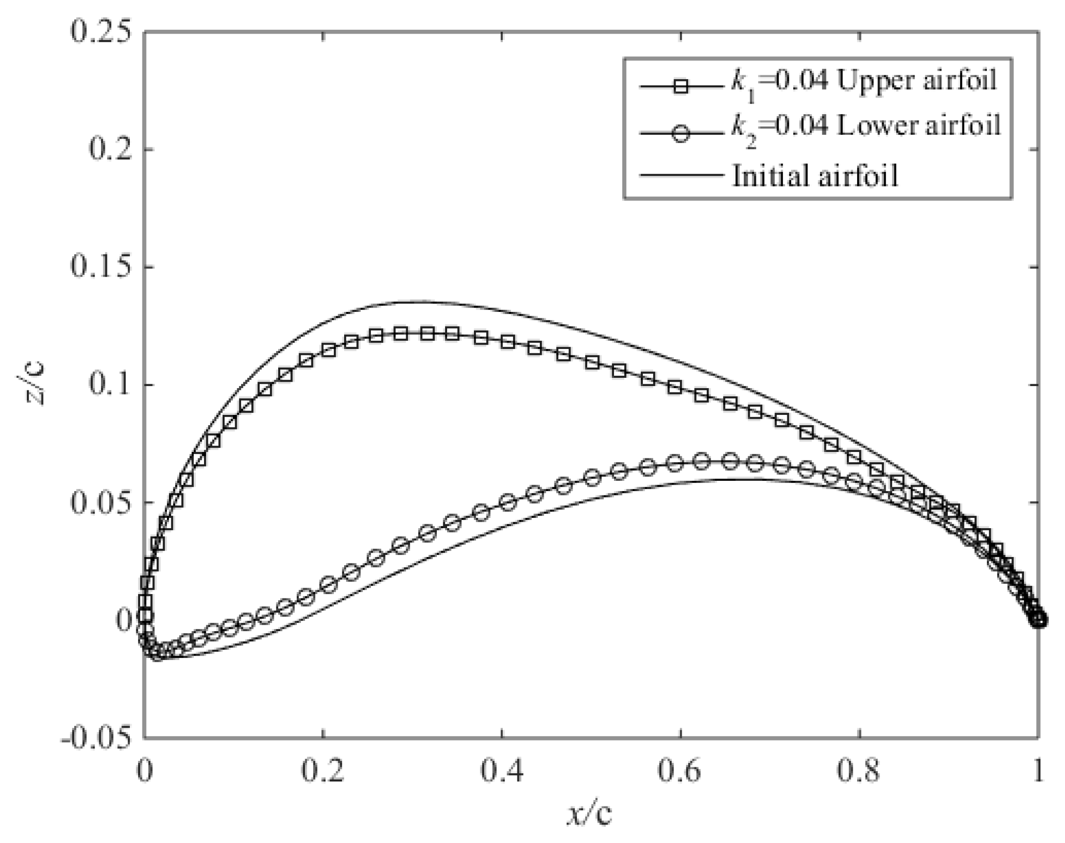
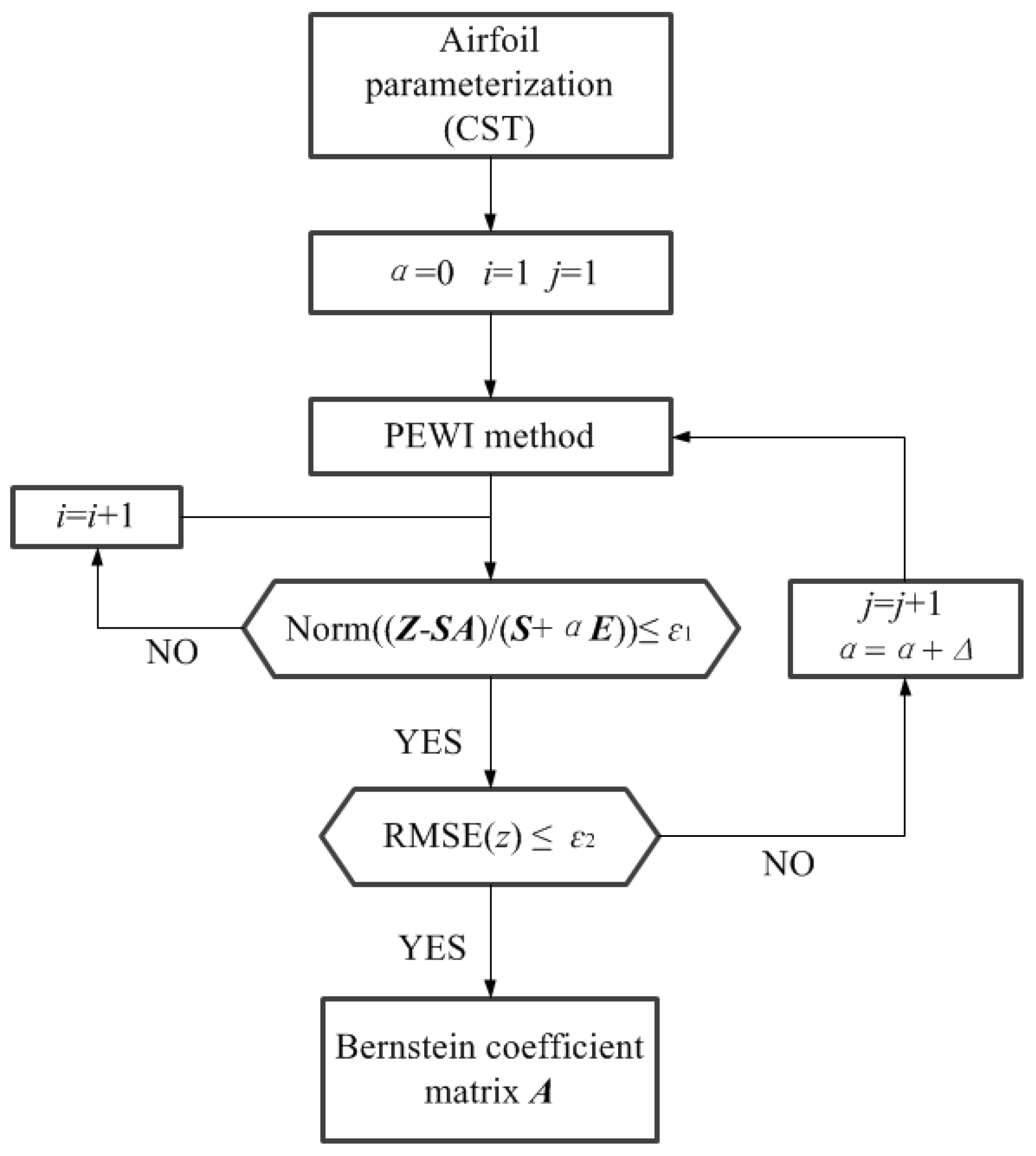
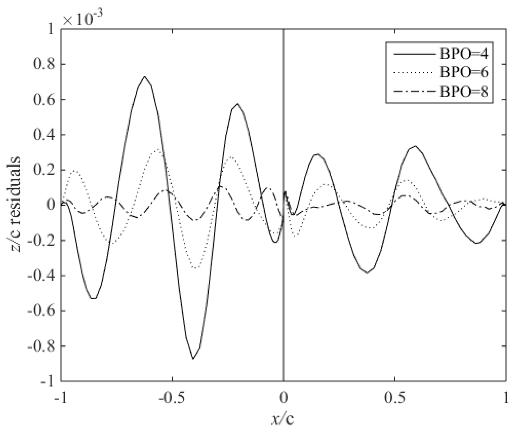
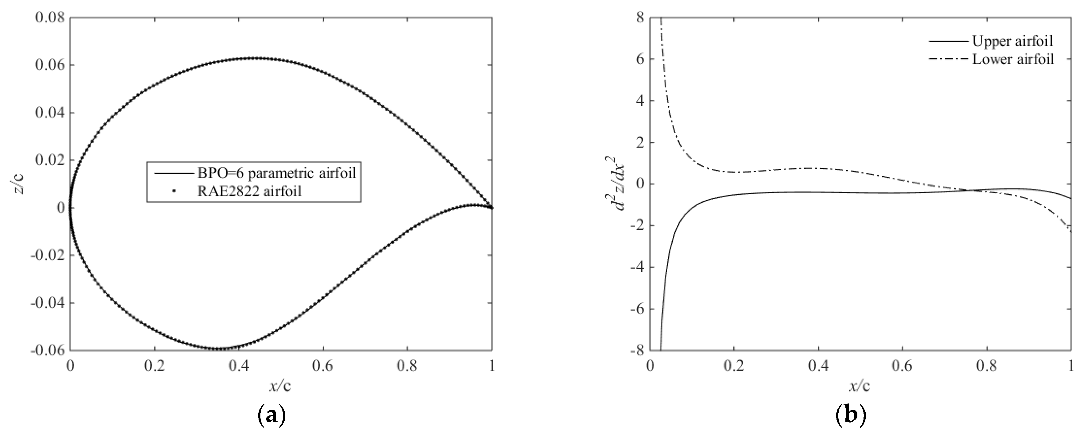
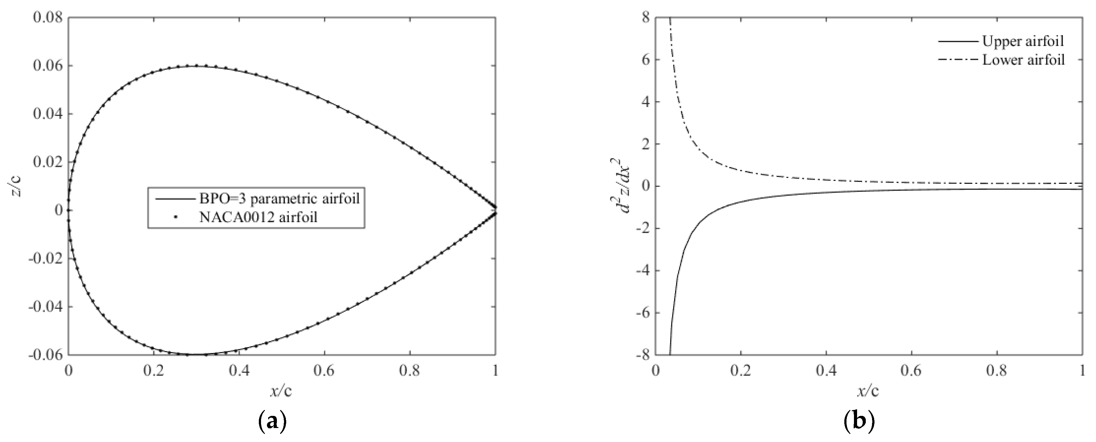
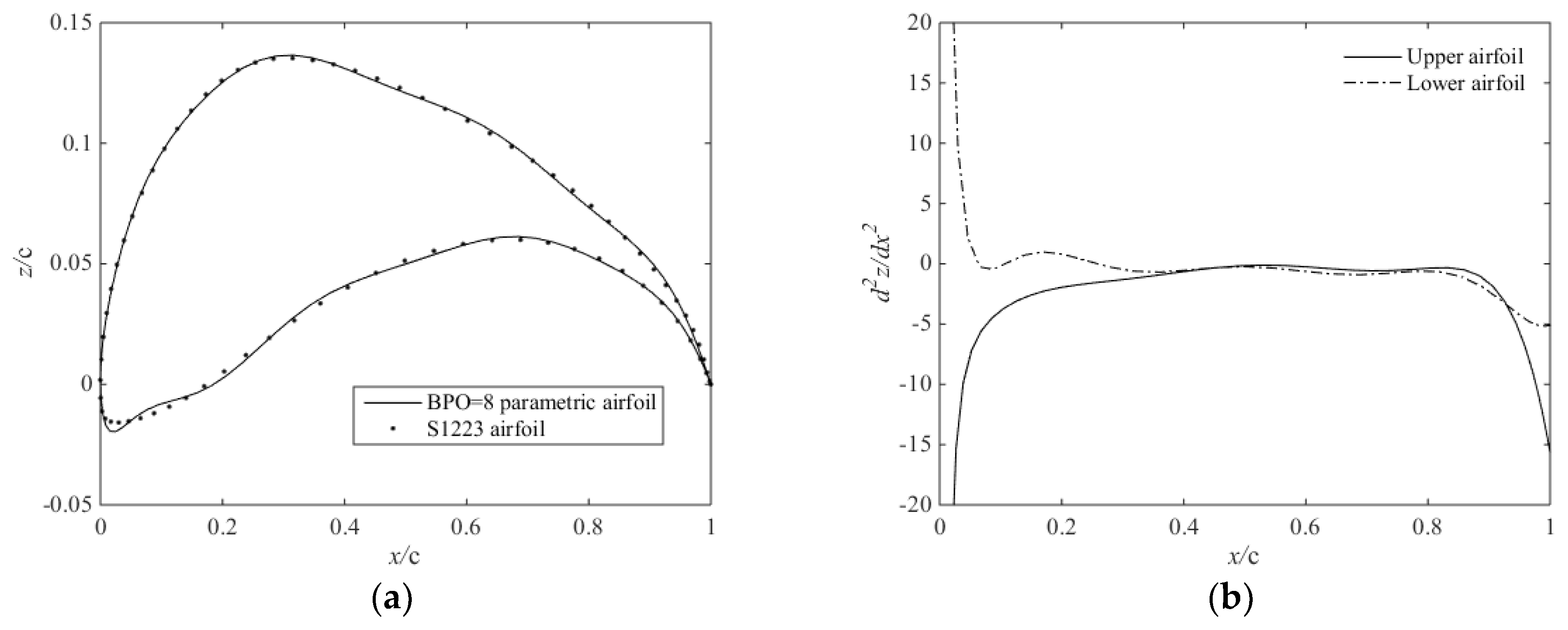
2.1. Airfoil Parameterization Based on the PEWI Method

The CST method, proposed by Kulfan [16,17,18], is widely used in the airfoil optimization. The universal parameterization for the complex aircraft components is developed by using this CST method, which is not limited only to the airfoils. For the normal airfoil with a rounded leading edge and pointed trailing edge, the difficulties in representing it mathematically are due to the infinite slope and second derivative requirement at the leading edge and large variations of curvature over the shape. The CST method can overcome these limits and represent the different types of geometries in a generic way. The general mathematical expression of the two-dimensional airfoil is as follows

$$\frac{z}{c}=\sqrt{\frac{x}{c}}\times (1-\frac{x}{c})\times {\displaystyle \sum _{i=0}^N[A_i\times {(\frac{x}{c})}^i]+\frac{x}{c}\times \frac{\Delta z_{te}}{c}}$$

(1)

This form can be rewritten as

$$\zeta (\psi )=C(\psi )S(\psi )+\psi {\zeta }_T$$

(2)

where $\psi =x/c$, $\xi =z/c$, ${\xi }_T=\Delta z_{te}/c$, $C(\psi )$ is the class function and $S(\psi )$ is the shape function

$$C(\psi )={(\psi )}^a{(1-\psi )}^b$$

(3)

$$S(\psi )=\frac{\xi (\psi )-\psi {\xi }_T}{\sqrt{\psi }(1-\psi )}={\displaystyle \sum _{i=0}^n{A}_i{\psi }_i}$$

(4)

The class parameters a and b for the general airfoil with a rounded leading edge and pointed trailing edge are set to 0.5 and 1.0. The Bernstein polynomial is employed as the shape function to describe the detailed shape as

$$B{P}_{i,n}(\psi )=K_i{\psi }^i{(1-\psi )}^{n-i}$$

(5)

where $K_i$ is the binomial coefficient and n is the order of Bernstein polynomial. The shape function is

$$S(\psi )={\displaystyle \sum _{i=0}^n{A}_{i}B{P}_{i,n}(\psi )}$$

(6)

The first weight coefficient of the Bernstein polynomial A₀ is directly related to the airfoil leading edge radius by the relation:

$$S(0)=A_0=\sqrt{\frac{2R_{le}}{c}}$$

(7)

The last weight coefficient of the Bernstein polynomial A_n is directly related to the airfoil boattail angle and trailing edge thickness by the relation:

$$S(1)=A_n=\tan (\theta )+\frac{\Delta z_{te}}{c}$$

(8)

Therefore, A₀ and A_n are two intuitive parameters of the CST method. The other coefficients of the CST method are nonintuitive. Equation (2) can be written as follows:

$$C(\psi ){\displaystyle \sum _{i=0}^n{A}_i\times \frac{n!}{i!\left(n-i\right)!}}\times {\psi }^i\times {(1-\psi )}^{n-i}=\zeta (\psi )-\psi {\zeta }_T$$

(9)

$$S_0(\psi )=C(\psi )\times \frac{n!}{i!\left(n-i\right)!}\times {\psi }^i\times {(1-\psi )}^{n-i}$$

(10)

To solve for the Bernstein coefficients $A_i$ to represent a given airfoil, Equation (9) can be built as follows:

$$\left(\begin{array}{cccc}{S}_0({\psi }_0)& S_1({\psi }_0)& \cdots & S_n({\psi }_0)\\ S_0({\psi }_1)& S_1({\psi }_1)& \cdots & S_n({\psi }_1)\\ ⋮& & \ddots & ⋮\\ S_0({\psi }_n)& S_1({\psi }_n)& & S_n({\psi }_n)\end{array}\right)\cdot \left(\begin{array}{c}{A}_0\\ A_1\\ ⋮\\ A_n\end{array}\right)=\left(\begin{array}{c}\zeta ({\psi }_0)-{\psi }_0{\zeta }_T\\ \zeta ({\psi }_1)-{\psi }_1{\zeta }_T\\ ⋮\\ \zeta ({\psi }_n)-{\psi }_n{\zeta }_T\end{array}\right)$$

(11)

$\mathit{S}=\left(\begin{array}{cccc}{S}_0({\psi }_0)& S_1({\psi }_0)& \cdots & S_n({\psi }_0)\\ S_0({\psi }_1)& S_1({\psi }_1)& \cdots & S_n({\psi }_1)\\ ⋮& & \ddots & ⋮\\ S_0({\psi }_n)& S_1({\psi }_n)& & S_n({\psi }_n)\end{array}\right)$ $\mathit{A}=\left(\begin{array}{c}{A}_0\\ A_1\\ ⋮\\ A_n\end{array}\right)$ $\mathit{Z}=\left(\begin{array}{c}\zeta ({\psi }_0)-{\psi }_0{\zeta }_T\\ \zeta ({\psi }_1)-{\psi }_1{\zeta }_T\\ ⋮\\ \zeta ({\psi }_n)-{\psi }_n{\zeta }_T\end{array}\right)$ where the linear equation is given by:

$$\mathit{SA}=\mathit{Z}$$

(12)

This is an ill-conditioned linear equation. If S or Z matrix had a slight fluctuation, such as δS or δZ, A might appear obvious errors. The condition number of S matrix can be used to weigh multiple of error. When the coefficient matrix S is obviously ill-conditioned, the condition number of S matrix is much larger than 1.

The PEWI method [14,15] is used to improve the condition number of S.

$$\mathit{S}+\alpha \mathit{E}$$

(13)

where S is the (n + 1)th order positive matrix, E is the (n + 1)th order unit matrix and α is the weight coefficient.

When α > 0, the condition number of $(\mathit{S}+\alpha \mathit{E})$ is proved smaller than S. It is very important to choose the appropriate α value. If α is too small, $(\mathit{S}+\alpha \mathit{E})$ matrix is still ill-conditioned and A matrix calculated by Equation (11) is inaccurate. And if α is too large, the convergence rate of the linear equation is very slow and the solution might be distorted. Therefore, we need choose the suitable α.

Taking Equation (13) into (12), this equation can be obtained.

$$(\mathit{S}+\alpha \mathit{E})\mathit{A}=\mathit{Z}+\alpha \mathit{A}$$

(14)

Bernstein coefficient matrix A can be calculated by the iterative algorithms. The iterative formula is as follows:

$$(\mathit{S}+\alpha \mathit{E}){\mathit{A}}^{(i+1)}=\mathit{Z}+\alpha {\mathit{A}}^{(i)}$$

(15)

where ${\mathit{A}}^{(i+1)}={\mathit{A}}^{(i)}+{\mathit{e}}^{(i)}$, so

$$\begin{array}{l}(\mathit{S}+\alpha \mathit{E})({\mathit{A}}^{(i)}+{\mathit{e}}^{(i)})=\mathit{Z}+\alpha {\mathit{A}}^{(i)}\Rightarrow \\ (\mathit{S}+\alpha \mathit{E}){\mathit{A}}^{(i)}+(\mathit{S}+\alpha \mathit{E}){\mathit{e}}^{(i)}=\mathit{Z}+\alpha {\mathit{A}}^{(i)}\Rightarrow \\ (\mathit{S}+\alpha \mathit{E}){\mathit{e}}^{(i)}=\mathit{Z}-{\mathrm{SA}}^{(i)}\end{array}$$

(16)

Obviously, we can gain the optimal solution of Equation (16) as long as 2-norm of ${\mathit{e}}^{(i)}$ reaches the setting precision. The iterative process is presented in Figure 1. i is the number of iterations of 2-norm and j is the number of iterations of the PEWI method. ε₁ and ε₂ are the setting errors. Δ is the step size of every iteration.

2.2. Fitting Airfoil by the CST Method

Three typical airfoils RAE2822, NACA0012, and S1223 are chosen in this study. These airfoils are fitted by the CST method. The fitting residuals are represented in Figure 2 and Figure 3. As the order of Bernstein polynomial increases, the residuals of RAE2822 and NACA0012 airfoil decrease. When the Bernstein polynomial is below 8th order, the root mean square error (RMSE) of RAE2822 and NACA0012 airfoil can meet the requirement of the typical wind-tunnel model tolerance. When BPO is 8, the RMSE of the RAE2822 airfoil can reach 2.2224 × 10⁻⁵ m. When BPO is 3, the RMSE of the NACA0012 airfoil can reach 7.7413 × 10⁻⁵ m.

The comparison between the CST parametric airfoil and the original RAE2822 airfoil is represented in Figure 4a. When the 6th order Bernstein polynomial is applied in the CST method, the fitting airfoil curve has in good agreement with the initial RAE2822 airfoil. When BPO = 6, the RAE2822 airfoil second derivatives are shown in Figure 4b. The upper and lower airfoils have no obvious fluctuations for BPO = 6. The NACA0012 airfoil has a finite thickness at the trailing edge. When BPO is 3, the fitting airfoil of CST method is closer to the initial NACA0012 airfoil in Figure 5a. When BPO = 3, the NACA0012 airfoil second derivatives are shown in Figure 5b. The upper and lower airfoils have no fluctuations for BPO = 3.

On the basis of the above analysis, we can conclude that low order Bernstein polynomial can accurately fit the small camber airfoil, such as RAE2822. And the RMSE can reach the requirement of typical wind-tunnel model tolerances.

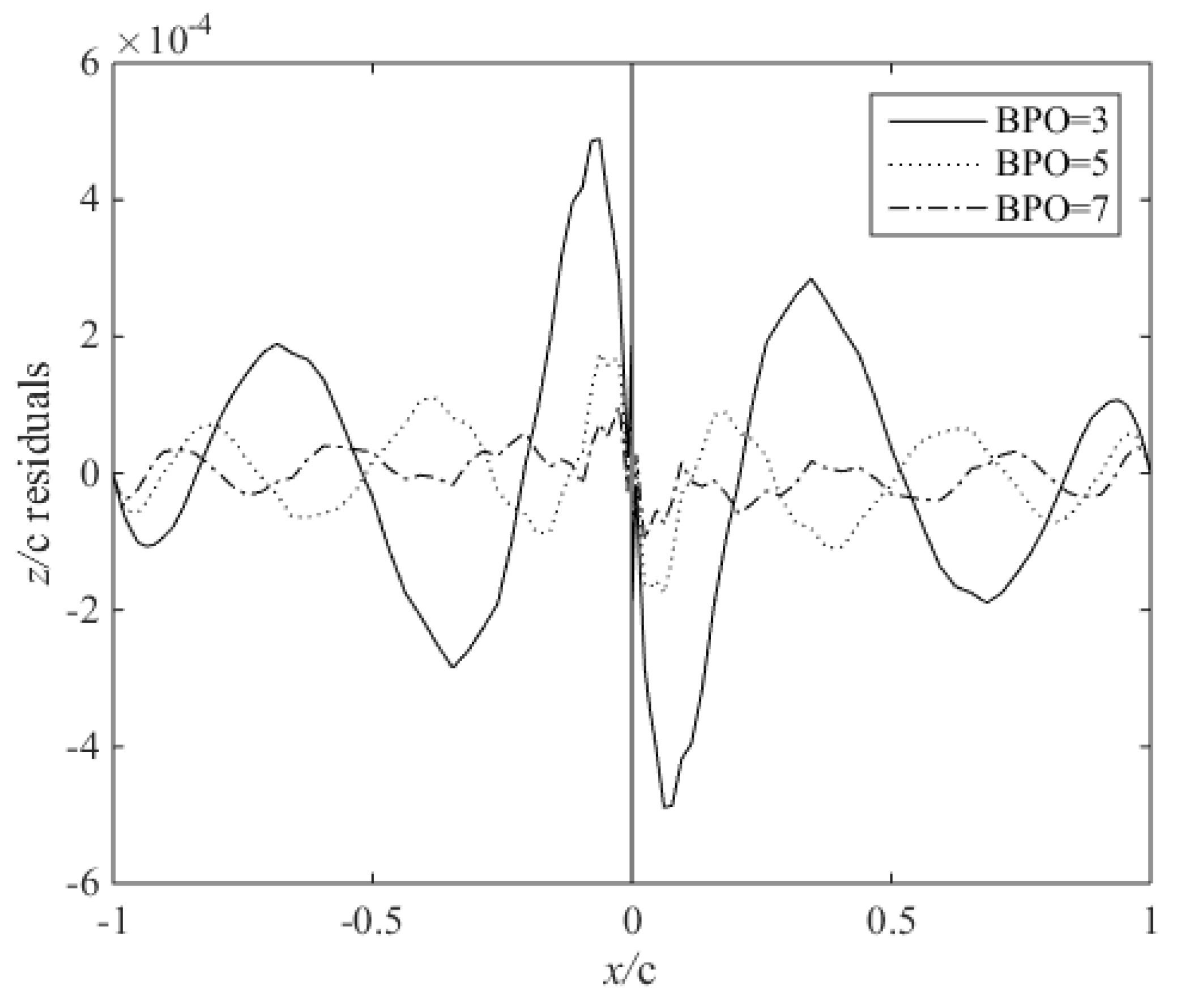
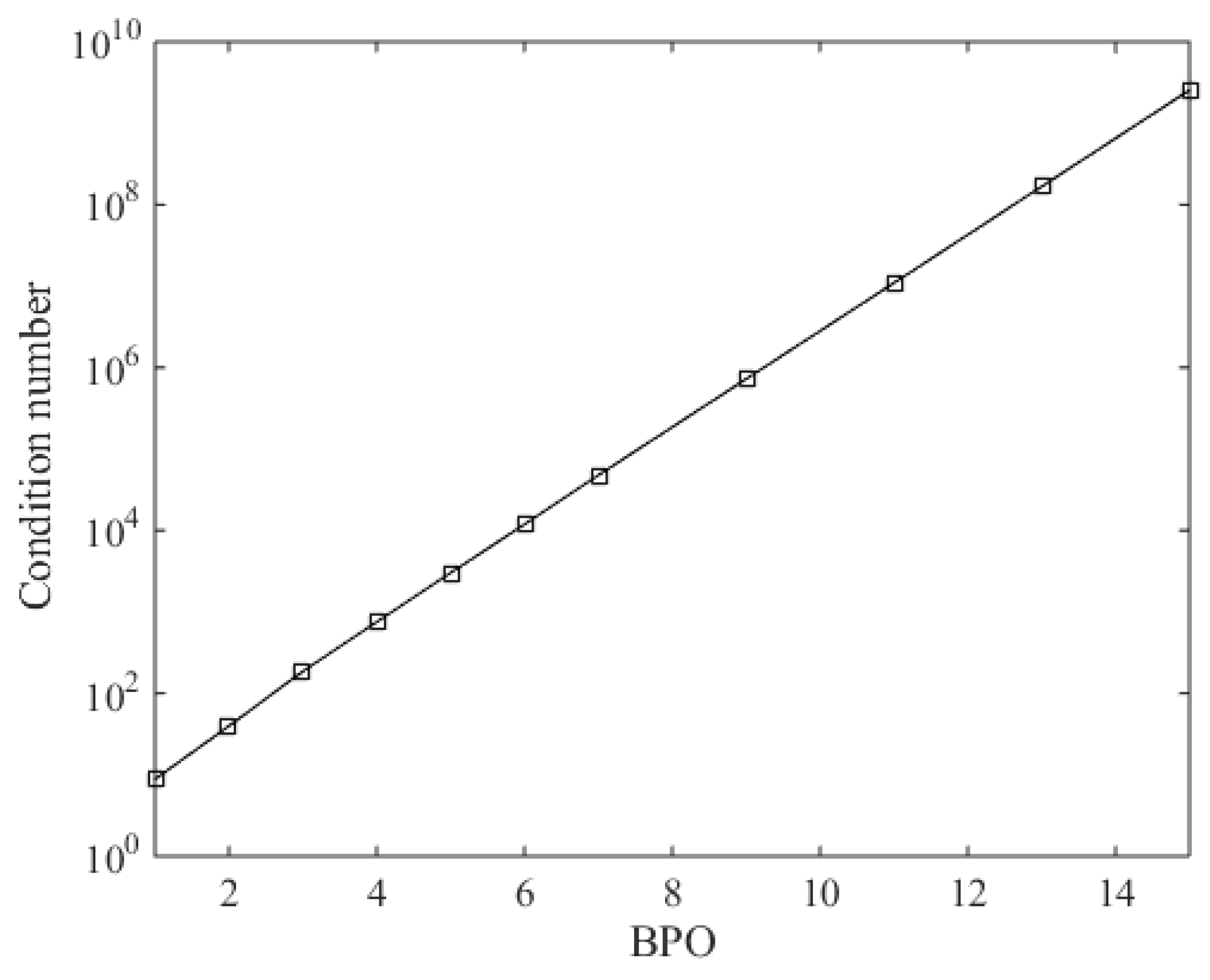
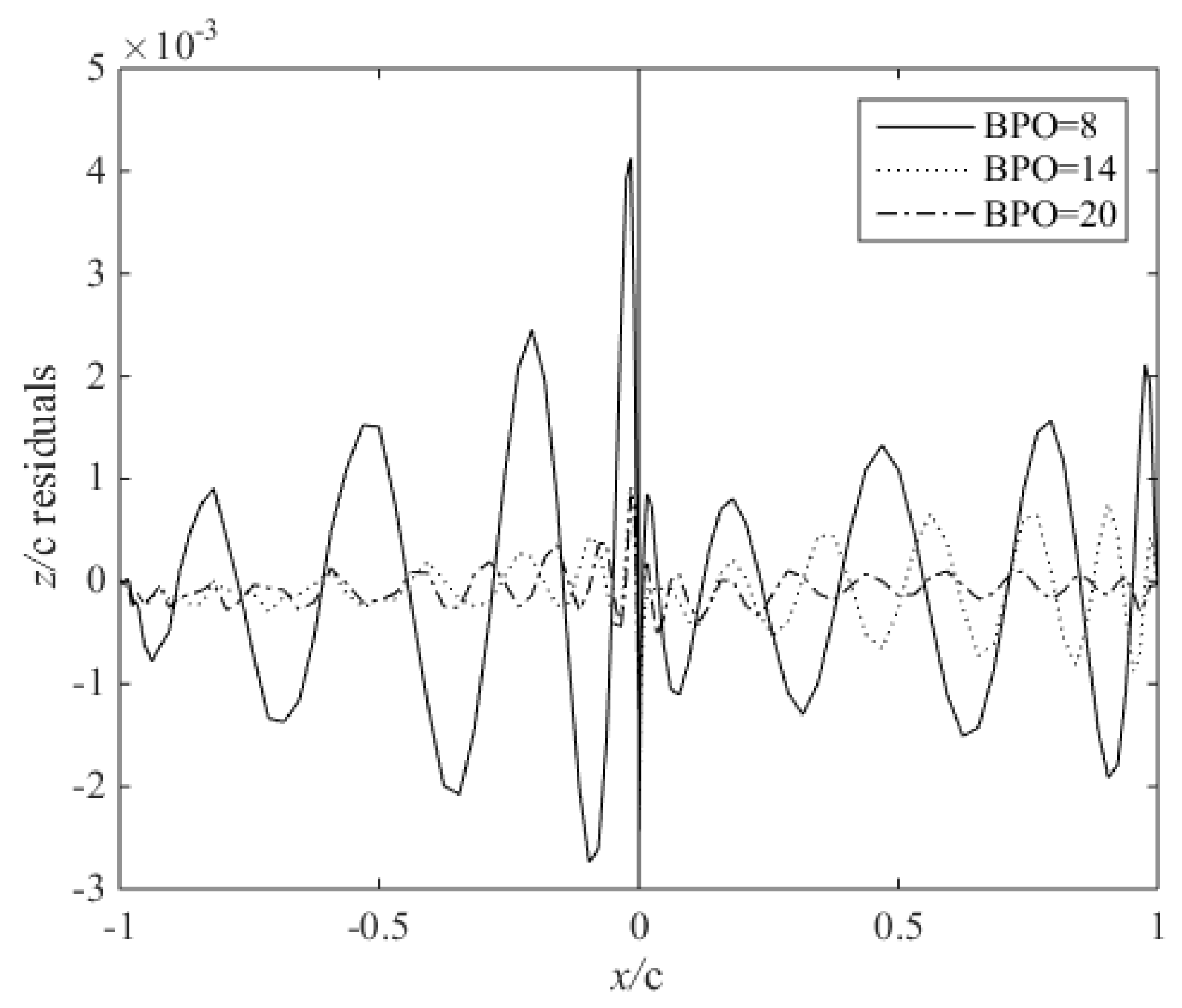
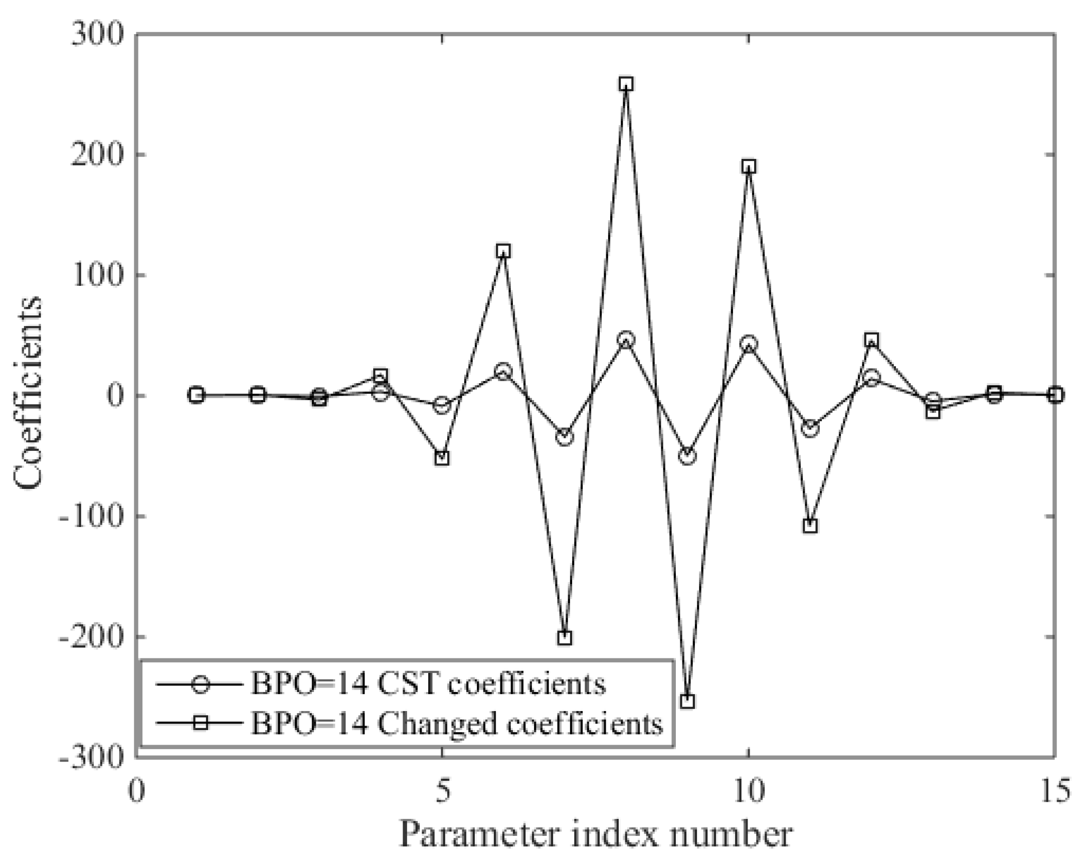
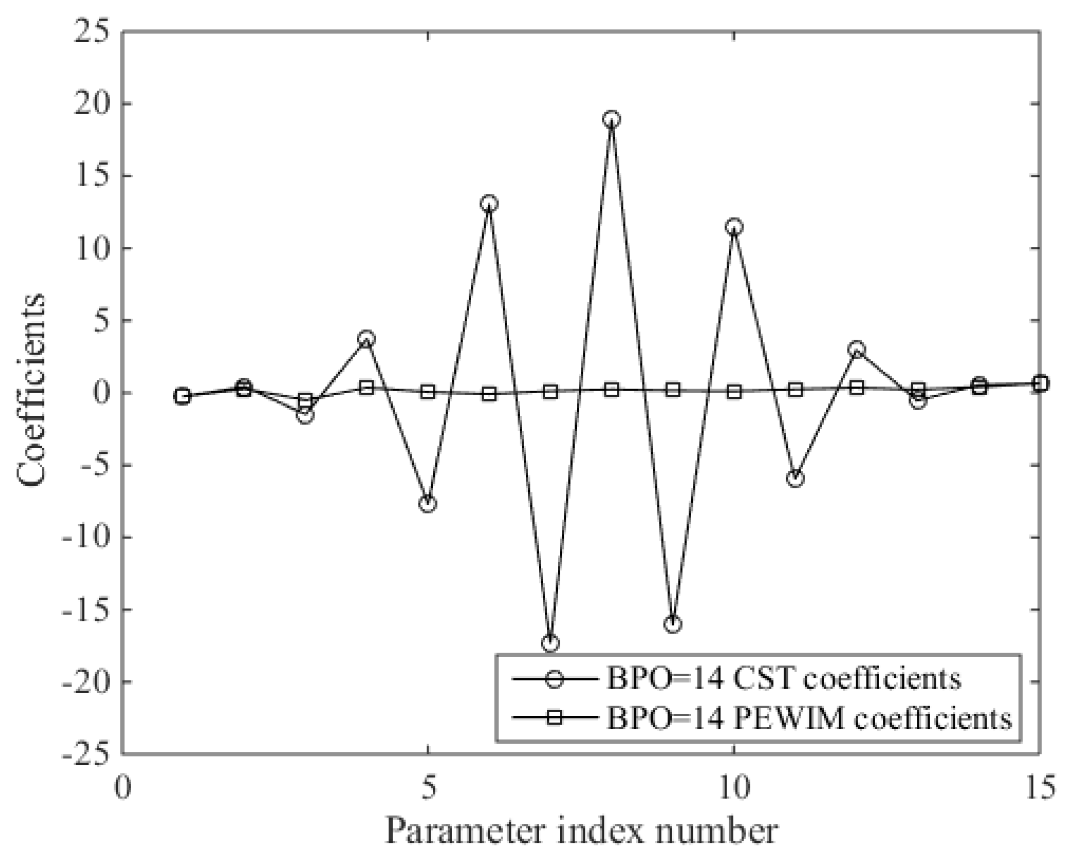
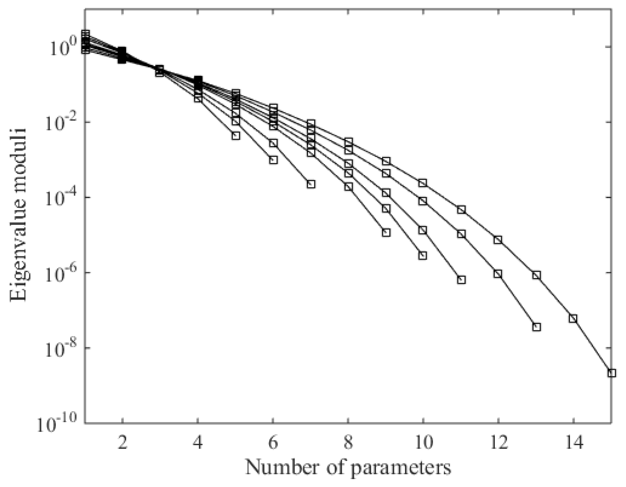
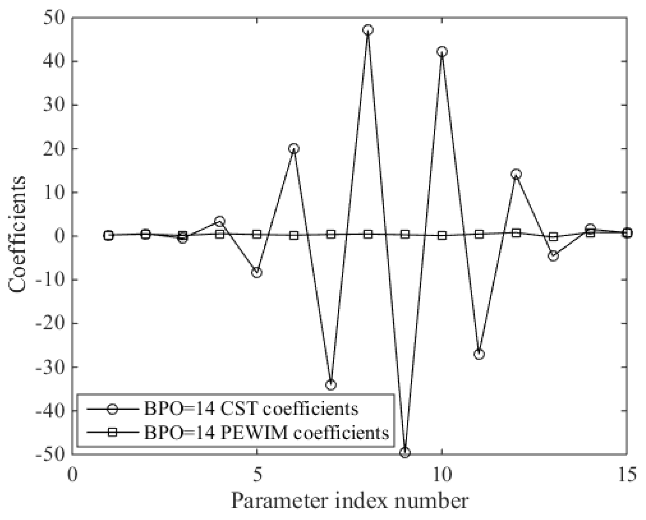
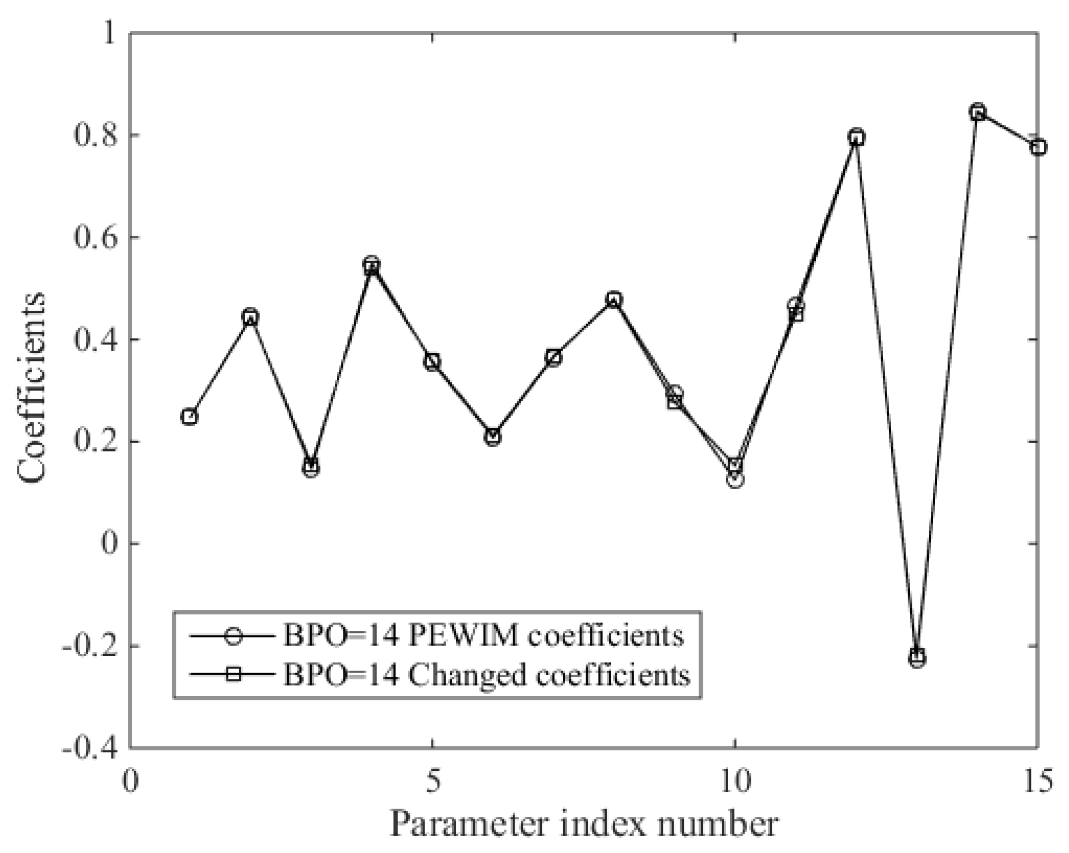
2.3. Parameter Matrix Analysis of the CST Method

The CST method is used to analyze the parameterization matrix of RAE2822 airfoil. As the order of Bernstein polynomial increases, the condition number of the parameterization matrix rapidly increases in Figure 6. The distribution of eigenvalue moduli of the parameterization matrix is presented in Figure 7. When the numbers of parameters change from 1 to 15, maximum eigenvalue has no obvious change. But minimum eigenvalue quickly approaches 0. So the parameterization matrix is close to extraordinary. The larger the condition number of the parameterization matrix is, the closer the parameterization matrix is to morbidity. The slight fluctuations of control point coordinates or the parameterization matrix can lead to the huge change of the solution vectors and vice versa. Therefore, two completely different solution vectors may generate quite close geometry and the difference between them may be less than the size of one grid cell.

CST method is selected to fit the high altitude laminar S1223 airfoil. Due to the large camber of S1223, the fitting airfoil has obvious deformation, especially the location of leading and trailing edge in Figure 8a. When BPO = 8, the S1223 airfoil second derivatives are shown in Figure 8b. The upper and lower airfoils have the obvious fluctuations. So it is necessary to increase the order of Bernstein polynomial. As mentioned above: the larger the order of the parameterization matrix is, the closer the parameterization matrix is to morbidity. And the slight fluctuations of the parameterization matrix or control point coordinates can lead to the large change of the solution vectors, which may go against the global optimum design of the airfoil. At the same time the more the parameters are, the lower the optimization efficiency is. Therefore, it is necessary to weigh the order of Bernstein polynomial and time consumed by the airfoil optimization.

The fitting residuals with different order Bernstein polynomial are presented in Figure 9. As the order of the polynomial parameterization increases, the residuals of S1223 airfoil decrease. So PEWI method is used to improve the coefficient matrix of the CST method. When BPO is 14, the RMSE can reach the requirement of typical wind-tunnel model tolerances. Meanwhile the variables are too many in BPO = 20. Hence, BPO = 14 is chosen.

When BPO is 14, the condition number of the coefficient matrix from the parameterization of the upper airfoil is 1.5819 × 10⁸ and the lower airfoil is 2.1266 × 10⁸. The coefficient matrix is obviously morbid. Any two elements of Z matrix change a little, such as: z₃ = z₃ + 0.00001, z₁₀ = z₁₀ + 0.00001, the element value of the parameterization matrix is shown in Figure 10. The amplitudes of the parameterization matrix have the huge changes. So it is disadvantageous for the optimization design of S1223 airfoil.

Aiming at the above problem, PEWI method is used to change the condition number of the coefficient matrix. When ε₁ and ε₂ are set as 0.000001 in Figure 1, α = 100 of the upper airfoil and α = 50 of the lower airfoil can be obtained. So the condition number of the upper airfoil change to 1.0154 and the lower is 1.0284. The Bernstein coefficients of the original CST method and the modified CST with PEWI method are showed in Figure 11 and Figure 12. The RMSE of the upper airfoil for the CST without PEWI is 4.4638 × 10⁻⁴ and the RMSE of the lower airfoil is 7.0917 × 10⁻⁴. And the RMSE of the upper airfoil for the CST with PEMI is 5.5753 × 10⁻⁴ and the RMSE of the lower airfoil is 7.3029 × 10⁻⁴. The fitting precision of the CST with PEWI is a little larger than the CST without PEWI. The essence of the CST method is to solve the linear equation by the least square method. The least square method is the unbiased estimate to obtain the minimum variance. Moreover, the PEWI method is a biased estimate which sacrifices the fitting precision to obtain the more stable linear equation and accurate solution. Because the linear equation is more stable, the fitting precision can be improved by increasing the order of the Bernstein polynomial.

When BPO is 14, coefficient matrix of S1223 airfoil is analyzed. Any two elements of Z matrix change small, such as: z₃ = z₃ + 0.00001, z₁₀ = z₁₀ + 0.00001, the element value of the parameterization matrix is shown in Figure 13. The parameterization matrix slightly changes, when using the modified CST with PEWI method. Therefore it is favorable for the optimization design of S1223 airfoil.

3. Aerodynamic Optimization Design of Airfoil

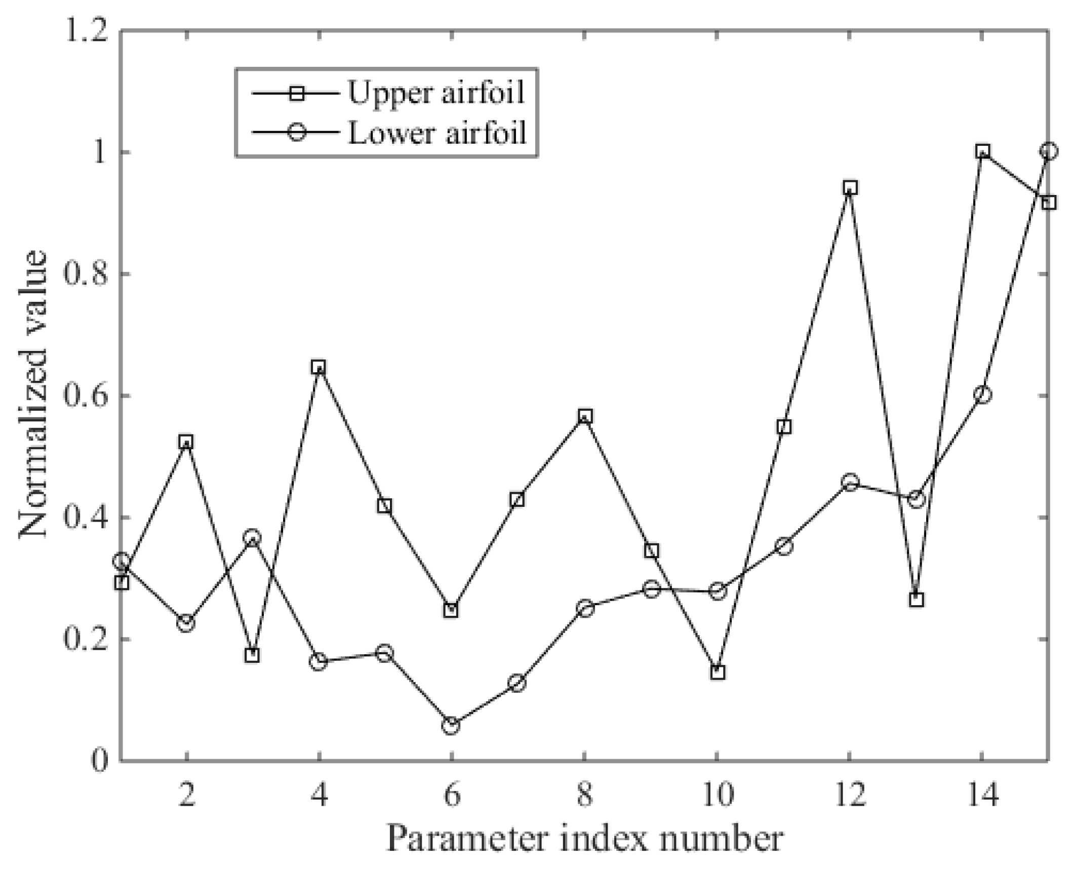
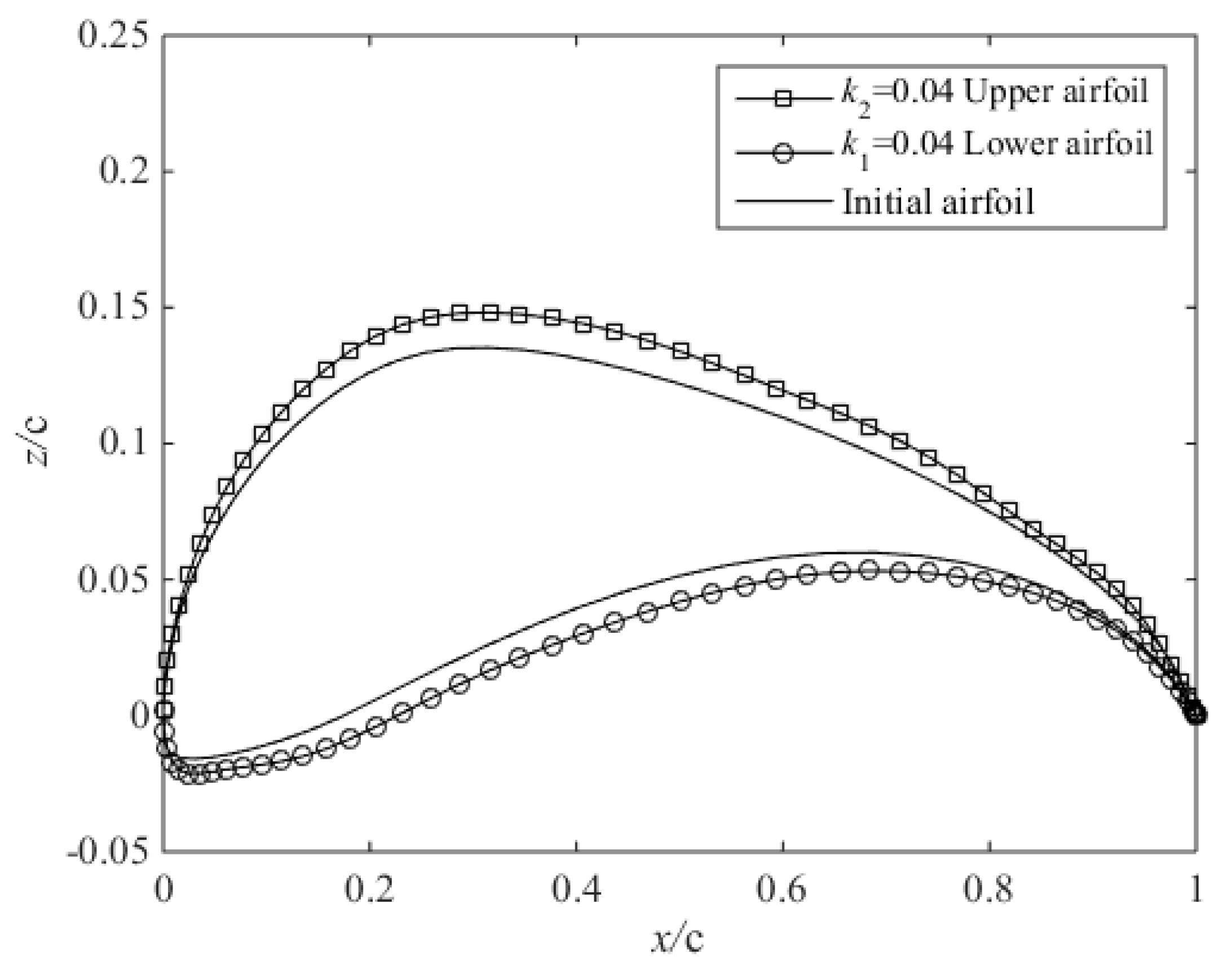
3.1. Normalization of the Design Parameters

S1223 is chosen as the aerodynamic optimum airfoil. 30 control parameters are used for the upper and lower airfoil. The keyword of optimization is to set up the scope of the parameter matrix. Normalization of the design parameters is proposed in the paper.

Parameter matrix is

$$\mathit{X}=\{x_1,x_2,\cdots ,x_n\}$$

(17)

The maximum absolute value of parameter matrix element is

$$x_{\max }=\max \left\{\right|x_1|,|x_2|,\cdots ,|x_n\left|\right\}$$

(18)

So the matrix of absolute value is

$${\mathit{X}}_1=\{\left|x_1\right|,\left|x_2\right|,\cdots ,\left|x_n\right|\}$$

(19)

Multiple matrix is

$${\mathit{X}}_2=\{\frac{x_{\max }}{\left|x_1\right|},\frac{x_{\max }}{\left|x_2\right|},1,\cdots ,\frac{x_{\max }}{\left|x_n\right|}\}$$

(20)

The value of ith element in ${\mathit{X}}_2$ is 1. Multiple matrix is used as the criterion to enlarge and shrink the other elements. The range of the criterion is [−k₁, k₂]. And k₁, k₂ > 0. So the range of every element in ${\mathit{X}}_2$ is

$$\begin{array}{l}{x}_1\in [x_1(1-k_1\frac{x_{\max }}{\left|x_1\right|}),x_1(1+k_2\frac{x_{\max }}{\left|x_1\right|})]\\ x_2\in [x_2(1-k_1\frac{x_{\max }}{\left|x_2\right|}),x_2(1+k_2\frac{x_{\max }}{\left|x_2\right|})]\\ \begin{array}{ccc}\begin{array}{cc}\begin{array}{cc}& \end{array}& \end{array}& & \end{array}⋮\\ \begin{array}{ccc}\begin{array}{cc}\begin{array}{cc}& \end{array}& \end{array}& & \end{array}⋮\\ x_i\in [x_i(1-k_1),x_2(1+k_2)]\\ \begin{array}{ccc}\begin{array}{cc}\begin{array}{cc}& \end{array}& \end{array}& & \end{array}⋮\\ \begin{array}{ccc}\begin{array}{cc}\begin{array}{cc}& \end{array}& \end{array}& & \end{array}⋮\\ x_n\in [x_n(1-k_1\frac{x_{\max }}{\left|x_n\right|}),x_n(1+k_2\frac{x_{\max }}{\left|x_n\right|})]\end{array}$$

(21)

Parameter matrix values of normalization are represented in Figure 14. Assuming that k₁ and k₂ are the value of upper and lower airfoil. The boundary change of S1223 can be obtained, when k_2upper is 0.04, k_1lower is 0.04 and k_1upper is 0.04, k_2lower is 0.04. Figure 15 and Figure 16 show that the leading edge and trailing edge of S1223 have the obvious changes which expand the species of S1223 airfoil.

3.2. Design of Experiment

The approximation model is established by the sample data and the design of experiment (DOE) method is adopted to sample the design space. DOE methods include the orthogonal arrays (OA) [19], the full factorial design (FFD), the latin hypercube design (LHD) [20] and the optimal Latin hypercube design (Opt LHD) [21]. By comparison with the LHD, the experiment data of the Opt LHD are uniformly distributed in the design space. And the Opt LHD has good space filling and equilibration ability [22]. So the Opt LHD is selected to obtain the sample data.

3.3. Radial Basis Functions Neural Network Model

The Kriging [23], RSM [24], and RBF [25] methods are widely used in the surrogate model. The disadvantage of the Kriging is that model construction can be very time-consuming and complex [26]. The RSM is not suitable to create a global metamodel for a highly nonlinear response [27]. The RBF is suitable for the highly nonlinear problems and these problems can be modelled with limited number of samples [27]. And when BPO is 14, the least samples of the quadratic RSM and the Kriging with the quadratic regression model are 496. It is a huge computation for the airfoil optimization.

The neural network consists of three layers: the input layer, the hidden layer and the output layer, which has the ability to approximate the complex nonlinear function. So the RBF neural network model [5] is used to establish the approximation model of the airfoil aerodynamic data.

Firstly, the RBF neural network is trained by the sample data of DOE. The approximation relationship between aerodynamic coefficients and design parameters can be obtained. Secondly, it is necessary to evaluate the prediction precision, in order to ensure the adaptability of the approximation model. There are two indicators to assess the precision of the approximation model and they are the root mean square error (RMSE) and correlation coefficient (R²). The closer the RMSE is to 0, the higher the precision of the approximation model is. Generally, the range of R² is from 0 to 1. The closer R² is to 1, the better the fitting precision is. The value of R² is larger than 0.9 [28]. In this paper, the thresholds of the RMSE and R² are set as 0.03 and 0.98. The number of initial sample data is 100 and 50 random samples are used to analyze the errors of the approximation model. If the RMSE and R² cannot reach the requirements of thresholds, 100 new samples are added into the initial samples until the RMSE and R² satisfy the setting values. When the number of the samples is increase to 300, the RMSE and R² of the lift coefficients are 0.00485 and 0.99955. And the RMSE and R² of the drag coefficients are 0.03 and 0.98619.

In the paper the experimental data of the Opt LHD are 300 samples for the S1223 airfoil. The approximation model based on the RBF neural network is established to calculate aerodynamic coefficients of the S1223 airfoil. 50 samples are used to analyze the errors of the approximation model.

3.4. Genetic Algorithms

Genetic algorithms are search-optimization methods which use principles of natural genetics and natural selection. In such methods, the possible solutions for a certain problem are represented by some form of biological population, which evolves over generations to adapt to an environment by selection, crossover, and mutation. Instead of working with a single solution at each iteration of the process, a genetic algorithm (GA) works with a number of solutions, known as a population [2]. The traditional GA only has one population. The multi-island genetic algorithm (MIGA) has several sub-populations. Then the selection, crossover, and mutation operations are executed for the every sub-population like the traditional GA. And the individuals of the sub-populations are exchanged by the migration operation. The calculation speed of MIGA can be faster than those of traditional genetic algorithms [29]. The MIGA parameters of S1223 airfoil optimization are presented in

Table 1. Parameters of MIGA.

Parameters	Value
Number of generations	25
Number of sub-populations	10
Number of individuals on each sub-population	20
Interval generations of migration	4
Crossover rate	0.9
Mutation rate	0.01
Migration rate	0.3

.

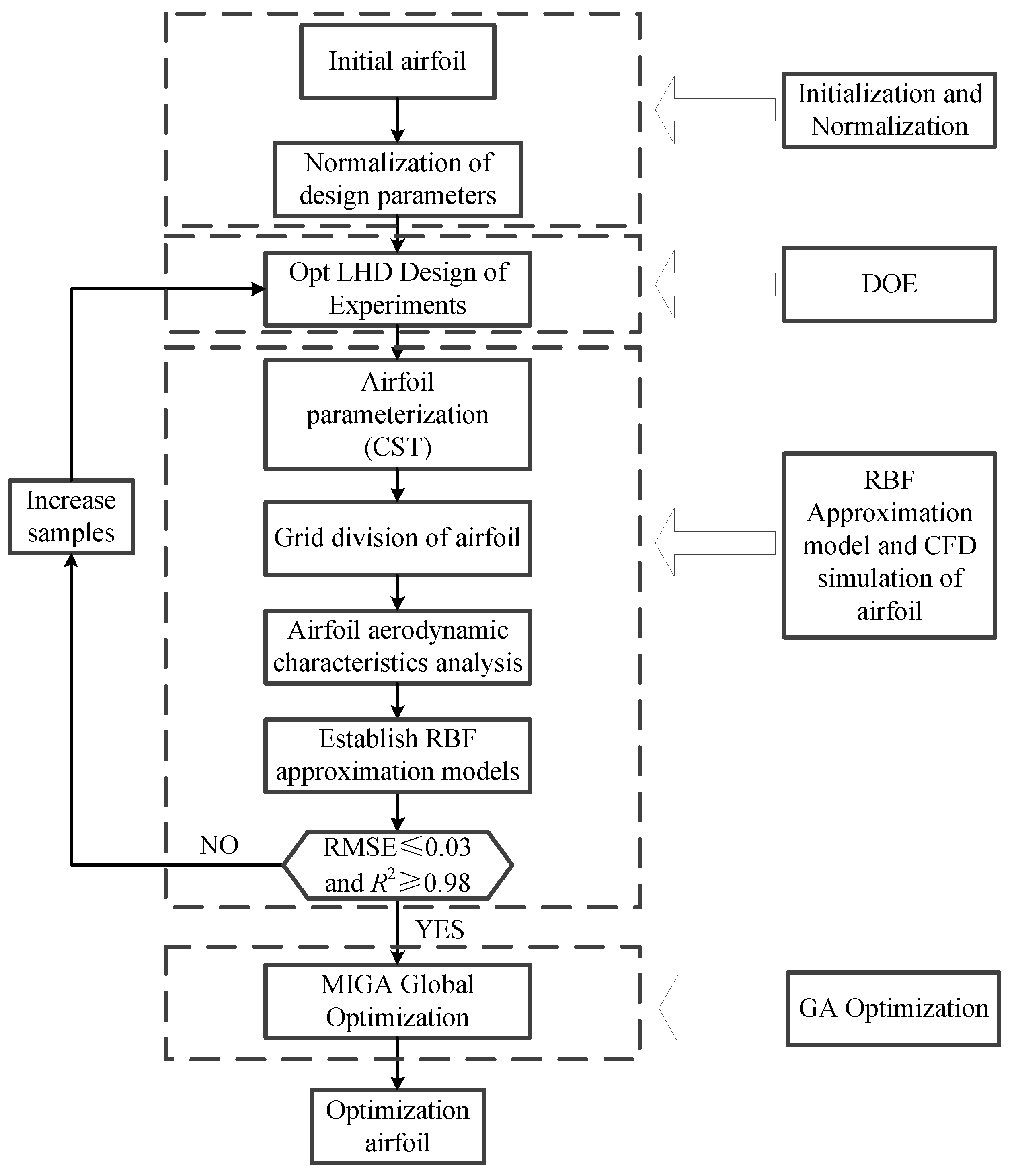
3.5. Optimization Process

The design process is represented in Figure 17. It is divided into 4 parts, namely initialization and normalization of the design parameters, DOE, RBF approximation model and CFD simulation of airfoil, and GA optimization.

As we all know, the stratosphere low speed aircrafts include the stratosphere airship and long-endurance solar unmanned aerial vehicle. At the height of 20 km, the air density is 0.088 kg/m³, the viscosity is 1.4216 × 10⁻⁵ kg/(m·s). The speed of these aircrafts ranges from 20 m/s to 80 m/s and the range of Reynolds number fall between 10⁵ and 10⁶. The S1223 airfoil is the laminar and high lift airfoil, which has the good aerodynamic performance under the condition of the low Reynolds number [30,31]. So it can be used in the design of the high altitude propeller and the solar wing. The aerodynamic characteristics of the S1223 airfoil are analyzed in this paper. The optimization goal is to raise the lift–drag ratio of S1223. The aerodynamic constraints are the lift coefficient and drag coefficient. The geometric constraint is the area of the S1223 airfoil. The design conditions are that Ma = 0.1, α = 4°, Re = 1.86 × 10⁵. The objective function is

$$\begin{array}{l}\max \begin{array}{cc}& K=C_L/C_D\end{array}\\ s.t.\begin{array}{cc}& \end{array}Ma=0.1\begin{array}{cc}& Re\end{array}=1.86\times {10}^5\begin{array}{cc}& \alpha =4^{\circ }\end{array}\\ \begin{array}{cccc}& & & \end{array}{C}_L\ge 0.95C_{L0}\\ \begin{array}{cccc}& & & \end{array}{C}_D\le C_{D0}\\ \begin{array}{cccc}& & & \end{array}S\ge 0.95S_0\end{array}$$

where $C_{L0}$ is the lift coefficient of the intial airfoil, $C_{D0}$ is the drag coefficient of the intial airfoil, K is the lift-drag ratio and $S_0$ is the initial area.

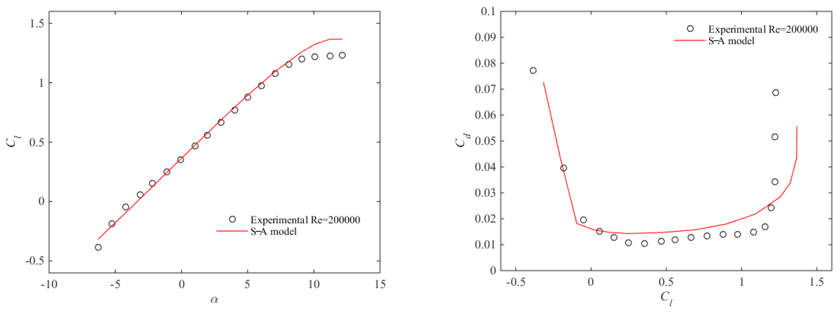
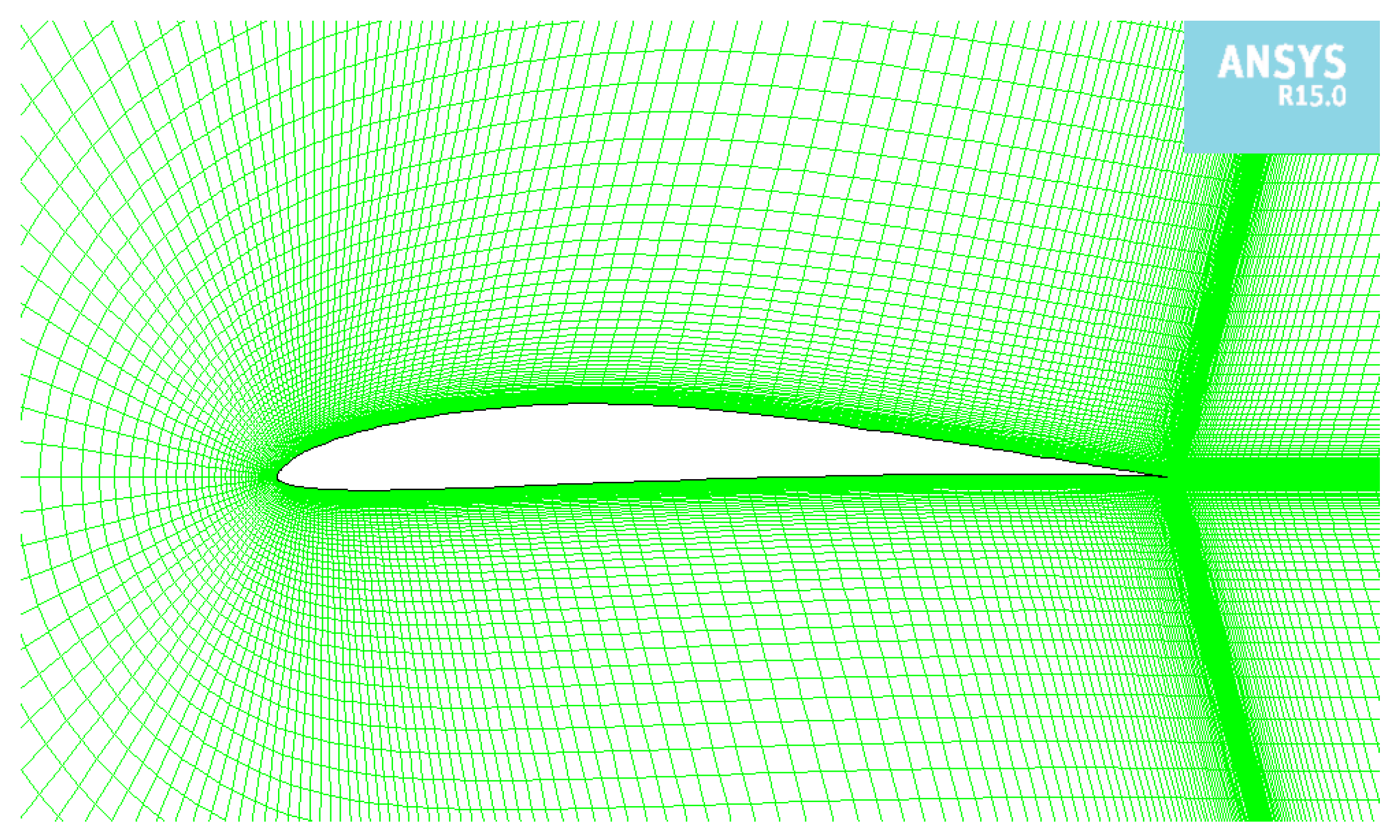
3.6. Validation of CFD Model

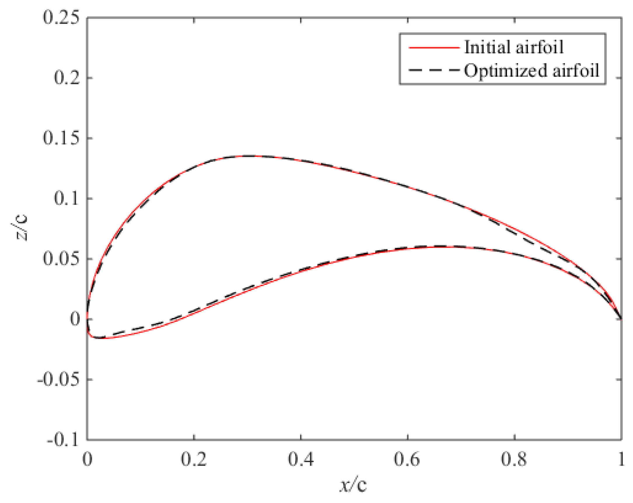
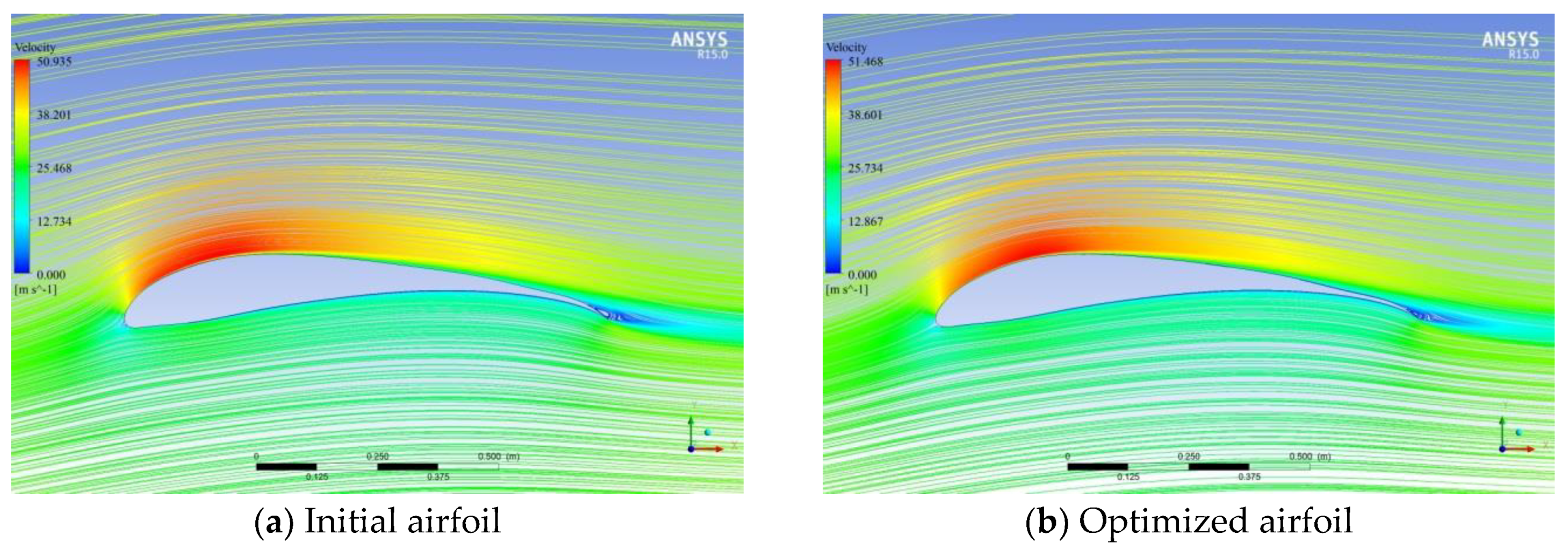
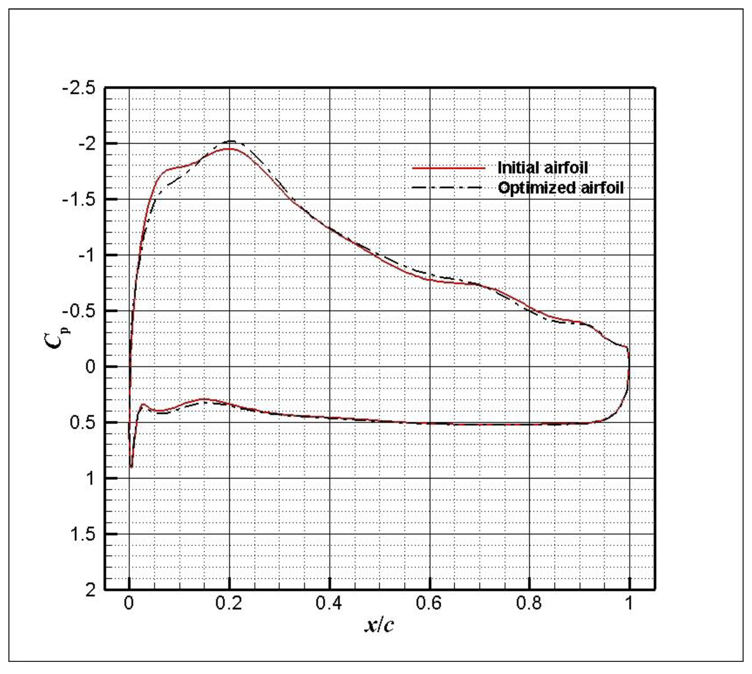
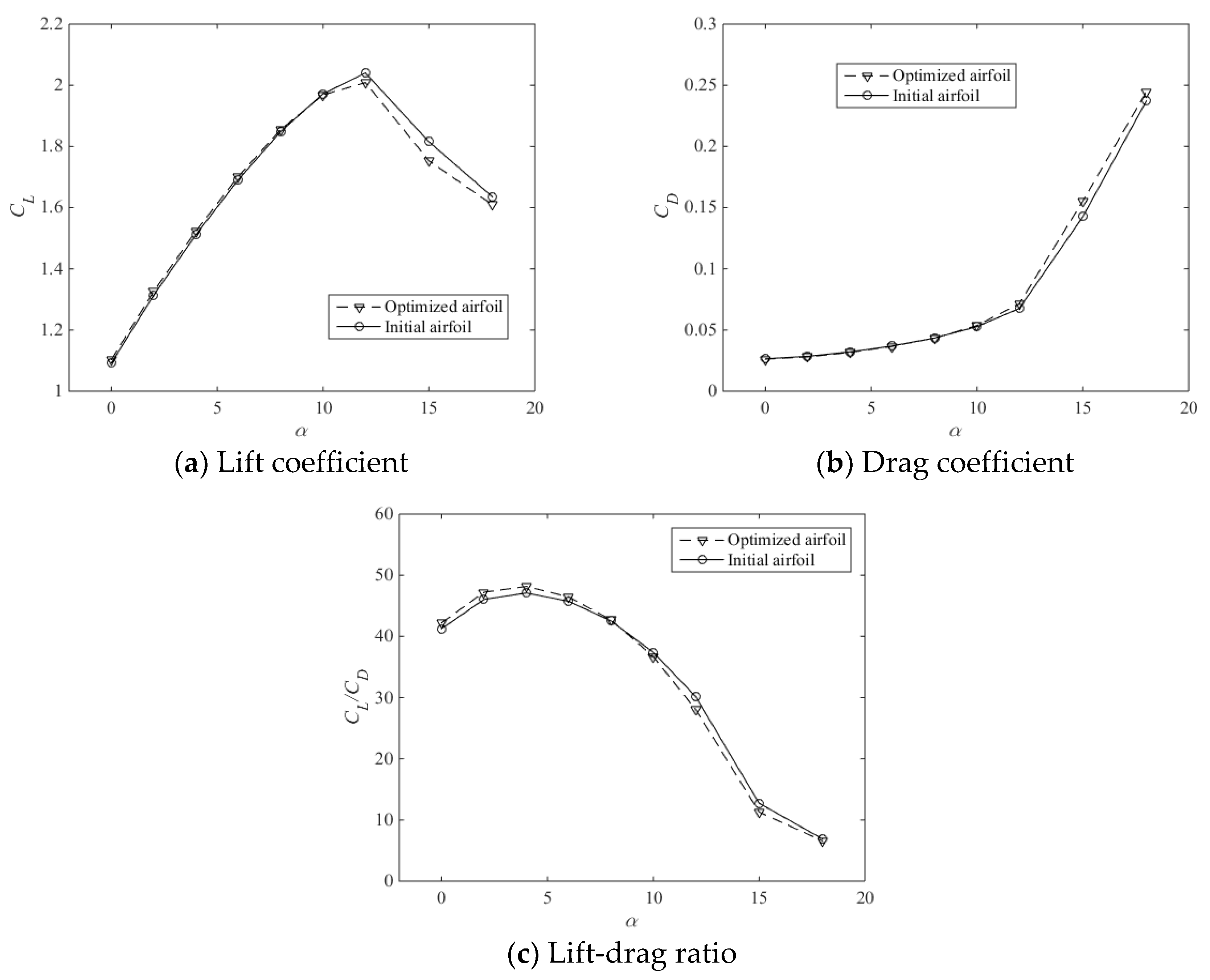
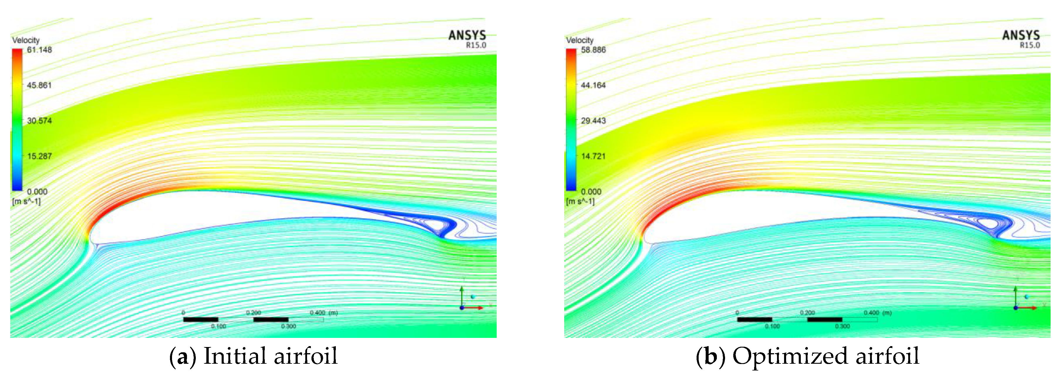
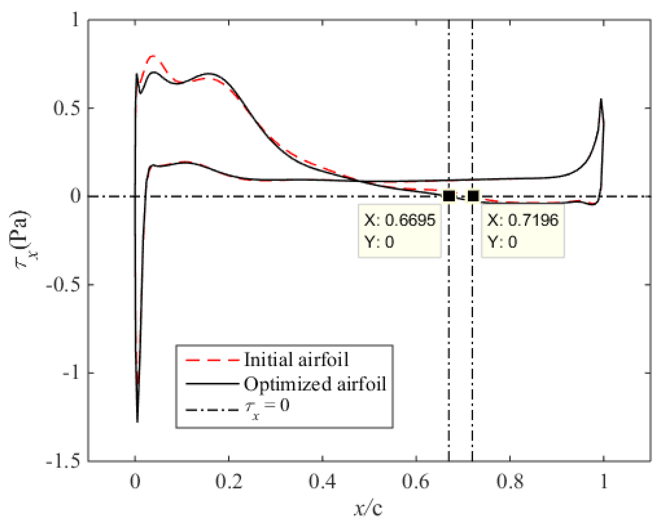
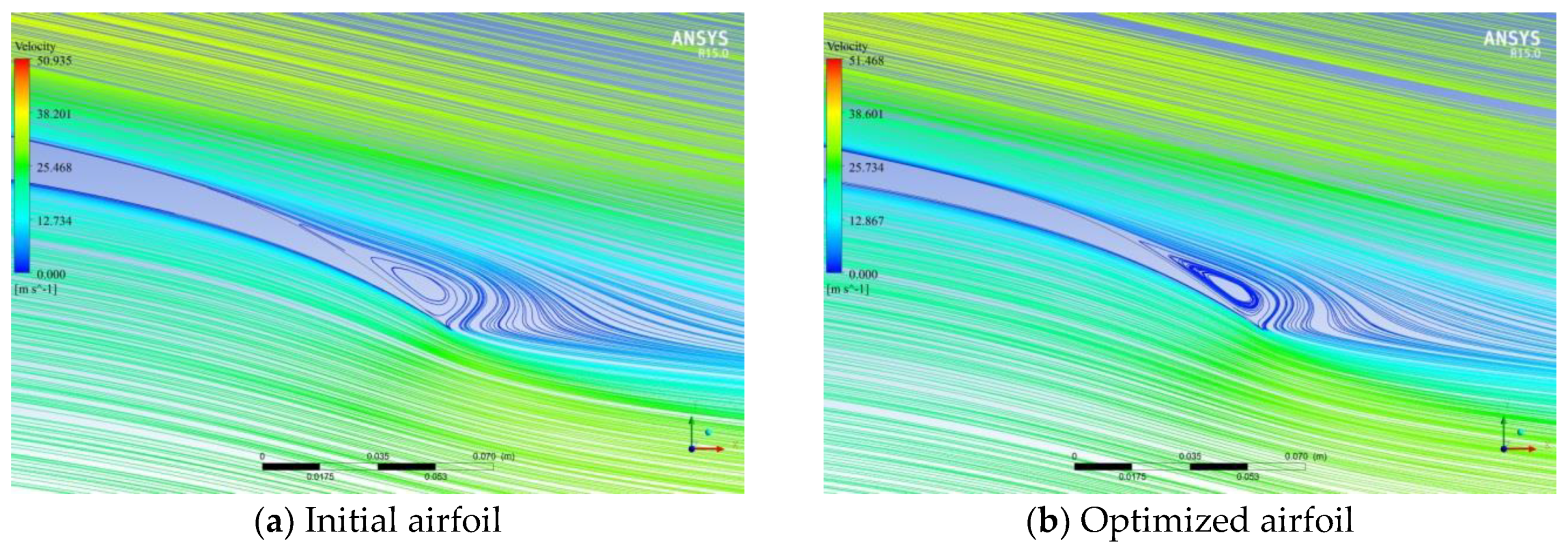
The numerical simulations are validated by considering the experiment data of the low-speed and low-Reynolds number E387 airfoil [31]. C-type structure grids are generated by the Gambit software in Figure 18. The number of grids is 500 × 100. The first layer mesh height is set as 1.08 × 10⁻⁴ m which can ensure y plus is close to 1. Aerodynamic coefficients of the E387 airfoil are obtained by the Fluent software. The governing equations are Reynolds-Averaged Navier–Stokes equations. The boundary condition is the pressure far field. The turbulence model is the Spalart–Allmaras model. The S–A model is the single equation turbulence model which is widely used in the airfoil aerodynamic simulation. The simulation conditions are: Re = 2 × 10⁵, μ = 1.7894 × 10⁻⁵ kg/(m·s), ρ = 1.225 kg/m³.

The airfoil performance predicted for Re = 2 × 10⁵ by S-A turbulence model is compared to the University of Illinois Urbana-Campaign (UIUC) [31] wind-tunnel measurements in Figure 19. The results show that the CFD simulations are in good agreement with the experiments. So the CFD model is feasible and accurate.

4. Results

There are 15 design variables of the upper airfoil. The range of them is from −0.0339 to +0.0339. The lower airfoil also has 15 design variables whose range is from −0.0263 to +0.0263. 300 different-shaped airfoil samples are generated by the Opt LHD. The lift and drag coefficients of every sample airfoil are calculated by the numerical simulation using the SA model. These aerodynamic data are trained as the samples of the RBF approximation model. Moreover the errors of RBF are analyzed using 50 additional Opt LHD samples. The results are listed in

Table 2. Evaluation of the approximation model.

Aerodynamic Coefficient	RMSE	R2
CL	0.00485	0.99955
CD	0.03	0.98619

.

The initial and optimized airfoils are shown in Figure 20. The leading edge radius of S1223 airfoil decreases and the camber of the whole airfoil increases. It leads to the increase of the lift coefficient and decrease of the drag coefficient. Optimization results are represented in

Table 3. Optimization results.

Upper Airfoil Variables	Min	Max	Optimum	Lower Airfoil Variables	Min	Max	Optimum
Aup1	−0.0339	0.0339	−0.02188	Alow1	−0.0263	0.0263	0.01346
Aup2	−0.0339	0.0339	−0.0246	Alow2	−0.0263	0.0263	0.00836
Aup3	−0.0339	0.0339	0.01508	Alow3	−0.0263	0.0263	0.00994
Aup4	−0.0339	0.0339	−0.00465	Alow4	−0.0263	0.0263	0.02331
Aup5	−0.0339	0.0339	0.0144	Alow5	−0.0263	0.0263	−0.01926
Aup6	−0.0339	0.0339	−0.01463	Alow6	−0.0263	0.0263	0.0073
Aup7	−0.0339	0.0339	0.01213	Alow7	−0.0263	0.0263	0.00906
Aup8	−0.0339	0.0339	−0.03027	Alow8	−0.0263	0.0263	0.02173
Aup9	−0.0339	0.0339	0.02574	Alow9	−0.0263	0.0263	−0.02401
Aup10	−0.0339	0.0339	0.02347	Alow10	−0.0263	0.0263	0.01487
Aup11	−0.0339	0.0339	−0.00374	Alow11	−0.0263	0.0263	9.00×10−5
Aup12	−0.0339	0.0339	−0.02438	Alow12	−0.0263	0.0263	−0.0015
Aup13	−0.0339	0.0339	−0.02732	Alow13	−0.0263	0.0263	0.00396
Aup14	−0.0339	0.0339	−0.03367	Alow14	−0.0263	0.0263	9.70×10−4
Aup15	−0.0339	0.0339	−0.02324	Alow15	−0.0263	0.0263	0.00871

.

Aerodynamic characteristics of the optimized airfoil are compared with the initial airfoil under the condition of Ma = 0.1 and Re = 1.86 × 10⁵. The results are shown in Figure 21.

It can be seen from Figure 21 that the lift coefficient of optimized airfoil maximumly increases by about 1%, the drag coefficient maximumly decreases by about 1.57% and the lift-drag ratio maximumly increases by about 2.57% when angle of attack changes from 0° to 8°. When angle of attack is greater than 8°, the lift coefficient of the optimized airfoil reduces and drag coefficient increases. Because the leading edge radius of the optimized airfoil decreases and the trailing edge thickness becomes thin, compared with the initial airfoil. Therefore, it leads to the expansion of the laminar flow separation area for the optimized airfoil.

Velocity streamlines of the optimized and initial airfoils under the condition of 12° are presented in Figure 22. It indicates that the laminar flow area of the initial airfoil is larger than the optimized airfoil.

In the case of 12°, the wall shear stresses in x axis direction of the initial and optimized airfoil are shown in Figure 23. τ_x of the initial airfoil is less than 0 in the location of 0.7196 chord. So the coordinate of the laminar flow separation point is 0.7196 chord of the initial S1223 airfoil. And τ_x of the optimized airfoil is less than 0 in the location of 0.6695 chord. It indicates that the coordinate of the laminar flow separation point is 0.6695c for the optimized airfoil. Therefore, the laminar flow separation area of the optimized airfoil is bigger than the initial airfoil. And the lift coefficient of the optimized airfoil reduces and drag coefficient increases at the large angle of attack compared with the initial S1223 airfoil.

The optimum results that lift-drag ratio increases by 2.27% and the drag coefficient decreases by 1.4% are listed in

Table 4. Aerodynamic performances of the initial and optimized airfoils.

	CL	CD	CL/CD	ΔCL	ΔCD	ΔCL/CD
Initial airfoil	1.5119	0.0321	47.1
Optimized airfoil (RBF)	1.5247	0.03165	48.17	0.85%	−1.40%	2.27%
CFD	1.5244	0.03165	48.16	0.83%	−1.40%	2.25%

. The aerodynamic data of the RBF model obtained by GA optimization are similar with CFD simulation.

The velocity streamlines of the optimized and initial airfoils under the condition of 4° are presented in Figure 24 and Figure 25. Pressure coefficient distribution of the initial and optimized airfoil is represented in Figure 26. It is obvious that the optimized airfoil has the larger laminar zone than the initial airfoil. In Figure 25 the reverse flow zone of the initial airfoil is bigger. So the drag of the optimized airfoil is smaller than the initial airfoil. And the optimized airfoil has the larger velocity than the initial airfoil at the upper airfoil. So the dynamic pressure of the optimized airfoil is bigger and the lift is larger than the initial airfoil. From Figure 26, though the pressure of the upper airfoil increases near the trailing edge for the optimized airfoil, the pressure of the upper airfoil from 15% to 70% chord decreases. And the pressure of the lower airfoil from 5% to 90% chord increases. So the lift of the optimized airfoil is larger than the initial airfoil.

5. Conclusions

The CST method is widely used in the airfoil parameterization for the airfoil aerodynamic design. The low order Bernstein polynomial, which can reach the requirement of the fitting precision, can be applied to fit the symmetric NACA0012 airfoil and small camber RAE2822 airfoil. But the low order Bernstein polynomial cannot reach the fitting precision for the large camber S1223 airfoil. So the number of control parameters needs to be added. The more the number of control parameters is, the closer the coefficient matrix of CST is to morbidity. Therefore, the PEWI method is proposed to improve the ill-conditioned matrix and this method is suitable for the optimization design of airfoil. And the robustness of the CST method can be enhanced.

Setting the range of design parameters is the crucial step for the airfoil optimization. So the normalization method of design variables is put forward in this paper and it is helpful for the airfoil optimization to obtain the suitable design parameters.

The samples of aerodynamic coefficients for the S1223 airfoil are generated by the optimal Latin hypercube design method. The RBF neural network is trained by these samples. The S1223 airfoil is optimized to obtain the maximum lift-drag ratio by GA. The optimum airfoil has the higher camber by comparison with the initial airfoil. The optimum results in which the lift-drag ratio increases by 2.27% and the drag coefficient decreases by 1.4% are good values for the airfoil design.

References

1. Zhu, F.; Qin, N. Intuitive Class/Shape Function Parameterization for Airfoils. AIAA J. 2013, 52, 17–25. [Google Scholar] [CrossRef]
2. Antunes, A.P.; Azevedo, J.L.F. Studies in Aerodynamic Optimization Based on Genetic Algorithms. J. Aircr. 2014, 51, 1002–1012. [Google Scholar] [CrossRef]
3. Liu, Y.X.; Yang, C.; Song, X.C. An airfoil parameterization method for the representation and optimization of wind turbine special airfoil. J. Therm. Sci. 2015, 24, 99–108. [Google Scholar] [CrossRef]
4. Wang, C.; Gao, Z.H.; Huang, J.T.; Zhao, K.; Li, J. Smoothing methods based on coordinate transformation in a linear space and application in airfoil aerodynamic design optimization. Sci. China Technol. Sci. 2015, 58, 297–306. [Google Scholar] [CrossRef]
5. Ariyarit, A.; Kanazaki, M. Multi-Objective Efficient Global Optimization Applied to Airfoil Design Problems. Appl. Sci. 2017, 7, 1318. [Google Scholar] [CrossRef]
6. Morris, C.C.; Allison, D.L.; Schetz, J.A.; Kapania, R.K.; Sultan, C. Parametric Geometry Model for Design Studies of Tailless Supersonic Aircraft. J. Aircr. 2014, 51, 1455–1466. [Google Scholar] [CrossRef]
7. Zhang, Y.F.; Fang, X.M.; Chen, H.X.; Fu, S.; Duan, Z.Y.; Zhang, Y.J. Supercritical natural laminar flow airfoil optimization for regional aircraft wing design. Aerosp. Sci. Technol. 2015, 43, 152–164. [Google Scholar] [CrossRef]
8. Vu, N.A.; Lee, J.W.; Shu, J.I. Aerodynamic design optimization of helicopter rotor blades including airfoil shape for hover performance. Chin. J. Aeronaut. 2013, 26, 1–8. [Google Scholar] [CrossRef]
9. Vu, N.A.; Lee, J.W. Aerodynamic design optimization of helicopter rotor blades including airfoil shape for forward flight. Aerosp. Sci. Technol. 2015, 42, 106–117. [Google Scholar] [CrossRef]
10. Ceze, M. A Study of the CST Parameterization Characteristics; Report No.: AIAA-2009-3767; AIAA: Reston, VA, USA, 2009. [Google Scholar]
11. Guan, X.H.; Li, Z.K.; Song, B.F. A study on CST aerodynamic shape parameterization method. Acta Aeronaut. Astronaut. Sin. 2012, 33, 625–633. (In Chinese) [Google Scholar]
12. Guan, X.H.; Song, B.F.; Li, Z.K. Comparison of the CSRT and the CST parameterization methods. Acta Aeronaut. Astronaut. Sin. 2014, 32, 228–234. (In Chinese) [Google Scholar]
13. Wang, X.; Cai, J.S.; Qu, K.; Liu, C.Z. Airfoil optimization based on improved CST parametric method and transition model. Acta Aeronaut. Astronaut. Sin. 2015, 36, 449–461. (In Chinese) [Google Scholar]
14. Wu, X.; Shao, R.; Zhu, Y. New iterative improvement of a solution for an Ill-conditioned system of linear equations based on a linear dynamic system. Comput. Math. Appl. 2002, 44, 1109–1116. [Google Scholar] [CrossRef]
15. Salkuyeh, D.K.; Fahim, A. A new iterative refinement of the solution of ill-conditioned linear system of equations. Int. J. Comput. Math. 2011, 88, 950–956. [Google Scholar] [CrossRef]
16. Kulfan, B.M.; Bussoletti, J.E. Fundamental parametric geometry representations for aircraft component shapes. In Proceedings of the 11th AIAA/ISSMO Multidisciplinary Analysis and Optimization Conference, Portsmouth, VA, USA, 6 September 2006. [Google Scholar]
17. Kulfan, B.M. Recent Extensions and Applications of the ‘‘CST” Universal Parametric Geometry Representation Method; Report No.: AIAA-2007-7709; AIAA: Reston, VA, USA, 2007. [Google Scholar]
18. Kulfan, B.M. New Supersonic Wing Far-Field Composite-Element Wave-Drag Optimization Method. J. Aircr. 2009, 46, 1740–1758. [Google Scholar] [CrossRef]
19. Owen, A.B. Orthogonal Arrays for Computer Experiments, Integration and Visualization. Stat. Sin. 1992, 2, 439–452. [Google Scholar]
20. McKay, M.D.; Beckman, R.J.; Conover, W.J. A Comparison of Three Methods for Selecting Values of Input Variables in the Analysis of Output from a Computer Code. Technometrics 1979, 21, 239–245. [Google Scholar]
21. Park, J.S. Optimal Latin-hypercube designs for computer experiments. J. Stat. Plan. Inference 1994, 39, 95–111. [Google Scholar] [CrossRef]
22. Lai, Y.Y. Parameters Optimization Theory of Isght and Explain of Examples; Beihang University Press: Beijing, China, 2012; pp. 88–102. (In Chinese) [Google Scholar]
23. Sacks, J.; Welch, W.J.; Mitchell, T.J.; Wynn, H.P. Design and analysis of computer experiments. Stat. Sci. 1989, 4, 409–423. [Google Scholar] [CrossRef]
24. Simpson, T.W.; Lin, D.K.; Chen, W. Sampling strategies for computer experiments: Design and analysis. Int. J. Reliabil. Appl. 2001, 2, 209–240. [Google Scholar]
25. Hardy, R.L. Multiquadratic equations of topography and other irregular surface. J. Geophys. Res. 1971, 76, 905–1915. [Google Scholar] [CrossRef]
26. Jin, R.; Chen, W.; Simpson, T.W. Comparative studies of metamodelling techniques under multiple modelling criteria. Struct. Multidiscip. Optim. 2001, 23, 1–13. [Google Scholar] [CrossRef]
27. Fang, H.; Horstemeyer, M.F. Global response approximation with radial basis functions. Eng. Optim. 2006, 38, 407–424. [Google Scholar] [CrossRef]
28. Zhou, C.; Wang, Z.J.; Zhi, J.Y. Aerodynamic optimization design of adaptive airfoil leading edge based on isight. J. Shanghai Jiaotong Univ. 2014, 48, 1122–1133. (In Chinese) [Google Scholar]
29. Zhao, D.J.; Wang, Y.K.; Cao, W.W.; Zhou, P. Optimization of suction control on an airfoil using multi-island genetic algorithm. Procedia Eng. 2015, 99, 696–702. [Google Scholar] [CrossRef]
30. Ma, R.; Zhong, B.; Liu, P. Optimization design study of low-Reynolds-number high-lift airfoils for the high-efficiency propeller of low-dynamic vehicles in stratosphere. Sci. China Technol. Sci. 2010, 53, 2792–2807. [Google Scholar] [CrossRef]
31. Selig, M.S.; Guglielmo, J.J. High-lift low Reynolds number airfoil design. J. Aircr. 1997, 34, 72–79. [Google Scholar] [CrossRef]
Figure 1. Iterative process of the pivot element weighting iterative method. RMSE: root mean square error; CST: class function/shape function transformation method.
Algorithms 11 00163 g001
Figure 2. CST parameterization residuals of the RAE2822 airfoil.
Algorithms 11 00163 g002
Figure 3. CST parameterization residuals of the NACA0012 airfoil.
Algorithms 11 00163 g003
Figure 4. (a) Comparison between the CST parametric airfoil and the RAE2822 airfoil (b) RAE2822 airfoil second derivatives when BPO = 6.
Algorithms 11 00163 g004
Figure 5. (a) Comparison between the CST parametric airfoil and the NACA0012 airfoil (b) NACA0012 airfoil second derivatives when BPO = 3.
Algorithms 11 00163 g005
Figure 6. Spectral condition number of the parameterization matrix. BPO: Bernstein polynomials.
Algorithms 11 00163 g006
Figure 7. Eigenvalue moduli of the parameterization matrix.
Algorithms 11 00163 g007
Figure 8. (a) Comparison between the CST parametric airfoil and the S1223 airfoil (b) S1223 airfoil second derivatives when BPO = 8.
Algorithms 11 00163 g008
Figure 9. CST parameterization residuals of the S1223 airfoil.
Algorithms 11 00163 g009
Figure 10. Comparison of the parameterization matrix using CST.
Algorithms 11 00163 g010
Figure 11. Comparison between the CST method and the PEWI method of the upper airfoil.
Algorithms 11 00163 g011
Figure 12. Comparison between the CST method and the PEWI method of the lower airfoil.
Algorithms 11 00163 g012
Figure 13. Comparison of parameterization matrix using the PEWI method.
Algorithms 11 00163 g013
Figure 14. Normalization of parameterization matrix values.
Algorithms 11 00163 g014
Figure 15. Range of the S1223 airfoil at k2upper = 0.04 and k1lower = 0.04.
Algorithms 11 00163 g015
Figure 16. Range of the S1223 airfoil at k1upper = 0.04 and k2lower = 0.04.
Algorithms 11 00163 g016
Figure 17. Optimization process of airfoil. LHD: Latin hypercube design; RBF: radial basis functions.
Algorithms 11 00163 g017
Figure 18. Grids around the E387 airfoil.
Algorithms 11 00163 g018
Figure 19. Lift and lift to drag polar curves of E387 airfoil at Re = 2 × 10⁵. S–A: Spalart–Allmaras model.
Algorithms 11 00163 g019
Figure 20. Comparison between initial and optimized airfoil.
Algorithms 11 00163 g020
Figure 21. Comparisons of aerodynamic characteristics between the optimized airfoil and the initial S1223 airfoil.
Algorithms 11 00163 g021
Figure 22. Velocity streamlines at the 12° angle of attack.
Algorithms 11 00163 g022
Figure 23. Wall shear stress of x axis direction.
Algorithms 11 00163 g023
Figure 24. Velocity streamlines of the initial and optimized airfoils at α = 4°.
Algorithms 11 00163 g024
Figure 25. Velocity streamlines of the initial and optimized airfoils near the trailing edge at α = 4°.
Algorithms 11 00163 g025
Figure 26. Pressure coefficient distribution of the initial and optimized airfoils.
Algorithms 11 00163 g026