Article

A Hybrid Algorithm for Optimal Wireless Sensor Network Deployment with the Minimum Number of Sensor Nodes

1
National School of Applied Sciences of Tetouan, Abdelmalek Essaâdi University, Tétouan 93000, Morocco
2
Department of Computer Science and Engineering School of Engineering-University of Cádiz, Cádiz 11001, Spain
*
Author to whom correspondence should be addressed.
Algorithms 2017, 10(3), 80; https://doi.org/10.3390/a10030080
Submission received: 15 June 2017 / Revised: 7 July 2017 / Accepted: 12 July 2017 / Published: 18 July 2017

Abstract

:
Wireless sensor network (WSN) applications are rapidly growing and are widely used in various disciplines. Deployment is one of the key issues to be solved in WSNs, since the sensor nodes’ positioning affects highly the system performance. An optimal WSN deployment should maximize the collection of the desired interest phenomena, guarantee the required coverage and connectivity, extend the network lifetime, and minimize the network cost in terms of energy consumption. Most of the research effort in this area aims to solve the deployment issue, without minimizing the network cost by reducing unnecessary working nodes in the network. In this paper, we propose a deployment approach based on the gradient method and the Simulated Annealing algorithm to solve the sensor deployment problem with the minimum number of sensor nodes. The proposed algorithm is able to heuristically optimize the number of sensors and their positions in order to achieve the desired application requirements.

1. Introduction

Nowadays, WSNs are employed in many applications designed for different purposes such as: environment and habitat monitoring [1,2], traffic control [3], health care application [4], home automation [5] etc. The main purpose of WSN applications is the event detection in a Region of Interest (RoI), where sensor nodes are deployed to monitor any ongoing events. Besides the sensing function, communication is another major function of a sensor network [6]. Generally, when sensor nodes are spread out, they start to sense the information and forward it to the sink node using multi-hop paths [7], then to the base station (BS), where intelligent decisions can be made. Figure 1 shows the network architecture of a WSN application dedicated to monitor an area.
WSN deployment is one of the major challenges of WSN research. It affects almost all its performance metrics, such as the connectivity between sensor nodes, the coverage, and the network’s lifetime. These factors are the essential criteria to evaluate a WSN’s performance in order to choose a WSN design from a number of candidates. Consequently, a considerable amount of research in the field of WSNs is dedicated to address the WSN deployment issue [8,9]. Generally, deployment can be deterministic, namely pre-determined, or non-deterministic [9]. The pre-determined deployment, where the locations of sensor nodes are specified, is usually used in a friendly environment and when nodes are expensive. When the environment is dangerous and inaccessible, e.g., the only way of deployment is using helicopters or automatic vehicles, as in this case, the deployment is non-deterministic or in other words random [9].
WSN applications can only operate for a given period of time or as long as possible, due to sensor nodes’ limited supply of energy from batteries. Hence, the network lifetime becomes a very important issue [10]. In the phase of deployment, if nodes are too close to each other, coverage overlapping and redundant nodes could occur, which generates unnecessary data transfer and more traffic load, and if the distance between nodes is too large, nodes will consume more energy to distribute data through the network. This constraint deeply affects the energy consumption of nodes. Consequently, it’s very important to determine the optimal distance between nodes. Hence, network designers should not only be concerned about the basic requirements, such as the network connectivity and coverage, but also try to improve the network lifetime and reduce the network cost [11].
The Simulated Annealing (SA) algorithm is a classical meta-heuristic global optimization method inspired by the annealing process of material in metallurgy and is widely used for global optimization problems. Several approaches were developed to improve coverage and connectivity using the SA algorithm [12,13,14,15]. In this article, we propose a hybrid algorithm based on the Gradient method and the SA algorithm to solve the WSN placement problem while defining the optimal number of nodes to deploy, to ensure the required coverage and connectivity in the case of a deterministic deployment, where all sensor nodes positions are well controlled. The main contributions of this paper are as follows:
  • A Hybrid algorithm based on the gradient and the SA algorithm is demonstrated for the sensor deployment problem, with the selection of the minimal number of nodes.
  • Simulation results are shown to prove the efficiency of the proposed technique.
  • A comparison with other approaches is concluded in order to evaluate the efficiency of the proposed algorithm.
This paper is organized as follows, in Section 2, we overview some basic concepts of WSN. In Section 3, the related works are discussed. Then in Section 4, we explain how the SA algorithm can optimize the deployment process. A problem description and formulation is presented in Section 5. Finally and before concluding, simulation results using MATLAB are explained and discussed.

2. WSN Basic Concepts and Preliminaries

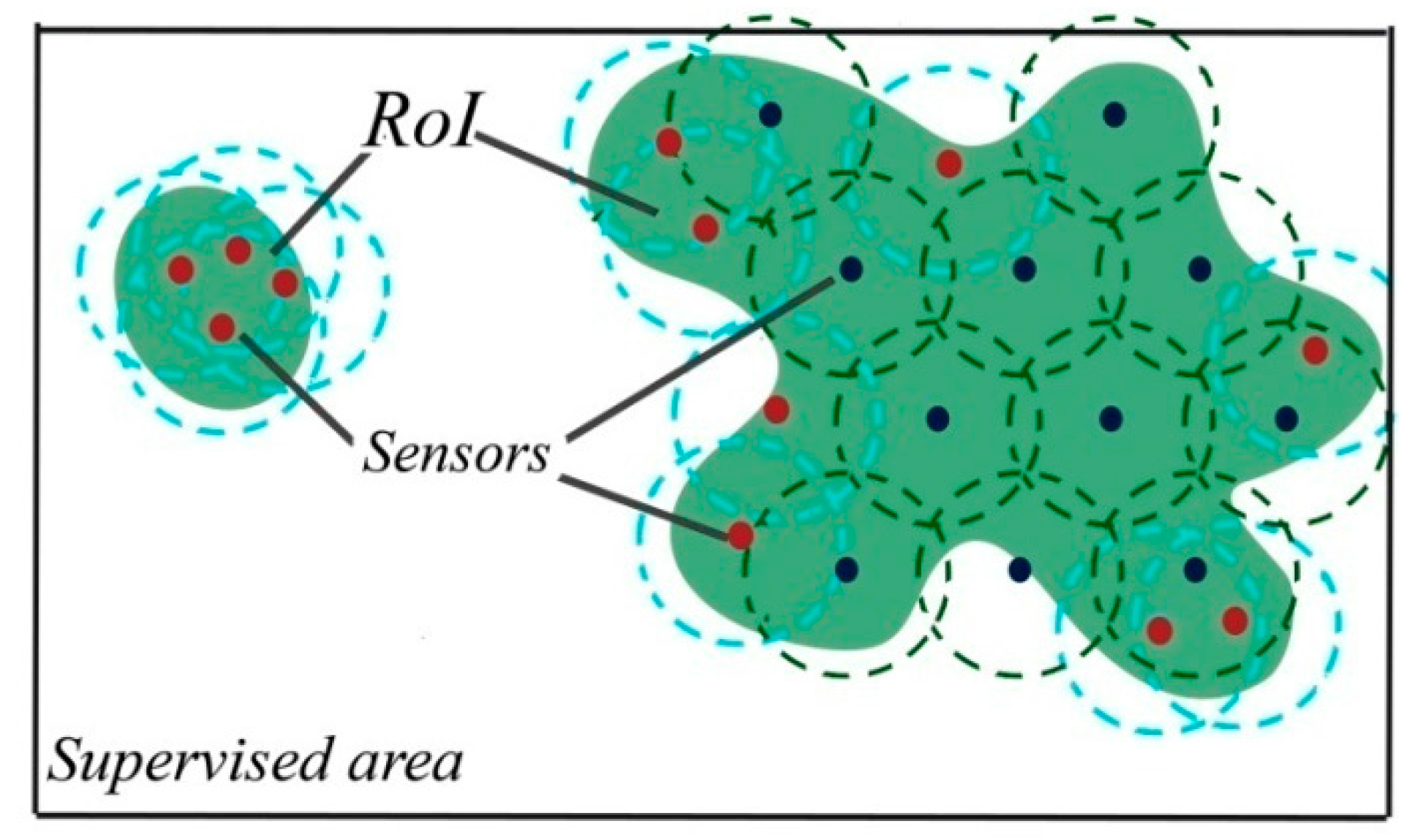
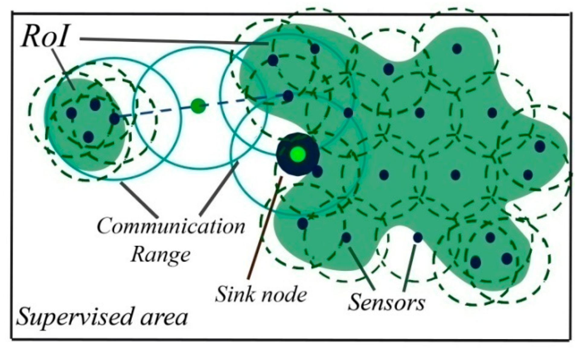
2.1. Preliminary Definitions

There are several types of coverage and connectivity problems in WSN, so depending on the application requirements, we distinguish: area coverage where the goal is to cover an area, point coverage that aims to monitor only a set of points with known locations, and path or barrier coverage, where a barrier must be fully covered to detect any intruders that attempt to penetrate a protected area. An area is fully covered only if every point of the RoI is within the sensing range of at least one sensor node. The network is said to be connected only when every sensor can reach and transmit data to the desired destination. Each and every WSN application requires a certain degree of coverage and connectivity. An area is k-coverage if each physical point in the area is covered by at least k (k ≥ 1) active sensor nodes. The term k-connectivity (k ≥ 1) means that there are at least k disjoint paths between any pair of nodes in the network [8,16].
Based on the type of nodes, WSN can be heterogeneous or homogeneous. Heterogeneous WSN contains sensor nodes with different abilities such as battery energy and sensing range, while in homogeneous WSN all nodes are similar [6,9]. Sensor nodes can be static or mobile. Static nodes are fixed and can’t move after deployment, while the mobile nodes possess all the features of the fixed nodes, and can relocate themselves after deployment [6,17]. Deployment is either deterministic or random. Deterministic solvers can guarantee the best possible sensor placement is found only for a small sized WSN, but they have difficulty with large-scale network cases. By contrast, heuristic solvers cannot generally guarantee the optimal solution but are known to quickly find a near-optimal solution [18]. In [10], the authors developed a classification scheme for sensor node deployment strategies. The primary classification of static deployments is based on non-corona-based and corona-based deployments. Further classification is based on the desired objectives. The first category non-corona based sensor node deployment strategies are categorized as follows:
  • A random-uniform deployment, where sensor nodes are uniformly distributed;
  • Engineered-uniform deployment strategy where the sensor nodes are distributed in an engineered-uniform fashion;
  • Random-Gaussian deployment strategy considers an incremental deployment model such that the number of sensor nodes keeps on increasing near the sink vicinity.
In a corona based sensor node deployment, the sensor nodes are arranged in a circular fashion of radius r with a static sink positioned at the center. The classification of each corona based deployment strategy is based on the required objectives.
  • Engineered Gaussian deployment strategy, where the density of sensor nodes in the first corona is higher than the other coronas, treats the energy hole problem;
  • In the second Engineered corona-based sensor node deployment strategy, the sensor node distribution should achieve the maximum coverage using the minimum number of sensor nodes;
  • For optimized, balanced energy consumption, the third and the fourth categories use, respectively, arithmetic/geometric proportion, to find the optimum number of nodes in Corona;
  • Finally, the engineered corona-based sensor nodes deployment strategy, using relay nodes for transmission that aim to reduce redundant data transmission.

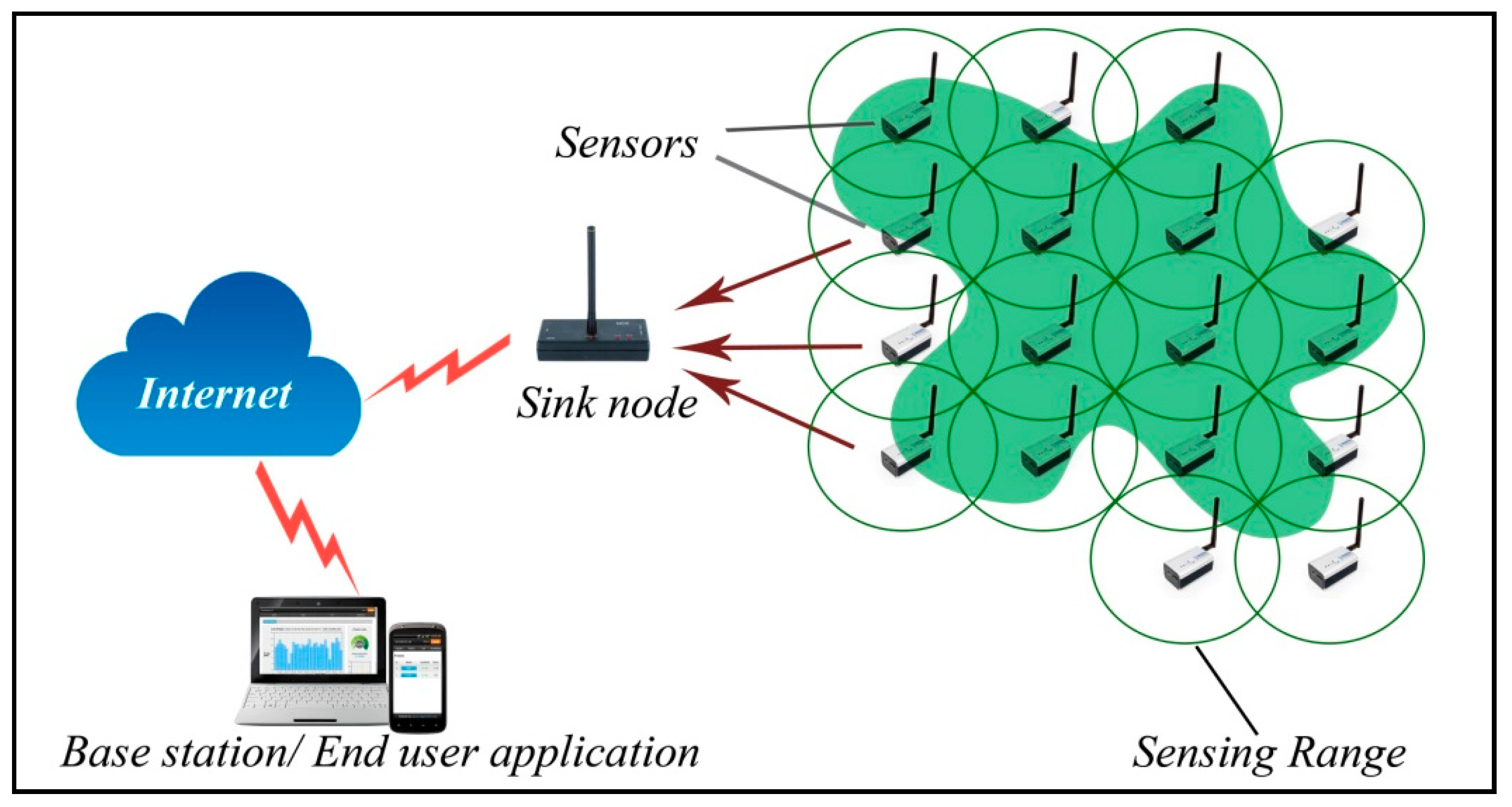
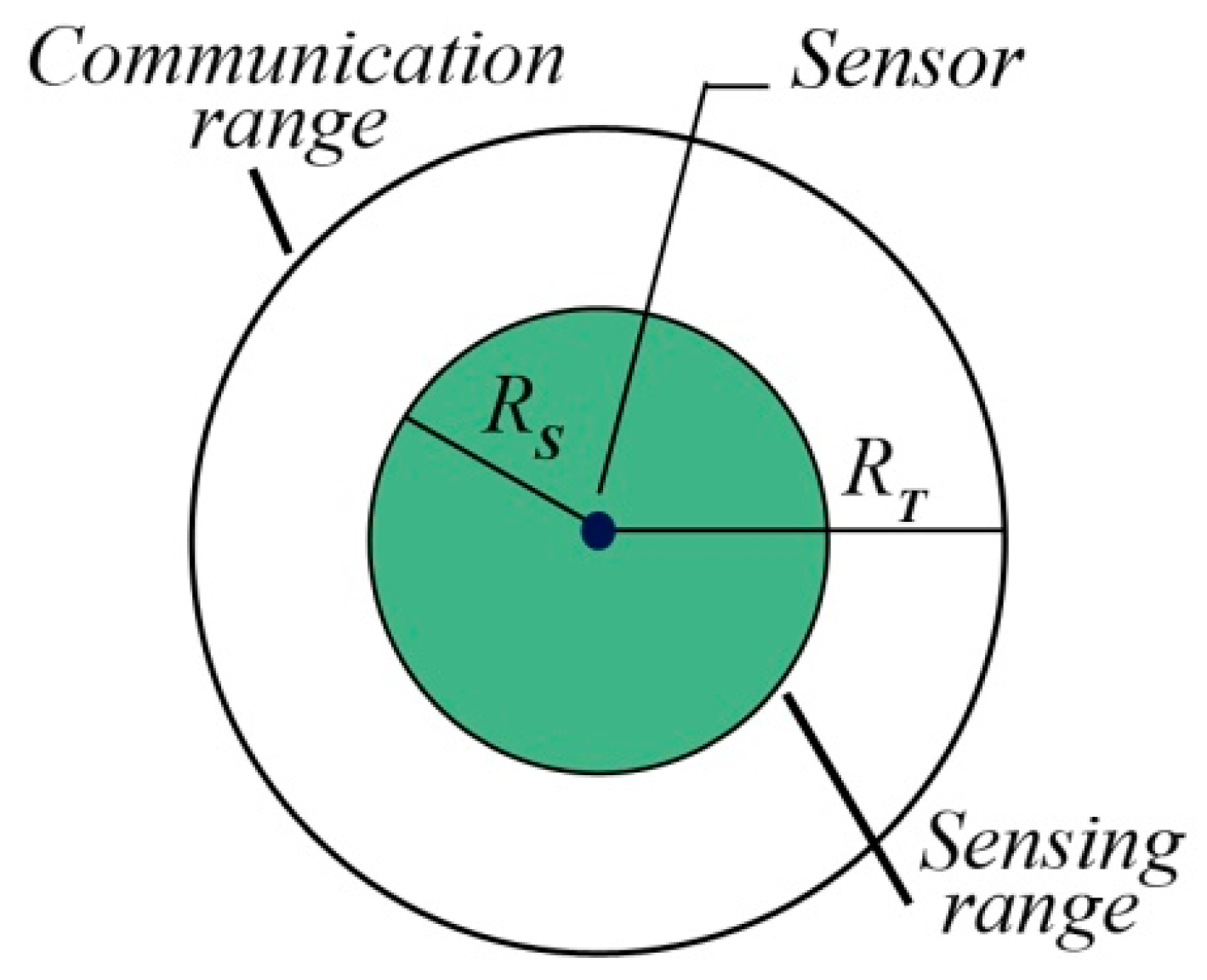
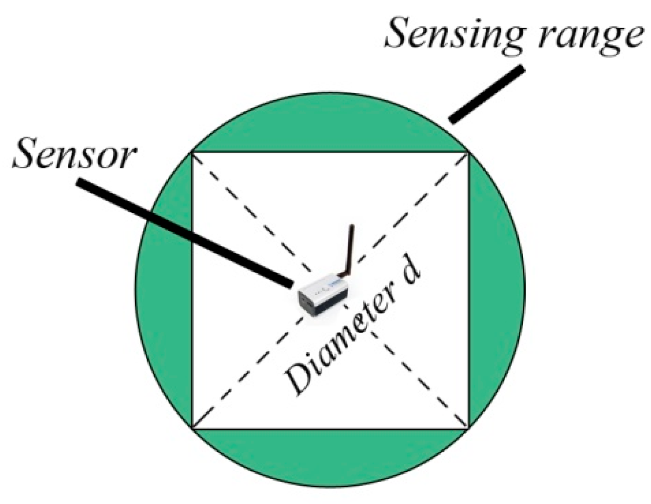
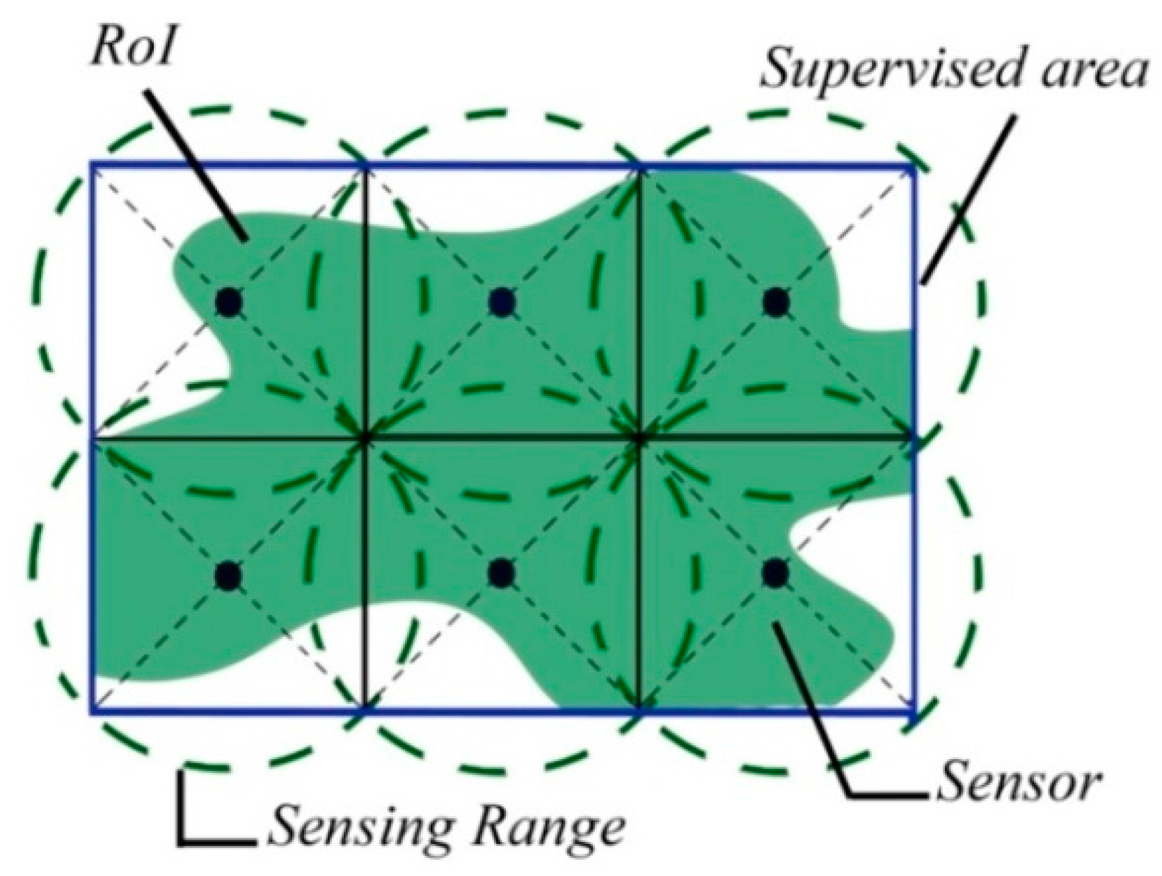
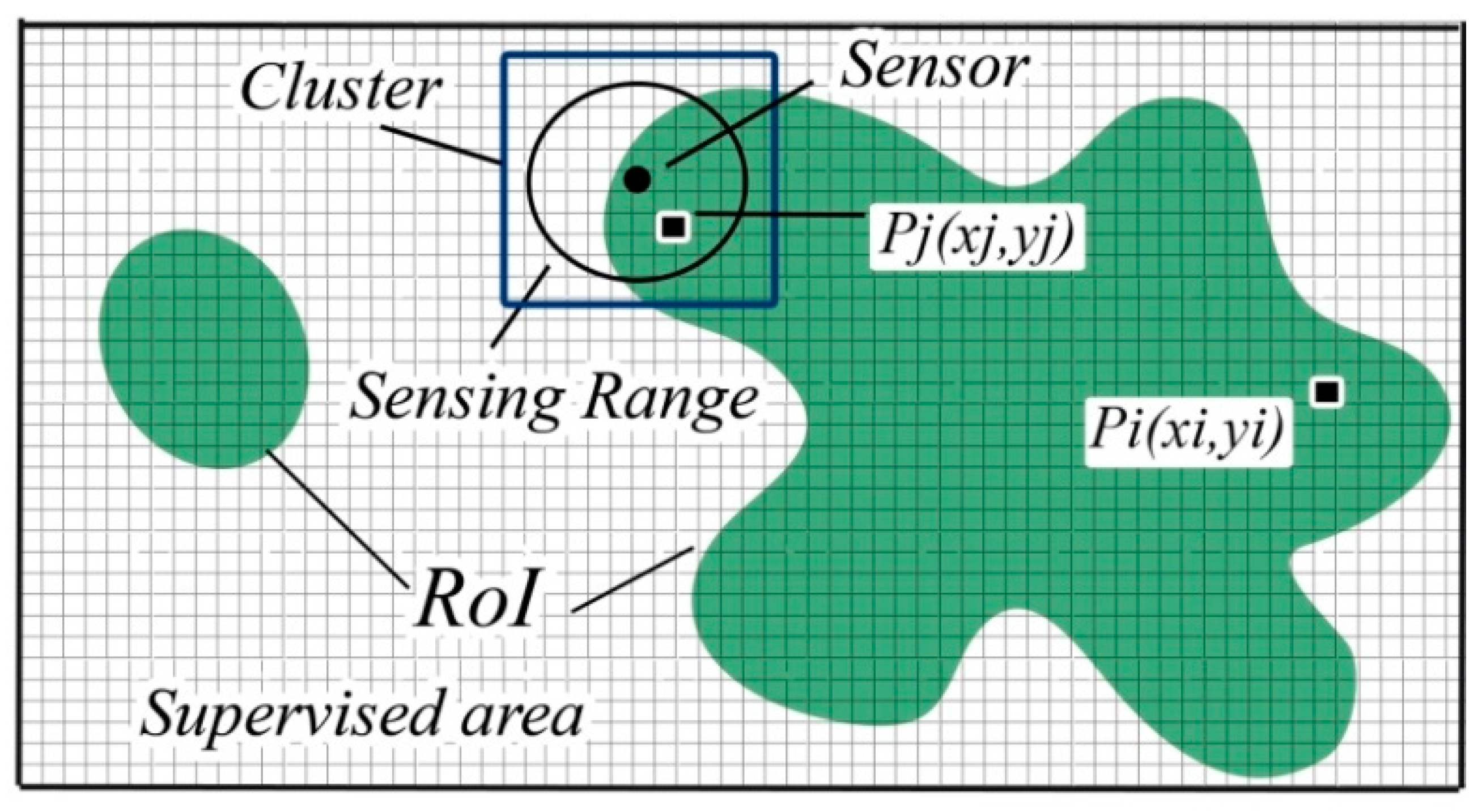
2.2. WSN Basic Concepts

We consider the perception model of a sensor, as shown in Figure 2, where two circles are surrounding the sensor; the first one is the sensing area with R S as the disk radius.   R T   is the radius of the communication range. We consider R T = 2 × R S , it is proven that if the communication range is at least twice the sensing range, it’s a sufficient condition to ensure that a full coverage of a convex area implies connectivity among active nodes [17]. However, this assumption of omni-directional sensing ability does not hold true for some types of sensor nodes, such as cameras, ultrasonic sensors, etc., which have a directional sensing region [8]. Figure 3 shows that if the circular area of the sensing range is a square, the diameter of the circle becomes the diagonal of the square.
Sensors get charged up by batteries, thus they can be used for a limited period. Hence, to make the battery work longer, energy conservation and coverage protocols are required [19]. The event detection probability is inversely proportional to the Euclidian distance separating the sensor from the event. There are two sensor detection models in WSN to find effective coverage. The binary detection model which assumes that there is no uncertainty, and the probabilistic sensing model with stochastic detection [6,20]. A probabilistic coverage better complies with the performance of real sensors in the environment [8]. The binary sensing model is the simplest and most widely analyzed model of coverage provided by a sensor [21,22]. In this model, a sensor detects all events within its sensing range. In this paper, we use the binary detection model shown by Equation (1):
P d ( p s , p e ) =   { 1   if   p e p s < R S 0   if   R S < p e p s
where: P d is the detection probability of an event occurred at position p e , and detected within the sensing range of a sensor placed at location   p s . p e p s   is the Euclidian distance between the sensor and the event.
For simplicity, and as considered in many related works such as [7,9,10,11], we assume omni-directional sensing ability of the sensor, and a binary detection model. The choice of the sensor detection model does not limit the applicability of the proposed approach. The detection model is simply an input parameter to the proposed placement algorithm.

3. Related Work

A wide variety of meta-heuristic methods have been applied to the placement problem, ranging from the genetic algorithm (GA) [23], evolution algorithm with specialized operators [24], particle swarm optimization algorithm (PSO) [25], simulated annealing algorithm (SA) [12,13,14,15], virtual force algorithm (VF) [26], and the virtual force oriented particles algorithm [27]. Other algorithms are analyzed in [16] like the artificial bee colony algorithm (ABC), ant colony optimization algorithm (ACO), and PSO for the sensor deployment problem with the target coverage. An efficient sensor placement optimization model using the Gradient Descent method (GD) was developed in [8]. To evaluate its performance, the proposed method was compared with two optimization methods that were already applied to the sensor placement problem, namely SA and the covariance matrix adaptation evolution strategy (CMA-ES). The results show that GD performed significantly better on larger maps, with much less processing time, while the CMA-ES performed slightly better on smaller maps [8]. SA provides very good and stable results close to GD results on larger maps, and close to CMA-ES performance on smaller maps. These algorithms are adequate only for off-line applications where the sensor nodes need no adaptation after deployment. Based on [10], only the authors in [28], have presented a Corona-based deployment approach using optimum sensor nodes to achieve balanced energy consumption, and to maximize the area coverage and the network lifetime.
As mentioned in [10], each and every approach has its limitations and considers the coverage and connectivity problem to be solved under certain circumstances. Only a few have considered solving the issue of the optimal number of nodes while optimizing coverage and connectivity. Based on [29], estimating the number of nodes can be done basically by dividing firstly the network area into a number of subsets of nodes, called cover sets, as shown in Figure 4. If the cover sets are disjointed, one sensor node can be present in only one cover set. As demonstrated in Figure 3, the diagonal is the diameter of the circular area of the sensor d   = 2   ×   the   radius   of   coverage . Since this diagonal divides the square into two isosceles triangles, then the sides of the square can be easily calculated using trigonometric functions. Sin θ= perpendicular/hypotenuse = L/d; where θ = 45°. So, the side of the square is   L = d × sin 45 ° . Assuming the area to supervise is a square with sides A and B. Thus, the number of nodes is decided N = A L   ×   B L .
Generally, this method is used to determine the initial number of sensor nodes, and based on the results obtained by the sensor deployment method, we can choose to increase or to decrease the number of nodes to deploy. In Figure 4, the area to supervise was divided into six cover sets, which means that six nodes are needed to cover the area. However, this method is far from providing the optimal coverage, connectivity, and network cost. Node deployment is simply a matter of choosing the best locations for the optimal number of nodes to cover the RoI. In addition, to calculate the node placement, composite factors, which are combinations of environmental factors, should be considered such as the relationship between the sensing range, the communication range, and the node deployment type [30]. Our approach is based on the SA algorithm, because, based on [12,13,14,15], it provides a good and implementable response for network design and better energy efficiency by organizing the sensor nodes.

4. WSN Deployment Approaches Based on the SA Algorithm

In reality, temperature is the controlling mechanism used to convert material from a high energy state into a low energy, in solid conditions. This process is imitated in SA, where the temperature controls the number and spread of accessible solutions from a given solution in the search space. SA begins with a high initial temperature to allow a random walk in the search space. As the temperature gradually decreases, the system becomes more focused, only allowing moves in the search space which improve the performance of the solution. The process terminates when a temperature close to zero is reached [8]. If the temperature is not high enough, the SA approximates a local optimum, instead of the global optimum of the objective function.
In our approach, we use the simulated annealing algorithm as an optimization method in order to find the optimal deployment. Two approaches were presented in [13] and in [14] using the same algorithm. In those approaches, the authors assumed that each point of the ROI is different from another since each point has its own importance, thus they used the term “interest” to refer to the importance given to supervise a point. In the first one, the objective was to find the optimal topology guaranteeing coverage, connectivity, and a maximum interest with a fixed number of nodes. In the second one, the objective was how to deploy a fixed number of nodes with the purpose of providing coverage, a maximum interest, and ensuring connectivity with the minimum number of hops between all nodes and the sink. Our goal is to find the minimum number of sensor nodes with the best topology providing the maximum interest with at least 1-coverage and 1-connectivity. In the approach presented in [13], the objective function computes the value of the interest collected by every set of nodes, guarantees connectivity, then provides the optimal topology, ensuring the maximum interest in the area.   {   If   f K ( X * ) f K ( X ) ,   with   f K ( X * )   the   new   output   of   f K ( X ) } the function’s output is saved to C, otherwise it’s equal to the optimum solution stored in C. As shown in Equation (2) this function has two sub-functions. The first one computes the minimal distance between nodes and the second calculates the joint interest collected in all the regions of nodes.
f K ( X ) =   { γ . f min   ( X )   +   f s   ( X )   ,   i f   X   i s   K survivable C ,   otherwise
where: X is a set of N nodes. X= ( x 1 ,   x 2 , x i x N ) R 2 .   C is a constant ensuring that only survivable solutions will be accepted.   γ   controls the dispersion of nodes, a small value makes sensor nodes to stick together, a larger one disperses nodes regardless of the importance of the RoI. f s ( X ) is the sub-function representing the joint interest of the sensor nodes and penalizes coverage overlapping: f s ( X ) =   i   = 1 N α i . area ( S i ) − β. area i   = 1 N S i . α i   is the given importance of location x i , β a penalty on sensor coverage overlapping and r s is the sensing range. S i denotes the open ball with center x i and radius r s , and δ ( x * , x i ) =   x * x i is the Euclidean distance between points   x *   and   x i . S i = { x * Z :   δ ( x * , x i ) r s } . f min ( X ) : Measures the minimum separation between a sensor whose position is shifted d units in R 2 and all the others:   x i , x j   X,   i ≠ j f min (   ( X \   { x i } ) { x i + d } ) = min( δ ( x i + d , x j ) )
X is K-survivable if for any simultaneous failure of K nodes in X, every surviving node x i lies at least within the coverage of another surviving node   x j , and each one must be able to communicate with the sink either directly or indirectly. Maximizing f K ( X )   implies the maximization of   f min ( X ) , and ensures that the set of nodes of the solution will be separated by the maximum distance allowed. The sub-function   f s ( X ) computes the interest collected and penalizes the overlapping which occurs by the intersections of the sensing regions of the nodes.
In [14] another approach was developed to provide maximum coverage with improved connectivity properties, allowing a minimum number of hops between all nodes and the sink. Based on the objective function in [8], and as shown in Equation (3), a new sub-function was added to compute the average of the number of hops between all the nodes and the sink. In this case, maximizing the objective function will minimize the function of average hops.
f K ( X ) =   { γ . f min ( X ) σ .   f α ( X ) +   f s   ( X )   ,   i f   X   i s   K survivable C ,   otherwise
f α ( X ) is the function of the average number of hops defined by Equation (4) as follows:
f α (   X { x i , s } { x j + d   }   ) =   1 N 1 × j   = 1 N 1 j   =   1 p j nbr _ hops ( s , x j ) p j
where, s is the sink node, p j represents the total number of paths between s and x j , d is an arbitrary distance oriented in a random direction, and nbr _ hops (s, x j ) computes the number of hops between the sink and the node x j . While the first algorithm based on SA in [13] tries to optimize deployment only by maximizing coverage, the second approach in [14], searches for the optimal placement of nodes by maximizing coverage while ensuring a k-connected graph. Moreover, both approaches consider a fixed number of sensor nodes.

5. Model Formulation and Description

5.1. Model Formulation

Assuming that the field of interest is a two-dimensional square region with area Z = A × B/Z R 2 , and the network to be homogenous, N sensor nodes are deployed in the target region Z, and the location of sensor i is denoted x i . We consider that every colored pixel represents a point with interest, a point has no interest when its color is white. A set of points with interest represents a Region of interest as demonstrated in Figure 5. We need to deploy an adequate number of sensor nodes X = ( x 1 ,   x 2 , x N ) that will fulfill at least 1-coverage and 1-connectivity. Based on the triangular deployment grid, sensor nodes are deployed line by line while the first is placed randomly on the map. Each node that collects an interest different than zero is selected and saved. Using the gradient method, all sensor nodes on the RoI boundary are detected and set to seek more interest. Finally, the joint interest collected by the given set of sensor nodes X is calculated.
With every iteration, the minimal distance between sensor nodes, which is the distance between each node and its first-degree neighbors’, is updated, and the adequate number of nodes is recalculated. If the recalculated joint interest is equal or greater than the previous one, the positions are updated. In order to minimize the processing time, the collection of interest for each sensor node is done using a clustering technique so the search will focus on a cluster which is a square, instead of the whole supervised area. Each cluster’s center is a sensor node position. Let (Xi,Yi) be the Cartesian coordinates of a point Pi, and (Xs,Ys) the sensor node coordinates. The cluster is defined as follows   C k = {   ( Xi , Yi ) ² / | Xs Xi |     R s & | Ys Yi |     R s } .
The new objective function described in Equation (9) is developed based on Equation (2) developed in [13].   {   If   f ( X * )     f ( X ) ,   with   f ( X * )   the   new   output   of   f ( X ) } the function’s output is saved to C, otherwise it’s equal to the optimum solution stored in C. We updated the interest function given by Equation (8), and we added new sub functions given by Equations (5)–(7). The new sub functions are defined, as follows:
f G ( X ) =   f ref ( x , y ) . u
f TX ( X ) =   x i + ( k . step . x i x j d max   )
f N ( X ) =   A d min . B d min
where, the gradient function   f ref =   f ref x ,   f ref y and ( f ref ) is the class function, the class of covered point is {1}, while uncovered point has {−1}. u is a unit vector. d max is the distance between unconnected nodes x i and x j . d min is the distance between close nodes. k is the number of nodes needed to achieve connection, step is the distance between new nodes: step = a × R T .
f S ( X ) = i   = 1 N [ α i . area ( S i )   area ( j   =   i N S j ) ]
f ( X ) =   {   f min ( X ) +   f S ( X ) + f G ( X ) + f TX ( X ) f N ( X ) C ,   otherwise
where: X is a set of N nodes. C is a constant ensuring that only survivable solutions will be accepted.   f min ( X ) denotes the minimum distance between sensor nodes given by Equation (1) where d = d min and increases by ν in every iteration.   f S ( X )   is the sub function that collects the interest detected by every node in the area given by Equation (8). f G ( X ) , given by Equation (5), is the sub function that allows sensor nodes on the RoI boundary to move with µ in the right direction to maximize the collected interest. By using the derivate of the reference function in the direction of i and j . f TX ( X ) , given by Equation (6), one finds the minimum number of nodes needed to ensure connectivity. f N ( X ) is given by Equation (7), to define the number of the nodes to deploy.
In Algorithm 1, the number of iterations T depends on the application parameters, such as the size of the map, the sensing range, the initial minimal distance of deployment d 0 , and the final desired distance d N between a sensor node and its first-degree neighbors. It can be calculated as follows: n =   ( d N     d 0 ) /   ν , with ν the added value to the actual minimal distance between nodes each time. We initialize the distance between close sensor nodes with R S , then we calculate the number of nodes needed to monitor the whole area. Since the nodes are too close to each other and overlapping between sensor nodes is penalized, the maximum value of the joint interest is achieved in the first iteration, and full coverage and connectivity are ensured. This method has allowed us to approach a multi-objective optimization problem by solving a mono-objective optimization problem, which maximizes the joint interest. The other objectives can be automatically reached by an upgrade of their values. Thus, the proposed algorithm allows finding the maximum joint interest that can be collected by all sensor nodes in the network while minimizing their number, and maximizing the distance between close nodes.
Algorithm 1: Gradient—SA Hybrid Algorithm for Sensor Deployment
1. T = T0, is the initial temperature and d =   d 0 the initial distance of deployment. ν and µ denote respectively the added value to the actual distance of deployment d and the transition value for nodes at the boundary.
2. Let compute the initial number of nodes,   N 0 = A d 0 × B d 0
X 0   = {x1, x2,…, xN0 } (i) corresponds to the index of the current node. Initial interest function value is f S ( X 0 )   = 0 and   f S ( X ) = 0 .
3. While T > 0
\\Let distribute nodes line by line and save those with a collected interest value Si ≥ 0, then compute   f S ( X ) . The first position is chosen randomly.
3.1 While k < sensor nodes on x-axis,
3.1.1 While j < sensor nodes on y-axis
3.1.1.1 Define the cluster
3.1.1.2 Calculate the collected interest Si per node then the joint interest.
3.1.1.3 If Si > 0 then xi ϵ (X);   f S ( X ) =   f S ( X ) + Si End
3.1.1.4 Shift the sensor position horizontally by ν;
3.1.1.5 Update j
3.1.1.6 end
3.1.2 Shift the sensor position vertically by ν . 3 / 2 ;
3.1.3 Update k
3.1.4 End
\\Let search for sensors on the RoI boundary, shift their positions and calculate the sum of collected interest of sensor nodes.
3.2 t =   ( d Rs 4 ) / μ , is the number of iterations needed for a node to move from its position on the Roi boundary until approximating its neighbour by Rs/4.
3.3 While t > 0
3.3.1 While I < N sensor
3.3.1.1 Detect sensors on the RoI boundary S E
3.3.1.2 Shift S E positions by µ using f G ( X )
3.3.1.3 Define the cluster then calculate the collected interest
3.3.1.4 End
3.3.2 Calculate the joint interest   f S ( X ) ;
3.3.3 t = t     γ
3.3.4 End
3.4 If f s (X0   f s (X) ≤ Q then f S (X0) = f S (X) End;   f S ( X ) = 0
 \\Q is the accepted tolerance: For 100% coverage Q = 0
3.5 Let detect unconnected nodes, and add nodes by using f TX ( X ) .
3.6 Upgrade the values of the functions   f min ( X ) and f N ( X )
3.7 T = T     δ.
3.8 End

5.2. Model Description

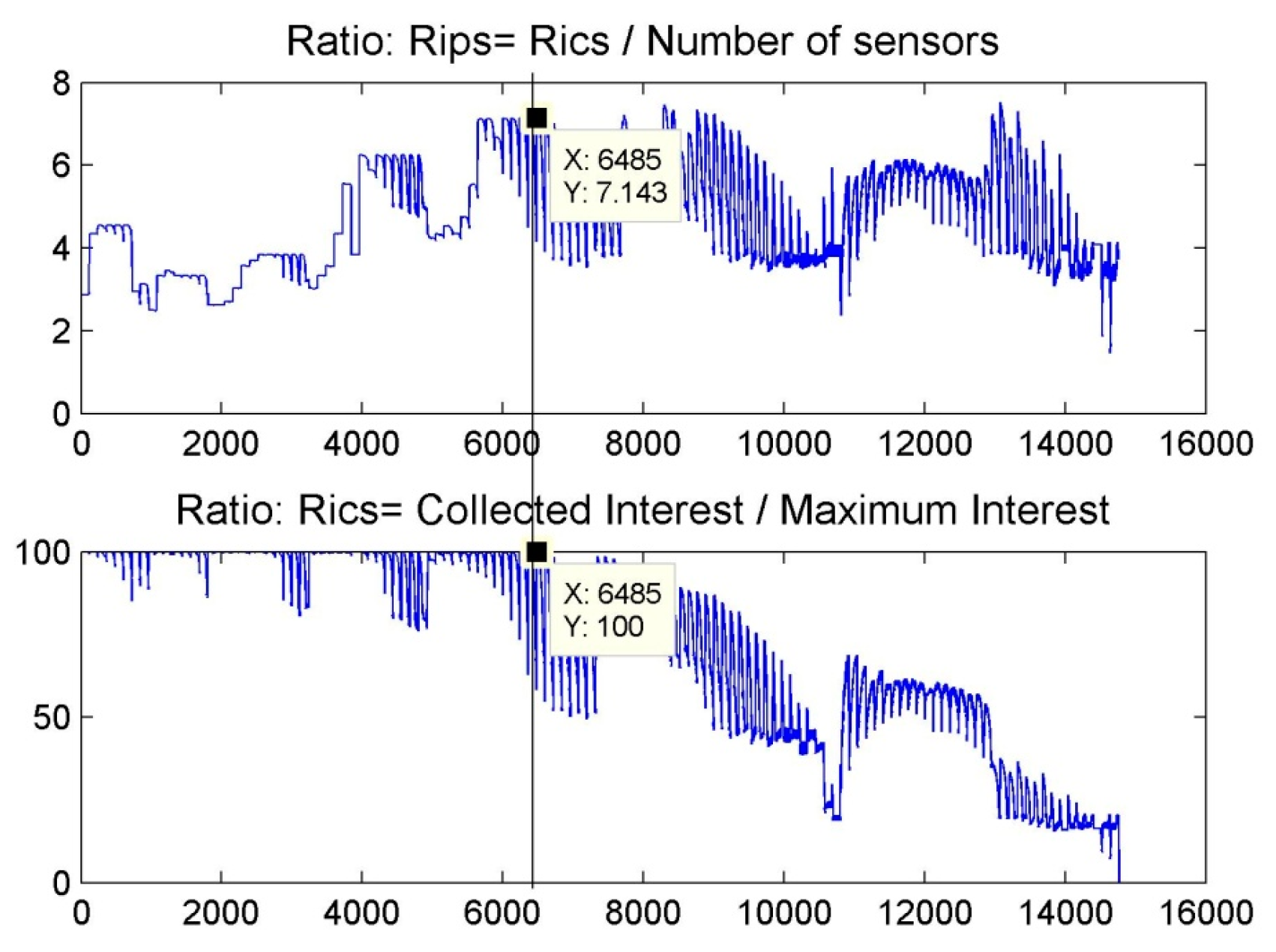
5.2.1. Step One: Searching for Interest

For the purpose of simplifying the calculation and minimizing the processing time, we seek the interest that should collect every sensor only within a cluster where the majority of the points are within the sensing range of the sensor. This cluster is a square, with L as its length L ≥ 2 × R S , and the sensor position as its center.
We use the triangular grid deployment technique, because based on [10], when R T   =   2 × R S the triangular lattice is the best deployment pattern.
Firstly, we began by putting sensor nodes line by line, d min is the distance between nodes. Assuming that for the initial deployment d min =     d 0 , the initial number of nodes to deploy is N 0 = A d 0 × B d 0 . When d min increases, the number of sensor nodes N to deploy decreases. Figure 6a,b show this process at two different time steps. For each deployed sensor, we calculate the collected interest. In Figure 7, nodes in gray gathering no interest are removed, then the selected nodes collecting information are chosen to be saved (Figure 8).

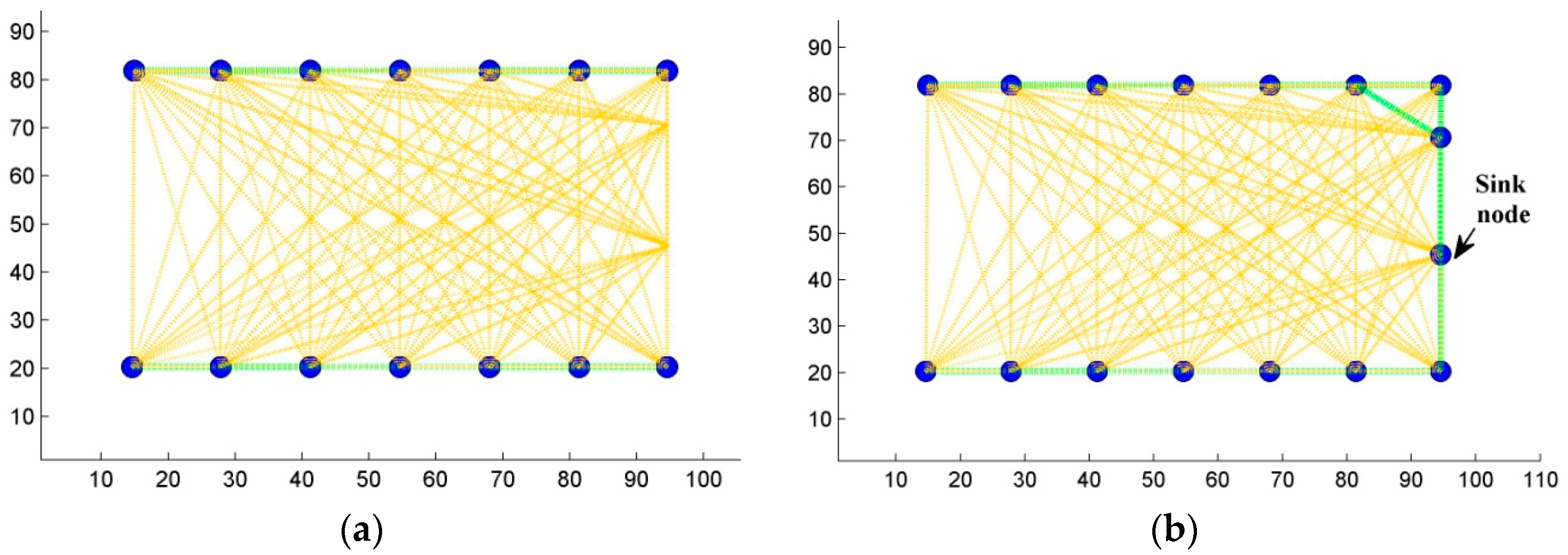
5.2.2. Step Two: RoI-Boundary Sensor Optimization

The objective of this step is to move nodes placed on the boundary, in the right direction to collect more interest. We decided to use the gradient method. Two classes are defined and represent the class matrix. Class {1} represents points with interest, class {−1} represents points without interest. After we use the clustering technique and creating the reference matrix, we apply the gradient function so we can detect nodes on the boundary, and secondly decide the movement direction to seek more interest. Figure 9a,b show an example of this process where blue sensor nodes are the boundary nodes that should be relocated.
At each step, the gradient of the reference matrix is calculated and the sensor location is updated to make a small step in the right direction to gather more interest. The joint interest will be recalculated for the new solution, and this step is repeated until the maximum number of iterations is reached. When the distance between two nodes is less than the sensing range, in our case Rs/4, the sensor on the RoI boundary is deleted. In this case, the maximum number of iterations needed for a node to move from its position on the Roi boundary until approximating its neighbor by Rs/4, should be at least t =   ( d Rs 4 ) / μ , as already described in the pseudo-code. Figure 10 shows that better sensor positions were found after applying this method to the design presented in Figure 8.Distance is an important factor for sensing. When the distance between the node and the event increases, the sensing power decreases and battery consumption increases [30,31]. One of the most important requirements of WSNs is to reduce the energy consumption [32,33]. Hence, this technique allows not only seeking better positions for nodes to monitor more events but also getting close to the RoI so energy saving can be achieved.

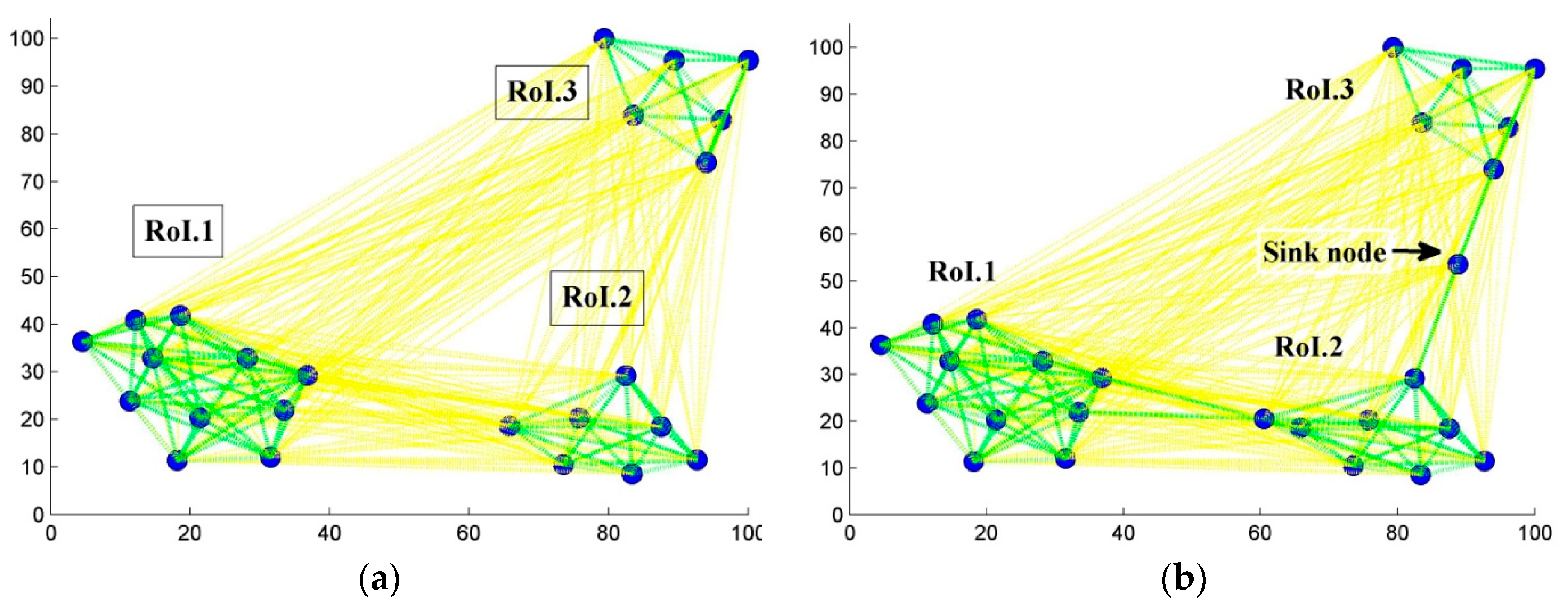
5.2.3. Step Three: Ensuring Connectivity

In this step, we define the unconnected sensor nodes and the minimum number of sensors needed to achieve full connectivity. We assume that the sink node connects the whole network to the base station. Firstly, we sort X, the set of nodes, in ascending order according to the Euclidean distance of these nodes to point zero. Secondly we calculate the distance of every sensor to all the others, only in one direction, as shown in Table 1, where d i , j is the Euclidean distance between nodes x i , x j , then we seek the minimum distance between nodes line by line.If the minimum distance d i , j > 2 × R T , new sensor nodes are to be deployed between nodes x i and x j and Equation (6) is used to calculate their number.
Figure 11 proposes a WSN design that collects a maximum interest and ensures full coverage and full connectivity. The sink node is decided in a way to avoid network congestion.

6. Results and Discussion

Using MATLAB, we tested our approach on a 100 × 100 pixel picture that represents the distribution of the interest in a given area. The RoI is colored in yellow, green pixels represent no interest. Based on the developed equation given by Equation (9), the algorithm computes the collected interest, and optimizes the objective function f (X). We define two parameters that can confirm if our approach chooses the optimal topology. The first one is the ratio of interest   Rics =   Calculated   interest / Maximum   Interest , and Rips = Rics / Number   of   nodes is the second ratio that shows the average of the interest collected per sensor. Rips is at its minimal value when the area is over-covered, or in other words, the number of deployed nodes is more than sufficient, since the same interest is collected while the number of nodes decreases in time, which makes the Rips ratio increasing in time, meaning that the average of interest calculated per each node increases with time. Otherwise, if the area is less covered, Rips reaches its maximum. Two scenarios are presented where the coverage problem is to be solved while finding the adequate number of nodes. The first one is the case of the area coverage problem. We define three regions RoI.1/2/3 within the area to supervise, at least 97% of the joint interest must be satisfied. The second case is a barrier coverage problem where 100% of the joint interest must be collected. Then a comparison is made between our results and those obtained in [3].

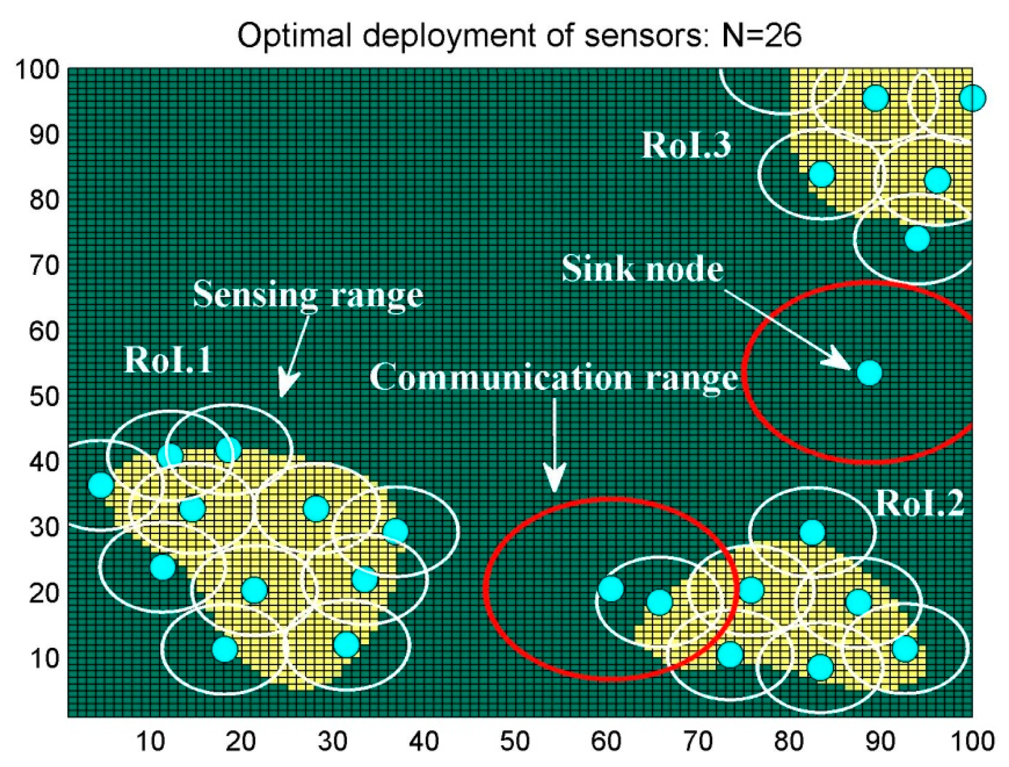
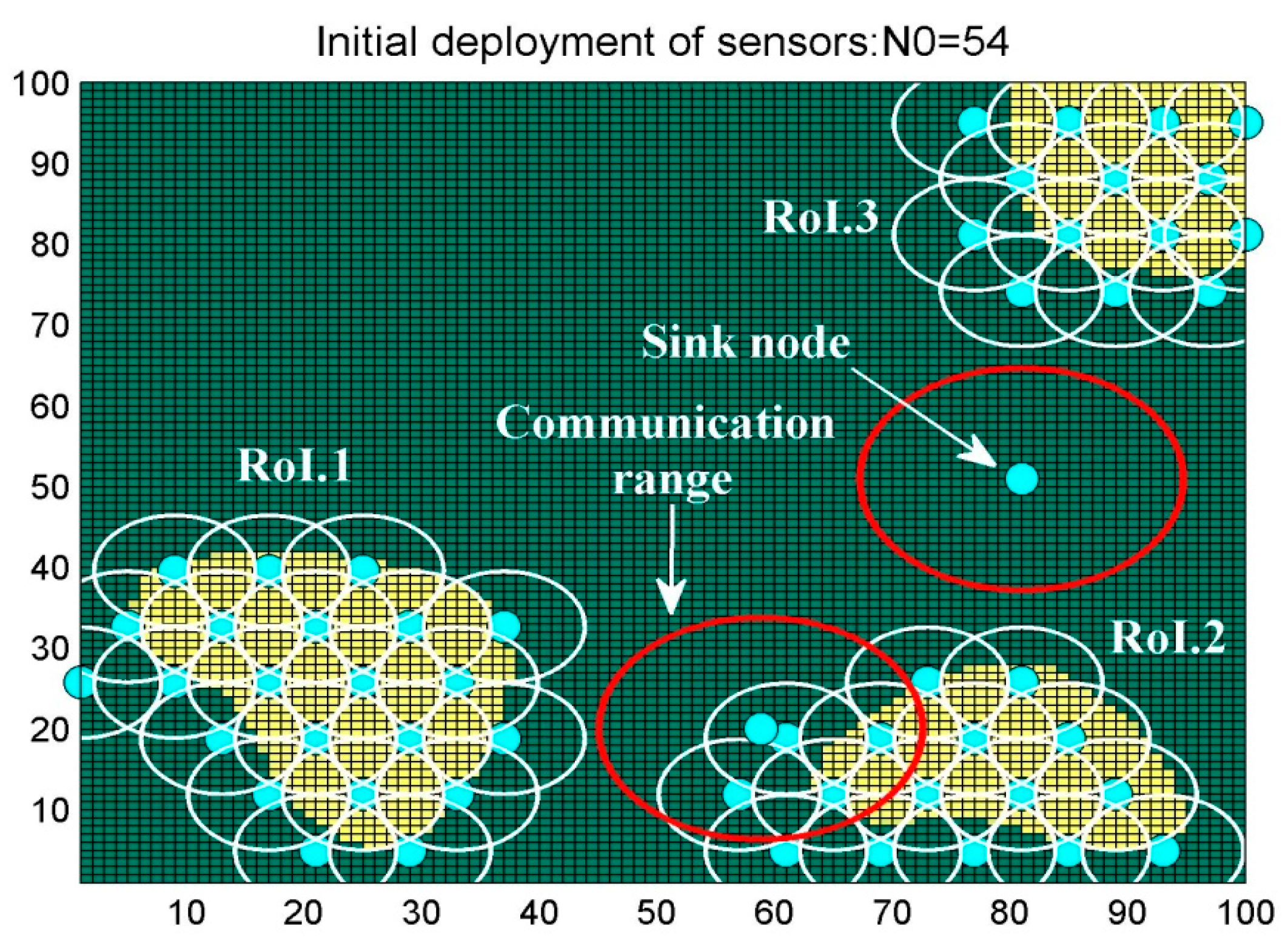
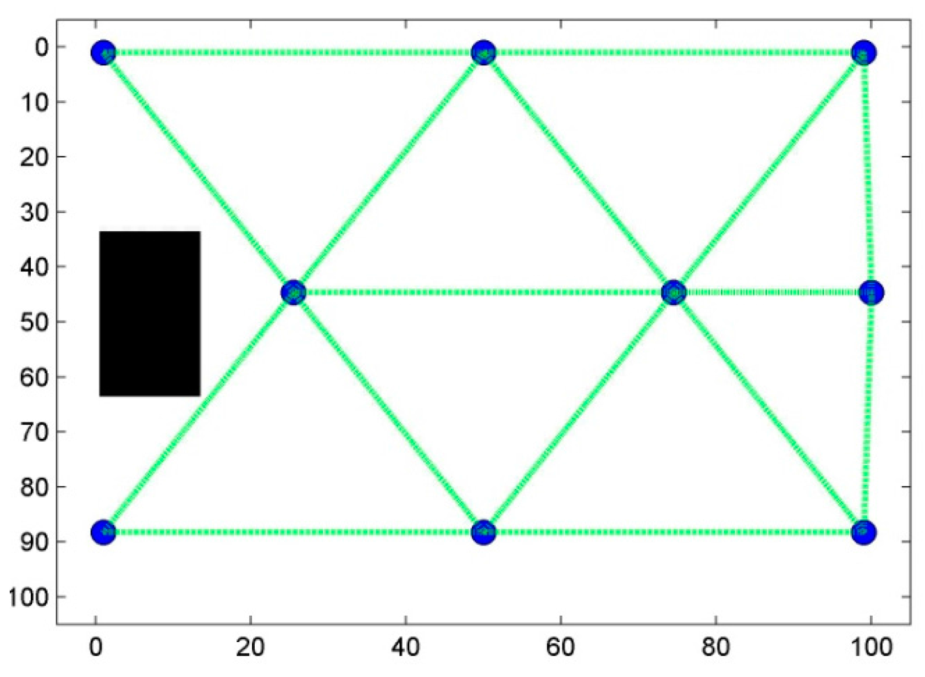
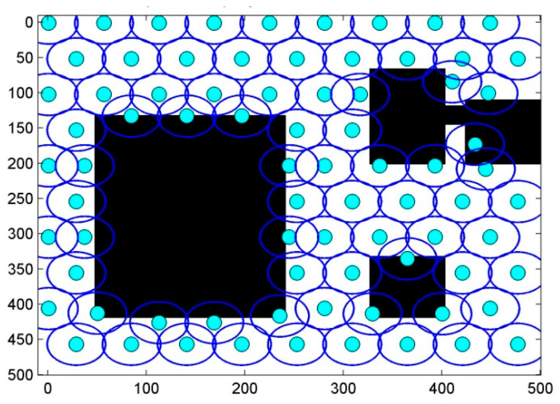
6.1. Scenario 1: Area Coverage with RoI.1/2/3

These simulations had been performed with precise parameters which provides better performance:   d 0   =   R S the initial distance, ν = 0.5 the distance to add between nodes after every iteration, µ = 0.05 the transition distance for sensor nodes on the boundary, R S = 7   the sensing range and the communication range   R T   = 14 .
Initial deployment is illustrated in Figure 12. The Initial number of sensors needed to monitor the area is calculated based on the initial distance   d 0 , N 0 = 54. The model decides to add one sensor between RoI.2–RoI.3, and another one between RoI.1–RoI.2, so full connectivity can be achieved. After many iterations, the algorithm decides whether to save the proposed design or not based on the value of the objective function. At the end, the best topology was found at iteration 6673, shown below in Figure 13.
Figure 14a illustrates the network before ensuring connectivity. Sensor nodes within the same RoI are connected, and there is a bi-directional link in green between them as they are within each other’s communication range, while nodes from a different RoI are isolated as shown by yellow links.
Figure 14b is an illustration of the network after ensuring the connection between all sensor nodes and defining the sink node. Full connectivity is achieved, as demonstrated by all the green links passing through all sensor nodes. Figure 15 illustrates that the required degree of the joint interest is satisfied using only 26 nodes instead of 54 nodes used in the first deployment, and it shows that the best deployment was found at iteration It = 6673, where the topology provides a joint interest of 97.09% coverage ratio, with a minimum number of sensor nodes. During the first 400 iterations, the maximum joint interest was approximately satisfied and Rips values were increasing while the numbers of nodes were decreasing, meaning that the area was over-covered. The processing time of the application was around 60 s but only if the first and the optimal deployment topology are displayed, otherwise it exceeds 10 min.

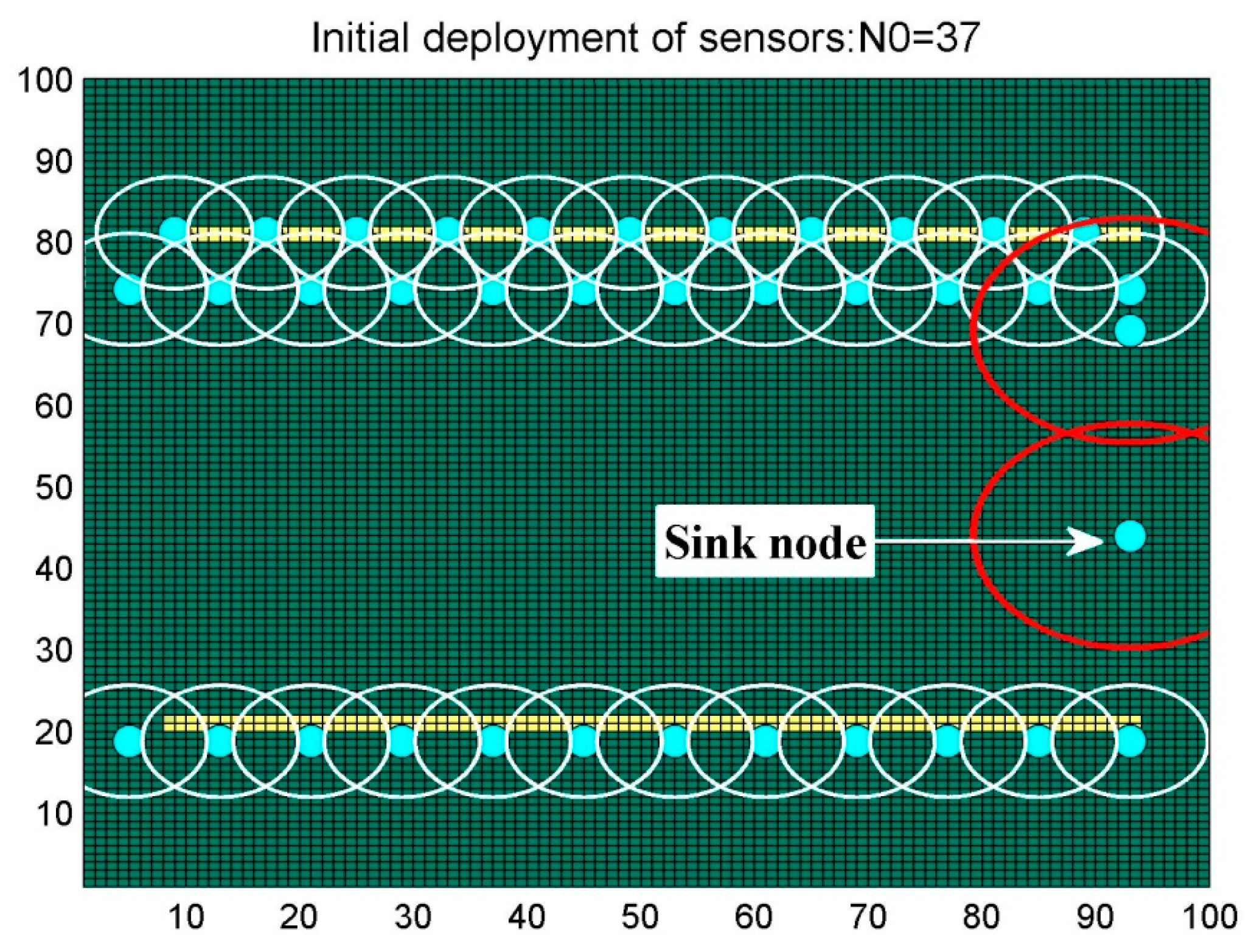
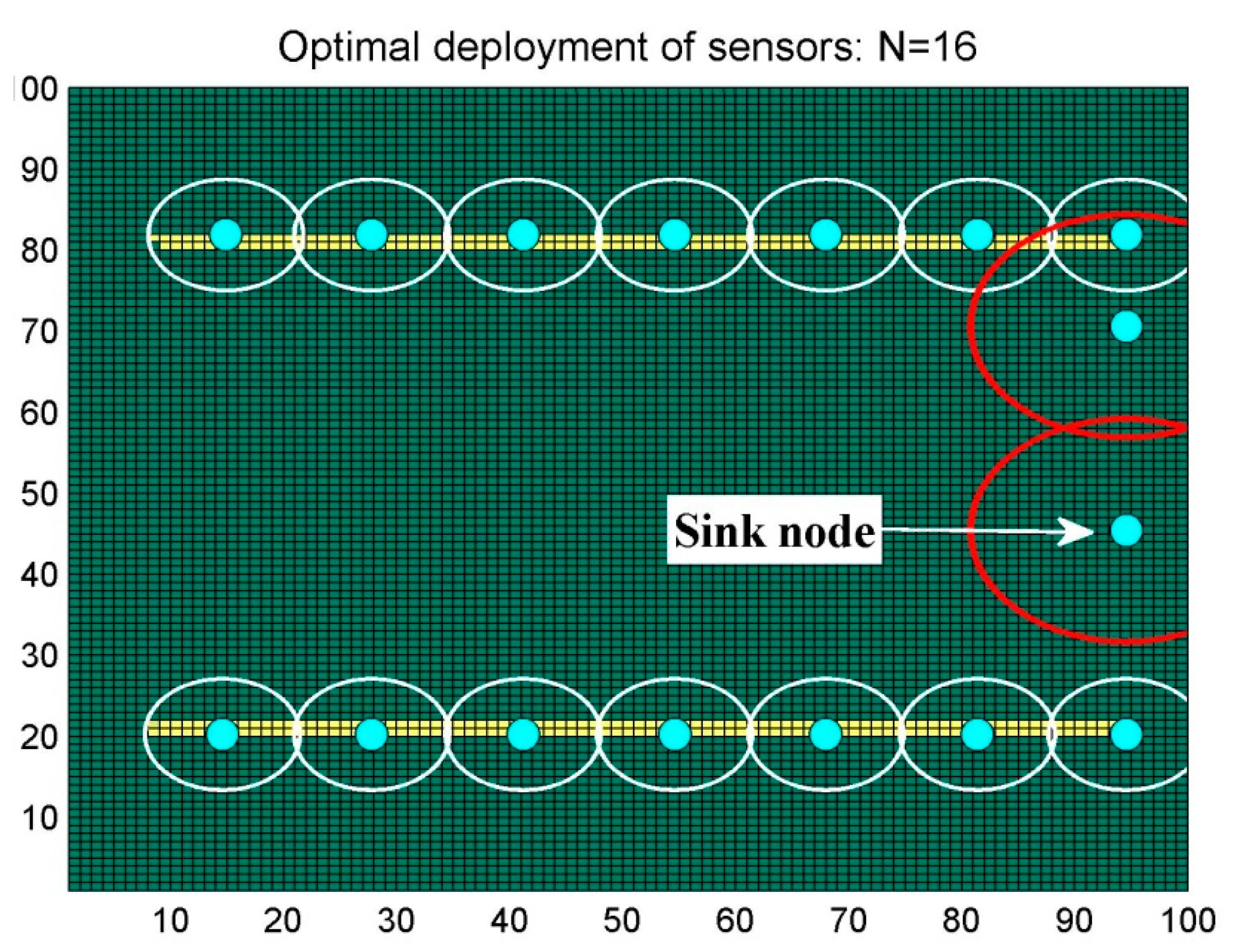
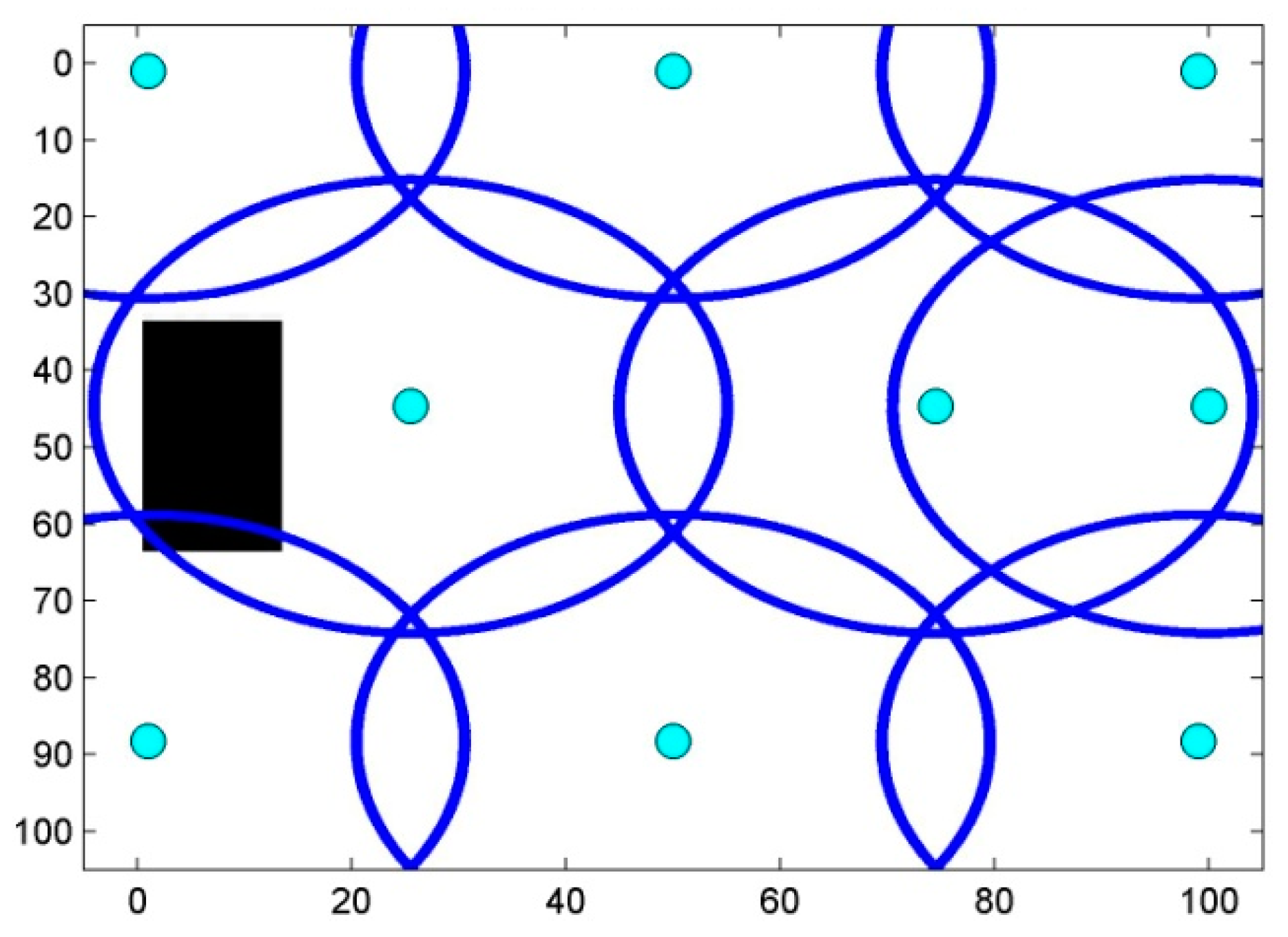
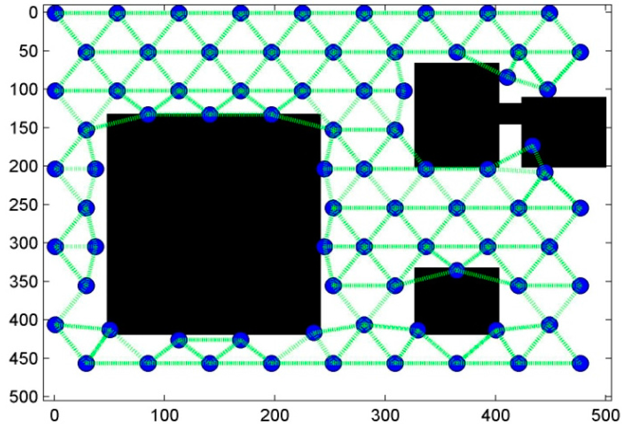
6.2. Scenario 2: Barrier Coverage

In this Scenario, we monitor a barrier within the area in order to detect any intruders. We used a picture with 100 × 100 pixels, where the barriers are colored in yellow. In this simulation, we use the same parameters: µ = 0.05,   d 0 =   R S   ; R S = 7   ;   R T   = 14 ; except for ν = 0.1, so better performance could be achieved.Figure 16 shows the initial deployment with N 0 = 37. After optimization, the algorithm found the best deployment of nodes at iteration 6485, achieving the collection of the maximum joint interest with N = 16 nodes, as illustrated in Figure 17.
Figure 18a shows the network before guaranteeing connectivity. Two unconnected groups of sensor nodes are detected. Nodes within the same group are connected as demonstrated by green links. Otherwise, nodes from different groups can’t communicate with each other as shown by yellow links. Figure 18b shows a fully connected network as demonstrated by the green lines linking all nodes so they can reach the sink node.
Figure 19 demonstrates the Rips and Rics values for different designs. The optimal topology was detected at iteration 6485, where 100% of collected interest is reached, while full coverage and connectivity are granted. Besides, the best average of collected interest per sensor is achieved, proving that the algorithm has chosen the best topology between all designs, ensuring that the area is not over- or under-covered.

6.3. Comparisons

In order to compare our method to the GD method developed in [8] and the CMA-ES method, we used an area with the same properties as the map of the Campus of Laval University, Canada used in [8]. The same sensing range is defined, however, in our case, the sensing area is considered to be isotropic, while in [8] the sensing angle is between 60° and 120°. This constraint shows no limitations since the isotropic sensing model plays the role of the directive sensing model. We defined two images. The first one represents a small map with dimensions of   100 × 100 pixels, named UL-A, and the second represents a larger map with dimensions of   500 × 500 pixels, named UL-B.
Black pixels are points with a very low interest and they are assumed to have no interest. The white pixels are points with interest. For better results, we define ν = 0.1 and µ = 0.1. Figure 20 shows the optimal placement of sensor nodes on the first map, UL-A. 100% coverage is reached and the maximum interest is achieved. Figure 21 demonstrates that full connectivity is reached.
On the second map, UL-B, the optimal deployment described in Figure 22 achieves 89.48% of the joint interest. The proposed topology ensures full connectivity as shown in Figure 23. Table 2 regroups the results of three methods, the proposed model, the GD algorithm developed in [8], and the CMA-ES algorithm used in [8].
Table 2 proves that the proposed algorithm provides competitive results especially on smaller maps, where the maximum coverage value is achieved with fewer sensor nodes. On larger maps, the algorithm provides good results since it offers approximately the same coverage, but with more nodes than is needed in the other methods. In both cases, the processing time of the proposed algorithm is far less than that of CMA-ES.

7. Conclusions

In this paper we propose an optimization model to solve one of the major concerns of WSN, the sensor placement problem, and to answer one the most popular research questions: What is the minimum number of sensor nodes to achieve full coverage? The proposed approach is based on the combination of the gradient method and the SA algorithm, and can solve both the area coverage problem and the barrier coverage problem, for applications with coverage and connectivity degree equal to one.
The simulation results of the two scenarios (area coverage and barrier coverage problem tested in Section 6.1 and Section 6.2 on small maps with 100 × 100 pixels) show that the model selects the optimal deployment design from all the generated models. The selected deployment design meets the application requirements in the two cases, in terms of coverage and connectivity, while defining the optimum number of sensor nodes. Another scenario was implemented in Section 6.3 in order to compare the proposed method to other optimization methods implemented in [8]. The CMA-ES and the GD algorithms were proposed by authors in [8] for the sensor placement optimization problem on the Laval Campus University. The same map specifications were used. The first sub-part, UL-A, is a small map with 100 × 100 pixels and the second sub-part, UL-B, is larger with 500 × 500 pixels. In comparison with results in [8], the proposed model shows better performance on the smaller map in terms of obtaining the maximum coverage with the optimum number of sensor nodes, while the processing time is acceptable, 5 times superior to the GD method and two times inferior to the CMA-ES method. However, on the larger map, it performs slightly better than average by reaching a slightly better coverage but with more sensor nodes than those needed by the two other methods, while the processing time is 13 times superior to the GD algorithm and 2 times inferior to the CMA-ES method.
Future work could involve using another optimization method for nodes on the boundary of the region of interest in order to minimize the processing time. We will continue our research on WSN deployment strategies in order to provide solutions for k-coverage and k-connectivity problems while minimizing the network cost and maximizing the network lifetime.

Acknowledgments

The last two authors were partially funded by the Spanish Ministry of Economy and Competitiveness (National Program for Research, Development and Innovation), project DArDOS TIN2015-65845-C3-3-R, with funds of the European Union (European Regional Development Fund - ERDF).

Author Contributions

Y.K., A.T. and A.A. conceived the research and conducted the simulations; Y.K. designed and implemented the algorithm; I.M.-B. and F.P.-L. analyzed the data, results and verified the theory; All authors participated in the writing of the manuscript.

Conflicts of Interest

The authors declare no conflict of interest.

References

  1. Xu, G.; Shen, W.; Wang, X. Applications of Wireless Sensor Networks in Marine Environment Monitoring: A Survey. Sensors 2014, 14, 16932–16954. [Google Scholar] [CrossRef] [PubMed]
  2. Wu, C.-I.; Kung, H.-Y.; Chen, C.-H.; Kuo, L.-C. An intelligent slope disaster prediction and monitoring system based on WSN and ANP. Expert Syst. Appl. 2014, 41, 4554–4562. [Google Scholar] [CrossRef]
  3. Nellore, K.; Hancke, G.P. A Survey on Urban Traffic Management System Using Wireless Sensor Networks. Sensors 2016, 16, 157. [Google Scholar] [CrossRef] [PubMed]
  4. Ameen, M.A.; Liu, J.; Kwak, K. Security and privacy issues in wireless sensor networks for healthcare applications. J. Med. Syst. 2012, 36, 93–101. [Google Scholar] [CrossRef] [PubMed]
  5. Sharma, U.; Reddy, S. Design of home/office automation using wireless sensor network. Int. J. Comput. Appl. 2012, 43. [Google Scholar] [CrossRef]
  6. Abdollahzadeh, S.; Navimipour, N.J. Deployment strategies in the wireless sensor network: A comprehensive review. Comput. Commun. 2016, 91–92, 1–16. [Google Scholar] [CrossRef]
  7. Jung, C.; Lee, S.J.; Bhuse, V. The Minimum Scheduling Time for Convergecast in Wireless Sensor Networks. Algorithms 2014, 7, 145–165. [Google Scholar] [CrossRef]
  8. Akbarzadeh, V.; Lévesque, J.-C.; Gagné, C.; Parizeau, M. Efficient sensor placement optimization using gradient descent and probabilistic coverage. Sensors 2014, 14, 15525–15552. [Google Scholar] [CrossRef] [PubMed]
  9. Aznoli, F.; Navimipour, N.J. Deployment Strategies in the Wireless Sensor Networks: Systematic Literature Review, Classification, and Current Trends. Wirel. Pers. Commun. 2016. [Google Scholar] [CrossRef]
  10. Rahman, A.U.; Alharby, A.; Hasbullah, H.; Almuzaini, K. Corona based deployment strategies in wireless sensor network: A survey. J. Netw. Comput. Appl. 2016, 64, 176–193. [Google Scholar] [CrossRef]
  11. Fan, T.; Teng, G.; Huo, L. A Pre-Determined Nodes Deployment Strategy of Two-Tiered Wireless Sensor Networks Based on Minimizing Cost. Int. J. Wirel. Inf. Netw. 2016, 21, 114. [Google Scholar] [CrossRef]
  12. Azami, M.; Ranjbar, M.; Shokouhirostami, A.; Amiri, A.J. Increasing the network life time by simulated annealing algorithm in WSN with point coverage. Int. J. Sens. Ubiq. Comput. 2013, 4, 31–45. [Google Scholar]
  13. Vales-Alonso, J.; Costas-Rodríguez, S.; Bueno-Delgado, M.V.; Egea-López, E.; Gil-Castiñeira, F.; Rodríguez- Hernández, P.S.; García-Haro, J.; González-Castaño, F.J. An Analytical Approach to the Optimal Deployment of Wireless Sensor Networks. Comput. Intell. Remote Sens. 2008, 133, 145–161. [Google Scholar]
  14. Tahiri, A.; Egea-López, E.; Vales-Alonso, J.; García-Haro, J.; Essaaidi, M. A novel approach for optimal wireless sensor network deployment. Symp. Progress Inf. Commun. Technol. 2009, 40–45. [Google Scholar]
  15. Habib, S.J.; Marimuthu, P.N. Restoring coverage area for WSN through simulated annealing. Int. J. Perv. Comput. Commun. 2011, 7, 205–219. [Google Scholar] [CrossRef]
  16. Krishnan, M.; Rajagopal, V.; Rathinasamy, S. Performance evaluation of sensor deployment using optimization techniques and scheduling approach for K-coverage in WSNs. Wirel. Netw. 2016. [Google Scholar] [CrossRef]
  17. Kumar Sahoo, P.; Chiang, M.-J.; Wu, S.-L. An Efficient Distributed Coverage Hole Detection Protocol for Wireless Sensor Networks. Sensors 2016, 16, 386. [Google Scholar] [CrossRef] [PubMed]
  18. Hu, C.; Li, M.; Zeng, D.; Guo, S. A survey on sensor placement for contamination detection in water distribution systems. Wirel. Netw. 2016. [Google Scholar] [CrossRef]
  19. Deif, D.S.; Gadallah, Y. Classification of wireless sensor networks deployment techniques. IEEE Commun. Surv. Tutor. 2013, 16, 834–855. [Google Scholar] [CrossRef]
  20. Wang, G.; Guo, L.; Duan, H.; Liu, L.; Wang, H. Dynamic Deployment of Wireless Sensor Networks by Biogeography Based Optimization Algorithm. J. Sens. Actuator Netw. 2012, 1, 86–96. [Google Scholar] [CrossRef]
  21. Bar-Noy, A.; Brown, T.; Shamoun, S. Sensor allocation in diverse environments. Wirel. Netw. 2012, 18, 697–711. [Google Scholar] [CrossRef]
  22. Hefeeda, M.; Ahmadi, H. Energy Efficient Protocol for Deterministic and Probabilistic Coverage in Sensor Networks. IEEE Trans. Parallel Distrib. Syst. 2009, 99, 579–593. [Google Scholar] [CrossRef]
  23. Zhou, G.D.; Yi, T.H.; Li, H.N. Wireless sensor placement for bridge health monitoring using a generalized genetic algorithm. Int. J. Struct. Stab. Dyn. 2014, 14. [Google Scholar] [CrossRef]
  24. Topcuoglu, H.; Ermis, M.; Sifyan, M. Positioning and utilizing sensors on a 3-D terrain part ii; solving with a hybrid evolutionary algorithm. IEEE Trans. Syst. Man Cybern. 2011, 41, 470–480. [Google Scholar] [CrossRef]
  25. Liao, W.H.; Kao, Y.C.; Li, Y.S. Sensor deployment approach using glowworm swarm optimization algorithm in wireless sensor networks. Expert Syst. Appl. 2011, 38, 12180–12188. [Google Scholar] [CrossRef]
  26. Li, J.; Zhang, B.; Cui, L.; Chai, S. An Extended Virtual Force-Based Approach to Distributed Self-Deployment in Mobile Sensor Networks. Int. J. Distrib. Sens. Netw. 2012, 8, 417307. [Google Scholar] [CrossRef]
  27. Wang, X.; Wang, S.; Ma, J.-J. An Improved Co-evolutionary Particle Swarm Optimization for Wireless Sensor Networks with Dynamic Deployment. Sensors 2007, 7, 354–370. [Google Scholar] [CrossRef]
  28. Rahman, A.U.; Hasbullah, H.; Sama, N.U. Efficient Energy Utilization through Optimum Number of Sensor Node Distribution in Engineered Corona-Based (ONSD-EC) Wireless Sensor Network. Wirel. Pers. Commun. 2013, 73, 1227. [Google Scholar] [CrossRef]
  29. Mohanty, P.; Mohapatra, P. Maximum Coverage in WSN using Optimal Deployment Technique. IJCA Special Issue on 2nd National Conference-Computing. Commun. Sens. Netw. 2011, 4, 39–45. [Google Scholar]
  30. Kim, Y.; Yeo, M.; Kim, D.; Chung, K. A Node Deployment Strategy Considering Environmental Factors and the Number of Nodes in Surveillance and Reconnaissance Sensor Networks. Int. J. Distrib. Sens. Netw. 2012, 8. [Google Scholar] [CrossRef]
  31. Yick, J.; Mukherjee, B.; Ghosal, D. Wireless sensor network survey. Comput. Netw. 2008, 52, 2292–2330. [Google Scholar] [CrossRef]
  32. Dâmaso, A.; Freitas, D.; Rosa, N.; Silva, B.; Maciel, P. Evaluating the Power Consumption of Wireless Sensor Network Applications using models. Sensors 2013, 13, 3473–3500. [Google Scholar] [CrossRef] [PubMed]
  33. Shan, A.; Xu, X.; Cheng, Z. Target Coverage in Wireless Sensor Networks with Probabilistic sensors. Sensors 2016, 16, 1372. [Google Scholar] [CrossRef] [PubMed]
Figure 1. Typical wireless sensor network (WSN) architecture.
Algorithms 10 00080 g001
Figure 2. Perception model of sensor node.
Algorithms 10 00080 g002
Figure 3. The sensing area of sensor in terms of square.
Algorithms 10 00080 g003
Figure 4. Graph scenario of dividing an area into cover sets.
Algorithms 10 00080 g004
Figure 5. Description of the cluster in the supervised area.
Algorithms 10 00080 g005
Figure 6. Triangular deployment: (a) Iteration I where d min < 2 × Rs; (b) Iteration I + k where d min     > 2 × Rs.
Algorithms 10 00080 g006
Figure 7. Triangular grid deployment.
Algorithms 10 00080 g007
Figure 8. Topology with selected sensor nodes.
Algorithms 10 00080 g008
Figure 9. Positions of the sensor nodes on the boundary: (a) before and (b) after applying the gradient method.
Algorithms 10 00080 g009
Figure 10. Topology with optimized sensor positions.
Algorithms 10 00080 g010
Figure 11. Topology ensuring maximum interest, full coverage, and connectivity.
Algorithms 10 00080 g011
Figure 12. Initial sensor deployment “Scenario 1”.
Algorithms 10 00080 g012
Figure 13. Optimal sensor deployment “Scenario 1”.
Algorithms 10 00080 g013
Figure 14. Illustration of WSN connection graph: (a) Before solving connectivity; (b) after solving connectivity.
Algorithms 10 00080 g014
Figure 15. Ratio Rips & Ratio Rics “Scenario 1”.
Algorithms 10 00080 g015
Figure 16. Initial sensor deployment “Scenario 2”.
Algorithms 10 00080 g016
Figure 17. Optimal sensor deployment “Scenario 2”.
Algorithms 10 00080 g017
Figure 18. Illustration of WSN connection graph: (a) Before solving connectivity (b) after solving connectivity.
Algorithms 10 00080 g018
Figure 19. Ratio Rips &Ratio Rics “Scenario 2”.
Algorithms 10 00080 g019
Figure 20. Optimal sensor deployment on area “UL-A”.
Algorithms 10 00080 g020
Figure 21. Illustration of the UL-A network connection graph.
Algorithms 10 00080 g021
Figure 22. Optimal sensor deployment on area “UL-B”.
Algorithms 10 00080 g022
Figure 23. Illustration of the UL-B network connection graph.
Algorithms 10 00080 g023
Table 1. Euclidean distance between sensor nodes in one direction.
Sensors x N x N     1 ------- x 3 x 2 x 1
x 1 d 1 , N d 1 , N     1 ------- d 1 , 3 d 1 , 2
x 2 d 2 , N d 2 , N     1 ------- d 2 , 3
------------------------------
x N     1 d N     1 , N
Table 2. Coverage percentage, number of sensors, and processing time of the different methods. (Time is reported in seconds (s), minutes (m), and hours (h)).
MethodMethod’s PropertiesMap1 UL-AMap2 UL-B
The proposed algorithmNumber of sensors978
Average100%89.48%
CPU Time6 m 42 s5.2 h
GD AlgorithmNumber of sensors1260
Average91.38%83.17%
CPU Time72 s22.2 m
CMA-ES AlgorithmNumber of sensors1260
Average90.44%87.63%
CPU Time15.9 m11.1 h

