Abstract
The bilateral spot electricity market is very complicated because all generation units and demands must strategically bid in this market. Considering renewable resource penetration, the high variability and the non-dispatchable nature of these intermittent resources make it more difficult to model and simulate the dynamic bidding process and the equilibrium in the bilateral spot electricity market, which makes developing fast and reliable market modeling approaches a matter of urgency nowadays. In this paper, a Gradient Descent Continuous Actor-Critic algorithm is proposed for hour-ahead bilateral electricity market modeling in the presence of renewable resources because this algorithm can solve electricity market modeling problems with continuous state and action spaces without causing the “curse of dimensionality” and has low time complexity. In our simulation, the proposed approach is implemented on an IEEE 30-bus test system. The adequate performance of our proposed approach—such as reaching Nash Equilibrium results after enough iterations of training are tested and verified, and some conclusions about the relationship between increasing the renewable power output and participants’ bidding strategy, locational marginal prices, and social welfare—is also evaluated. Moreover, the comparison of our proposed approach with the fuzzy Q-learning-based electricity market approach implemented in this paper confirms the superiority of our proposed approach in terms of participants’ profits, social welfare, average locational marginal prices, etc.
1. Introduction
In order to further enhance competitiveness, in recent years the bilateral spot electricity market (EM) has been introduced and utilized to improve restructuring in the power industry of many countries [1]. Moreover, increasingly prominent global environment and energy issues make the development of renewable energy resources highly valued by governments of many countries alongside the reform of the power industry [2,3]. Considering renewable resource penetration, these highly random, intermittent, and non-dispatchable power resources make it more difficult to develop a proper EM modeling approach, which is a necessary tool for decision-making analysis, market simulation, relevant policy design analysis, etc. [4,5,6].
In a bilateral spot EM with renewable power penetration, non-renewable power generation companies (NRGenCOs) and distribution companies (or retailers or large consumers; for the sake of convenience, we call all of them DisCOs) must bid in this stochastically fluctuating environment of renewable power generation in order to improve their own profits. The independent system operator (ISO) must clear the market, which means to decide the scheduled power result of every NRGenCO, RPGenCO (renewable power generation company), DisCO and the marginal price of every node under constraints of system balance, congestion, generating limitation, etc. in order to improve social welfare (SW). The aim of this paper is to apply the Gradient Descent Continuous Actor-Critic (GDCAC) algorithm for solving bilateral spot EM modeling problems considering renewable power penetration.
Generally speaking, EM modeling approaches can be divided into two categories: game-based models and agent-based models. In terms of game-based models, [7,8,9] have established EM models based on SFE (supply function equilibrium, [7]), multi-level parametric linear programming ( [8]), and static game model ([9], respectively) to find the Nash Equilibrium (NE) points in EM bidding. Similar studies using game-based models can also be seen in [10,11,12,13,14,15]. However, game-based EM models have the following shortcomings [2,16]: (1) the mathematical forms of some game-based EM modeling approaches are sets of nonlinear equations that are difficult to solve or have no solution; (2) there are many participants bidding in EM; some game-based EM modeling approaches result in repeatedly solving a multi-level mathematical programming model for every participant, the computational complexity of which limits the application in more realistic situations; and (3) participants or players in many game-based EM modeling approaches need common knowledge about other players’ costs or revenue functions, etc., which are hard to obtain in reality.
In order to overcome the deficiencies mentioned above and make EM modeling approaches more applicable in practice, some agent-based EM modeling approaches have been proposed. In a spot EM, the agent can be referred to market participants with adaptive learning ability (e.g., generation companies (GenCOs) in unilateral EM; GenCOs and DisCOs in bilateral EM). EM modeling approaches based on the concept of agent are called agent-based EM modeling approaches, in which the agent can adjust the bidding strategy dynamically in the interaction with the market environment according to its accumulated experience, in order to maximize profit. Common agent-based EM models are: the Q-learning-based EM model proposed in [16], the simulated annealing Q-learning-based EM model proposed in [17], the Roth–Erev reinforcement learning-based EM test bed (called MASCEM: Multi-Agent Simulator of Competitive Electricity Markets) proposed in [18], etc. Similar studies on agent-based EM modeling approaches can also be seen in [19,20,21,22,23]. It can be seen from [16,17,18,19,20,21,22,23] that: (1) most agent-based EM modeling approaches do not need to set up nonlinear equations and repeatedly solve multi-level mathematical programming model for every agent, so the computational complexity of these models is significantly lower than that of game-based EM models; (2) the agent in EM needs no common knowledge about other agents’ costs or revenue functions, etc. when adjusting bidding strategies to improve profit. However, in [16,17,18,19,20,21,22,23], both the EM environment state and agent’s action (bidding strategy) spaces are assumed as discrete, which means the agent can hardly obtain the globally optimal bidding strategy to maximize profit [24]. In the study of Lau et al. [25], a modified Roth–Erev reinforcement learning algorithm was proposed to model GenCOs’ strategic bidding behaviors in continuous state and action spaces, where the superiority of the proposed spot EM model comparing to simulated annealing Q-learning and variant Roth–Erev reinforcement learning EM models was proven, but the proposed EM model in [25] has not taken the renewable power penetration and bilateral bidding environment into consideration.
Recently, studies have taken renewable power penetration into account. Sharma et al. [26] and Vilim et al [27] point out that RPGenCOs (such as wind and solar photovoltaic) often participate in the spot EM as “price takers”, so the production level is therefore the only bidding parameter. Kang et al. [28] hold that with renewable power penetration, other dispatchable EM participants’ (e.g., NRGenCOs) strategic behaviors are significantly affected by these highly random, intermittent, and non-dispatchable power resources, which in turn changes the market clearing price and scheduled power results. Dallinger et al. [29], by combining the agent-based EM model with a stochastic model, have studied the impact of a kind of load with demand-price elasticity but no strategic bidding ability on market price in spot EM with renewable power penetration, which actually is still within the range of unilateral EM because the demands in [29] cannot be considered strategic agents. In the study of Miadreza et al. [30], a heuristic dynamic game-based EM model considering renewable power penetration is proposed to study the market power of NRGenCOs. Reeg et al. [31] studied the policy design problem to foster the integration of renewable energy sources into EM by using an agent-based approach. Haring et al. [32] proposed a multi-agent Q-learning approach to study the effects of renewable power penetration and demand side participation on spot EM. Gabriel et al. [33] modified the MASCEM test bed by considering renewable power penetration. Abrell et al. [34] used the stochastic optimization model to study the effect of the random renewable power output on Nash Equilibrium (NE) in unilateral hour-ahead EM. Zhao et al. [35] estimated the strategic behaviors of NRGenCOs in unilateral hour-ahead EM with renewable power penetration by using a stochastic optimization model. Zou et al. [36] compared different NEs obtained in a unilateral EM game under different proportions in the power structure. Similar studies considering renewable power penetration in EM modeling can also be seen in [2,37,38,39]. However, those non-agent-based EM models considering renewable power penetration mentioned above [30,34,35,36], etc. more or less have the same limits as game-based EM models. Moreover, those agent-based EM models considering renewable power penetration mentioned above [29,31,32,33,37,38,39] cannot solve the contradiction between the reality of continuous state and action spaces in EM and the “curse of dimensionality”.
Mohammal et al. [2] point out that in a spot EM with renewable penetration, when every agent (in [2], NRGenCOs are considered as agents) bids in EM in order to maximize profit, we ought to consider the predicted power output of every RPGenCO, which is a continuous random variable. Hence, in [2], the fuzzy Q-learning algorithm was applied for solving the unilateral hour-ahead EM modeling, in which the EM state space is made continuous but the action set of every NRGenCO is still assumed to be a discrete, scalar one. Moreover, it was verified in [2] that the fuzzy Q-learning approach is more applicable in EM modeling in terms of improving an agent’s obtained profit and the overall SW, etc., compared with other agent-based approaches such as Q-learning.
This paper pays attention to the problem of bilateral hour-ahead EM modeling considering renewable power penetration, and the Gradient Descent Continuous Actor-Critic (GDCAC) algorithm [40] instead of the fuzzy Q-learning approach applied in [2] is adopted in our paper. The GDCAC algorithm is a modified reinforcement learning algorithm (proposed in [40]) that can solve Markov decision-making problems with continuous state and action spaces. Hence, in this paper we propose a GDCAC-based bilateral hour-ahead EM model considering renewable power penetration, by which the impact of renewable power output on hourly equilibrium results will be examined. In addition, the comparison of our proposed model with that proposed in [2] will be implemented under the same conditions in the simulation section of this paper.
The rest of this paper is organized as follows: In Section 2 the multi-agent bilateral hour-ahead EM model considering renewable power penetration is explained. Section 3 and Section 4 describe the detailed procedures for applying the GDCAC approach for EM modeling. Section 5 evaluates and explores the performance of our proposed method and the impact of renewable power output on hourly equilibrium results, based on a case study. Section 6 concludes the paper.
2. Multi-Agent Hour-Ahead EM Modeling
In this paper, we take the bilateral hour-ahead EM into consideration. In our proposed EM, for the sake of simplicity, some assumptions and descriptions are listed as follows:
- (1)
- Every GenCO (NRGenCO and RPGenCO) has only one generation unit;
- (2)
- Similar to [2], the considered hour-ahead EM is a single period EM, hence each hour every NRGenCO and DisCO sends its bid curve for the next hour to the ISO. However, the proposed single-period EM modeling approach can be extended to a multi-period one such as a day-ahead EM;
- (3)
- Each hour, every RPGenCO submits only its own predicted production with bidding price 0 ($/MW) for the next hour to ISO because of its low marginal cost and the role of “price taker” [2,33,35], and the only strategic players are NRGenCOs [2] and DisCOs. Therefore, each NRGenCO and DisCO can be considered an agent that adaptively adjusts the bidding strategy in order to maximize profit.
After receiving all agents’ supply and demand bid curves and all RPGenCOs’ predicted production submission in each hour, ISO performs the process of congestion management and sends the market clearing results, including power schedules and prices, to all market participants (NRGenCOs, RPGenCOs, and DisCOs). The pricing mechanism in the market clearing model is locational marginal price (LMP), which is popular in most developed countries.
A flowchart for describing how the considered bilateral hour-ahead EM works is shown in Figure 1:

Figure 1.
Flowchart of the considered bilateral hour-ahead EM in each hour.
For the next hour t, the supply bid curve submitted by NRGenCO i (i = 1, 2, …, Ng1) to ISO in hour t-1 can be formulated as [13]:
where, is the power production (MW) and bidding strategy ratio of NRGenCO i for the next hour t, respectively. NRGenCO i can change its bid curve by adjusting its parameter .
The marginal cost function of NRGenCO i is:
where, , represent the slope and intercept parameters, respectively.
For the next hour t, the demand bid curve submitted by DisCO j (j = 1, 2, …, Nd) to ISO in hour t-1 can be formulated as [13]:
where, is the power demand (MW) and bidding strategy ratio of DisCO j for the next hour t, respectively. DisCO j can change its bid curve by adjusting its parameter .
The marginal revenue function of DisCO j is:
where and represent the slope and intercept parameters, respectively.
In order to generate the LMPs of all nodes as well as the corresponding supply and demand power schedules for the next hour t, ISO must solve the congestion management model as follows [41]:
where Ng1 is the number of NRGenCOs, Ng2 is the number of RPGenCOs, and Nd is the number of DisCOs. Equation (5) shows that the objective of ISO is to pursue the maximization of social welfare. Equation (6) represents the power balance constraint of the whole system; Equations (7)–(9) represent the power flow constraints in each transmission line l [41]. In this paper, it is assumed that the power production of RPGenCO v (v = 1, 2, …, Ng2) for hour t, which is represented as , is an exogenous stochastic parameter in our proposed congestion management model.
3. Definitions
In our proposed EM, an agent, by using GDCAC algorithm, can adaptively adjust its bidding strategy (action) during repeated interactions with other participants until it obtains its maximum profit (under any EM environment state). In order to apply the GDCAC algorithm for bilateral spot EM modeling considering renewable power penetration, we use definitions similar to those in [2], organized as follows:
- (1)
- Iteration: since the market is assumed to be cleared on an hour-ahead basis, we consider each hour as an iteration [2]. Moreover, just like in [2], time differences between hours such as demand preference, generation ramping constraints, number of participants, etc. are neglected. The purpose of doing this is to test whether the proposed modeling approach can automatically converge to the Nash equilibrium (NE) or not under the condition of no other external interference.
- (2)
- State variable: in iteration t, the predicted power production of each RPGenCO can be defined as one state variable of the EM environment [2]. Due to the intermittent and random nature of the renewable power production, the vth state variable, representing the predicted power production of RPGenCO v, is a random variable, and can be represent as:where randomly changes within a continuous interval of scalar values over time [2]:Hence, in iteration t, all state variables together constitute a state vector:where represents the continuous state space of the EM environment.
- (3)
- Action variable: the bidding strategy of every NRGenCO and DisCO is defined as one action variable of an agent. The ith action variable, representing the bidding strategy of NRGenCO i, in iteration t is:The jth action variable, representing the bidding strategy of DisCO j, in iteration t is:All s and s can be adjusted, by the corresponding agent, within continuous intervals of scalar values over time, because an agent may not be able to achieve its maximum profit when selecting bidding strategies within a discrete action set.
- (4)
- Reward: In iteration t, NRGenCO i’s (i = 1, 2, …,Ng1) reward is:DisCO j’s (j = 1, 2, …, Nd ) reward in iteration t is:where () is the LMP of the bus connecting NRGenCOi (DisCOj), and () is the cost (revenue) of NRGenCO i (DisCO j) when its dispatched power production (power demand) is ().
Based on experiencing these received rewards over enough iterations, an agent in EM can gradually adjust its actions until it obtains the corresponding optimal action:
which brings the most profit under any state () of the EM environment. Hence, , (i = 1, 2, …, Ng1; j = 1, 2, …, Nd) and LMPs are changing dynamically over iterations, which may or may not be constant under the same values of the state vector after enough iterations.
4. Applying the GDCAC Algorithm for EM Modeling Considering Renewable Power Penetration
As mentioned in Section 3, both of the state and action spaces in EM with renewable power penetration are continuous, which means it is not suitable for applying table-based reinforcement learning algorithms (TBRLAs) (e.g., SARSA, Q-learning, Roth–Erev reinforcement learning, etc.) in EM modeling. That is because TBRLA can only deal with the Markov decision-making problem with both discrete state and action spaces; otherwise, a problem called “curse of dimensionality” [2] would be caused.
In [2], a fuzzy Q-learning algorithm was proposed to model the unilateral hour-ahead EM considering renewable power penetration. Although the approach proposed in [2] can effectively make the EM state space continuous, the action space of every NRGenCO is still assumed to be a discrete scalar set. Therefore, in this paper, a modified reinforcement learning algorithm called a GDCAC algorithm [40] is applied for bilateral hour-ahead EM modeling considering renewable power penetration.
4.1. Introduction of Gradient Descent Continuous Actor-Critic Algorithm
The GDCAC algorithm is a modified policy search actor-critic-based reinforcement learning method that can rapidly solve Markov decision-making problems with continuous state and action spaces. Based on the actor-critic structure [40], state and action spaces can be made continuous by using a linear combination of many basis functions. The detailed mathematical principle of GDCAC algorithm can be described as follows:
By using a linear function [40], we estimate and repeatedly update in an agent’s critic part a value function defined by the continuous state space:
where represents the hth basis function of state . Then, the fixed basis function vector of state can be described as: . The linear parameter vector can be described as: .
By using a linear function [40], we estimate and repeatedly update in an agent’s actor part an optimal policy function defined by the continuous state space :
where represents the continuous action space of an agent, represents the optimal action in face of state . The linear parameter vector can be described as:
An agent must generate a corresponding action in the face of any state based on the policy maintained and repeatedly updated by its actor part. During the reinforcement learning process, in order to balance the exploration and exploitation [2,16,18,20,21,25,40], the policy must be established as an action-generating model that has the ability to explore. That is to say, the probabilities of selecting sub-optimal actions in the face of any state are non-zero. This paper employs a Gaussian distribution function as the policy corresponding to the actor part:
where > 0 is a standard deviation parameter that represents the exploring ability of the algorithm.
In order to determine the linear parameter vector , the Mean-Squared Error (MSE) function of is defined as [40]:
where is the probability density function of the state under policy . Hence, the global optimal value of defined as must satisfy [40]:
Because there is no a priori knowledge about , minimizing directly is impossible. However, we can calculate the approximate formation of the gradient of as follows:
Since there is no a priori knowledge of , we use the TD(0) error to approximately replace [40].
At iteration t, the agent implements action ut in interacting with environment xt and receives the immediate reward rt, then the state of the environment shifts to xt+1. The TD(0) error at iteration t can be defined as:
where is a discount factor, is the estimated value of the linear parameter vector at iteration t. Based on the gradient descent method, the updated formula of parameter vector is:
where is the step length parameter that satisfies the mathematical conditions as follows:
Similar to the updating method of value function parameter , the MSE function of is defined as [40]:
where is the sigmoid function of , which means the TD(0) error of selecting action u in the face of state x. Its formulation is as follows:
We can calculate the approximate formation of the gradient of as follows:
In iteration t, using to replace [40], and based on the gradient descent method, the updated formula for parameter vector is:
where is the step length parameter that satisfies the mathematical conditions as follows:
4.2. The Proposed GDCAC-Based EM Procedure Considering Renewable Power Penetration
According to the mathematical principle of GDCAC algorithm introduced in Section 4.1, the step-by-step procedure of implementing the GDCAC algorithm for bilateral hour-ahead EM modeling considering renewable power penetration is described as follows:
- (1)
- Input: for NRGenCOi () : , step length parameter series and ; for DisCOj () : , step length parameter series and ; and parameters for every NRGenCO and DisCO.
- (2)
- T = 1.
- (3)
- Initialize the linear parameter vectors and for NRGenCOi (), linear parameter vectors and for DisCOj ().
- (4)
- Random state generation: in iteration t, a random point, , is generated in the continuous state space , which represents the continuous state space of power productions by all RPGenCOs.
- (5)
- In iteration t, NRGenCOi () chooses and implements an action () from state xt, DisCOj () chooses and implements an action () from state xt, and then ISO implements the congestion management model considering renewable power penetration represented by Equations (5)–(11).
- (6)
- NRGenCOi () observes the immediate reword rgi,t using Equation (19) and DisCOj () observes the immediate reward rdj,t using Equation (20).
- (7)
- Discount factor setting: because is a stochastic variable independent from () and (), every NRGenCO and DisCO has no idea what the true value of while in iteration t. Therefore, similar to [2], we assume that the discount factor for every NRGenCO and DisCO in iteration t equals 0.
- (8)
- Learning: in this step, and for NRGenCOi () as well as and for DisCOj () are updated using TD(0) error and the gradient descent method:NRGenCOi:DisCO j:
- (9)
- T = t + 1.
- (10)
- If , return to (4). T is the terminal number of iterations.
- (11)
- Output: for NRGenCO i: and Vgi*(x), Agi*(x); for GenCO i: and Vdj*(x), Adj*(x).
According to [40], we choose Gaussian radial basis function as and .
5. Discussion of Simulations and Results
5.1. Data and Assumptions
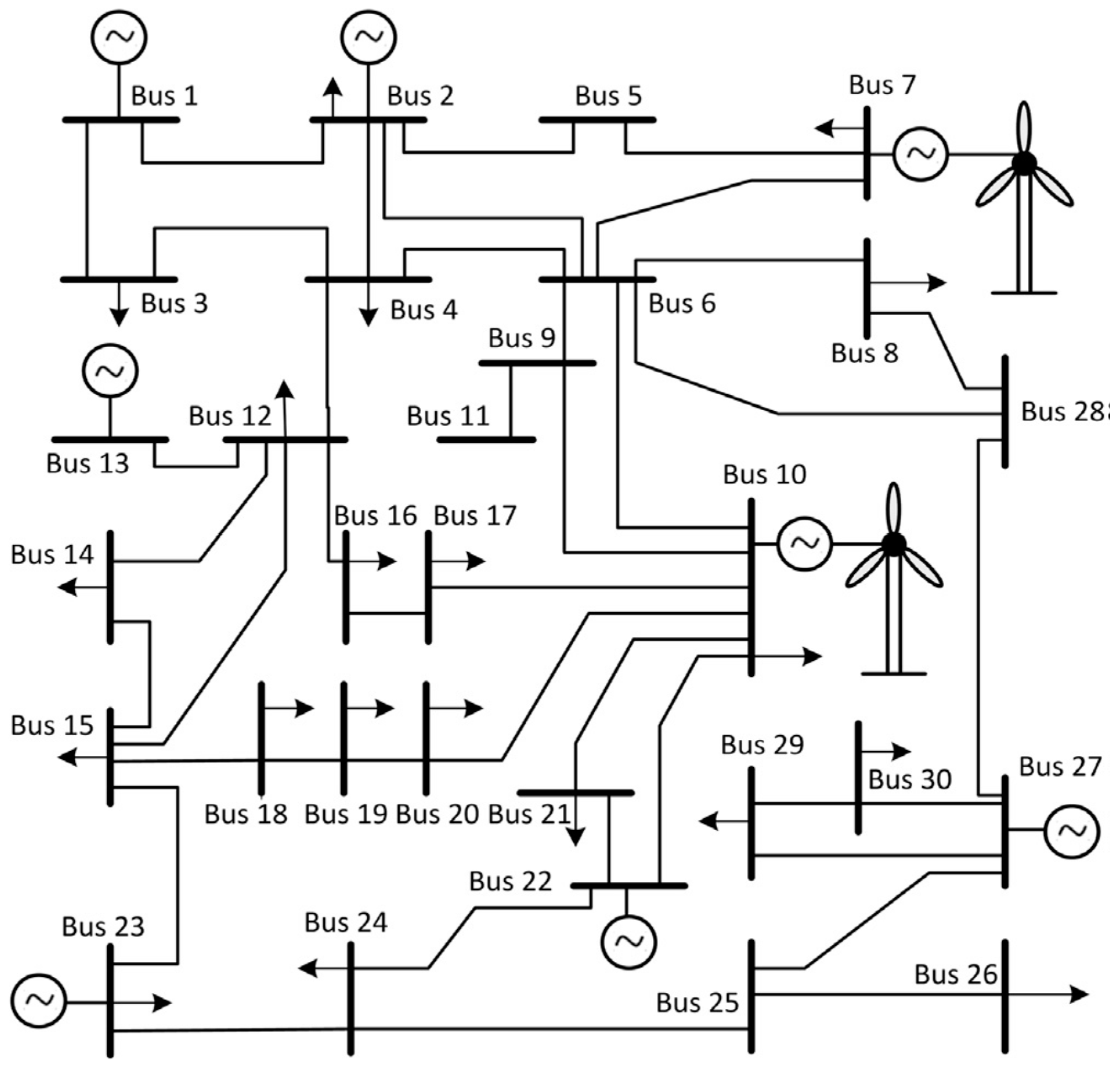
In this Section, by using Matlab R2014a software, our proposed approach is implemented on IEEE 30-bus test system [2, 6] with six NRGenCOs and 20 DisCOs. There are two additional wind farms connected to buses 7 and 10 [2], and the output power of the wind farms connected to bus 7 and 10 lies within the range of [0, 20] MW and [0, 30] MW, respectively. Figure 2 shows the schematic structure of the test system. Parameters of NRGenCOs’ and DisCOs’ bid functions are shown in Table 1 [6] and Table 2 [2], respectively.
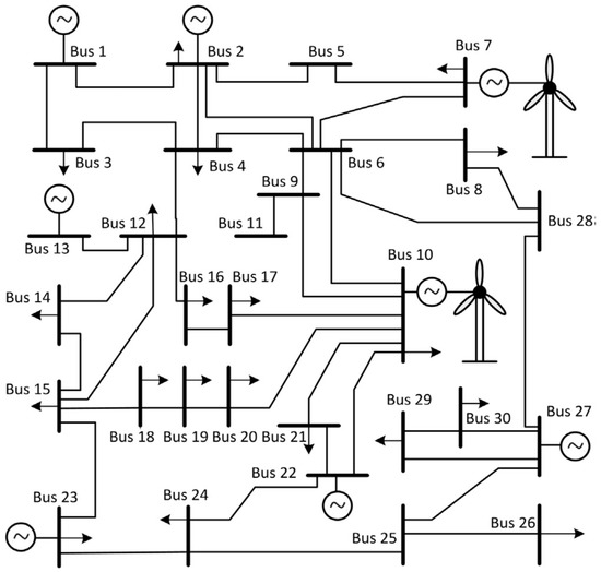
Figure 2.
Diagram of the test system. Note: For the sake of simplicity, here it is assumed that the maximum congestion constraint in all transmission lines is 25 MW.

Table 1.
Parameters of NRGenCOs’ bid functions.

Table 2.
Parameters of DisCOs’ bid functions.
In order to verify the superiority of our proposed method, the GDCAC-based method and the fuzzy Q-learning-based method [2] are implemented on this test system. There are three scenarios set in this paper for simulation and comparison.
In Scenario 1, every NRGenCO and DisCO searches for its optimal bidding strategy by using the GDCAC algorithm. In Scenario 2, NRGenCO1 searches for its optimal bidding strategy by using the fuzzy Q-learning algorithm, and other NRGenCOs and DisCOs using the GDCAC algorithm. In Scenario 3, every NRGenCO and DisCO searches for its optimal bidding strategy by using the fuzzy Q-learning algorithm.
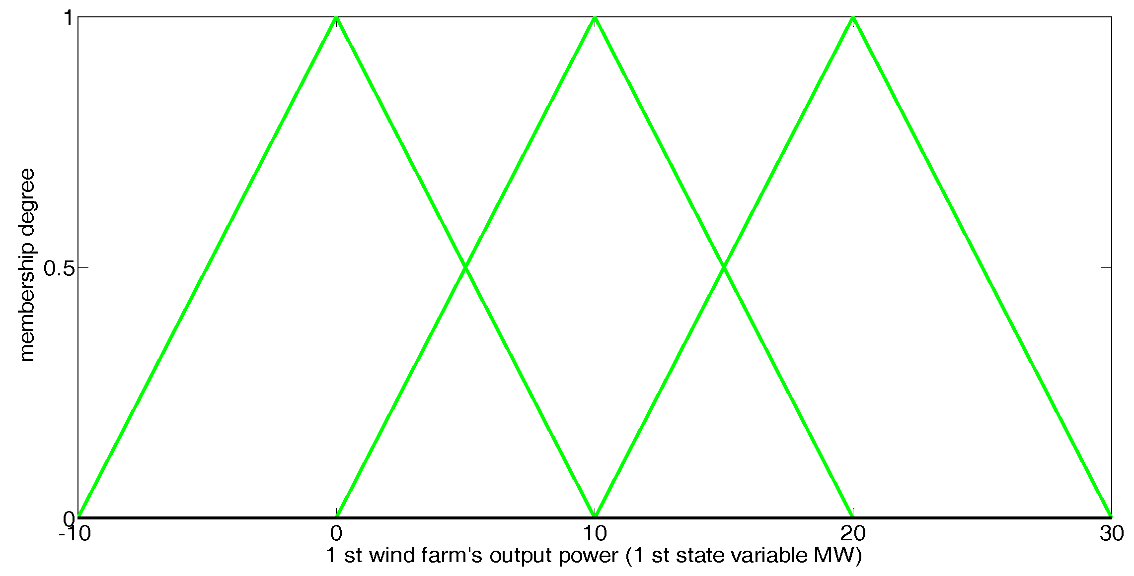
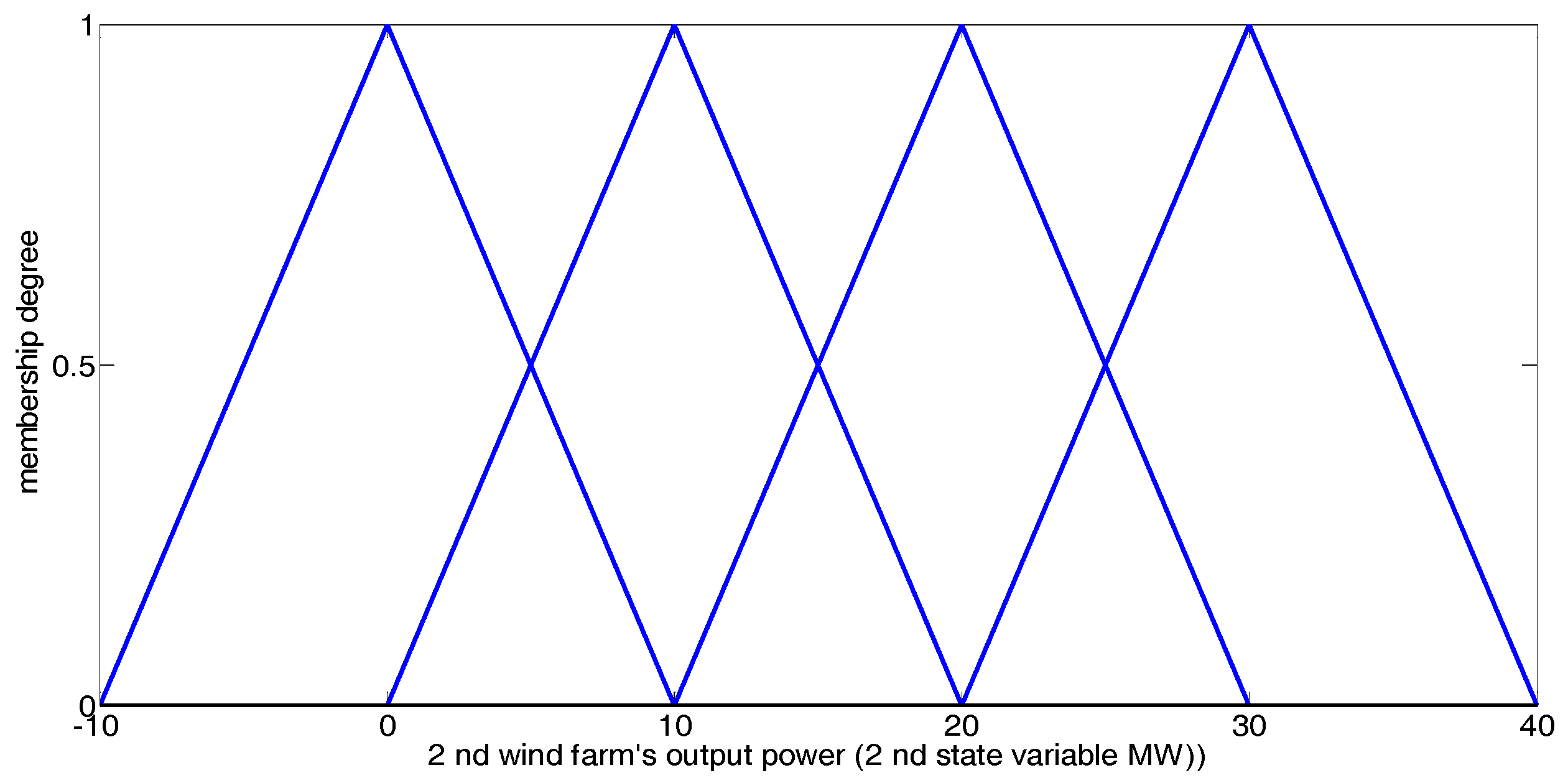
In our simulation, the output powers of the two wind farms together constitute the 2-dimensional state vector. Each fuzzy Q-learning-based agent (whose step-by-step learning procedure and method for fuzzy set definition can be found in [2]) defines three triangular fuzzy sets for the state variable 1, and 4 triangular fuzzy sets for state variable 2, as shown in Figure 3 and Figure 4. Table 3 presents the state and action sets of every NRGenCO and DisCO while taking Scenarios 1, 2, and 3 into consideration. The related parameters of the GDCAC algorithm and fuzzy Q-learning algorithm [2], which use the method to balance exploration and exploitation, are also listed in Table 3.
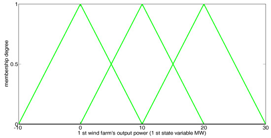
Figure 3.
Fuzzy sets for state variable 1 in fuzzy Q-learning-based EM model.
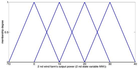
Figure 4.
Fuzzy sets for state variable 2 in the fuzzy Q-learning-based EM model.

Table 3.
Related information about the three scenarios.
In the Gauss radial basis function, we set the central point parameter matrix corresponding to state variable 1 and 2, which is expressed as follows:
5.2. Implementing a GDCAC-Based Approach on the Test System
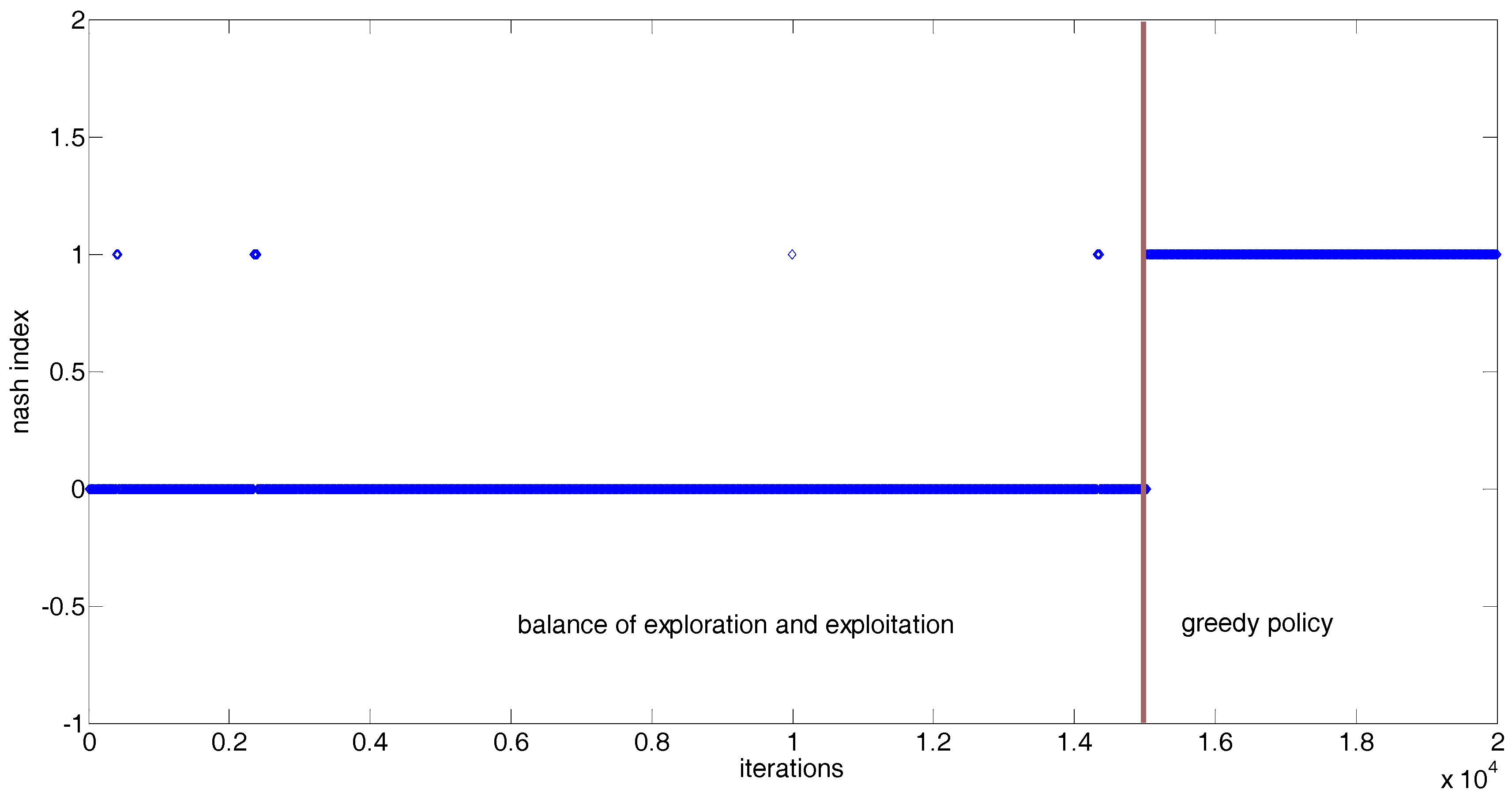
In this section, the feasibility of the GDCAC-based EM approach is studied by using Scenario 1, as proposed in Section 5.1. In our simulation in Scenario 1, 20,000 iterations are set for every NRGenCO and DisCO to bid in EM. Among the 20,000 iterations, the first 15,000 iterations (training iterations) are used to train every NRGenCO and DisCO to perceive the ability of distinguishing optimal bidding strategies under the exploration and exploitation policy; the last 5000 iterations (decision-making iterations) are used to help every NRGenCO and DisCO with decision-making under the greedy policy.
After 20,000 iterations of the bidding process, a Nash index is adopted in this paper to test whether the obtained bidding strategies of all NRGenCOs and DisCOs under any EM state reach Nash Equilibrium (NE) or not. Similar to the NE testing method in [2], the Nash index is equal to 1 when the NE under an EM state is reached and otherwise is equal to 0.
Because the EM state space is continuous, we cannot display the process of reaching NE under every given EM state in this paper. Figure 5 demonstrates the Nash indices obtained after each iteration in a case in which the state variables 1 and 2 are equal to 20 and 30 MW, respectively. From Figure 5, it can be seen that occurrences of NE during the first 15,000 iterations are very sparse, and the EM can reach NE during the last 5000 iterations. The reasons for this phenomenon are: (1) every NRGenCO and DisCO has not yet accumulated enough experience to make the optimal bidding decision during the first 15,000 iterations; (2) the exploration and exploitation policy may make every NRGenCO and DisCO choose sub-optimal bids during the first 15,000 iterations; (3) 15,000 iterations of the training process are enough for every NRGenCO and DisCO to perceive the ability of distinguishing optimal bidding strategies and to make the optimal bidding decision under greedy policy during the last 5000 iterations.
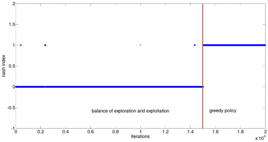
Figure 5.
Nash index during the learning iterations of the proposed GDCAC method when the state vector is (20, 30) MW.
When we make state variable 1 and 2 change randomly within interval [0, 20] MW and [0, 30] MW, respectively, in each iteration, the Nash indices obtained after 20000 iterations in 10 state samples are listed in Table 4.

Table 4.
Nash indices in 10 random state samples after 20,000 iterations.
From Table 4 it can be verified, to a certain extent, that the generalization ability of our proposed GDCAC-based EM approach can make the obtained strategies of all participants in face of any state point within the continuous space reach NE based on those finite and discrete sample state points occurred during the 20,000 iterations.
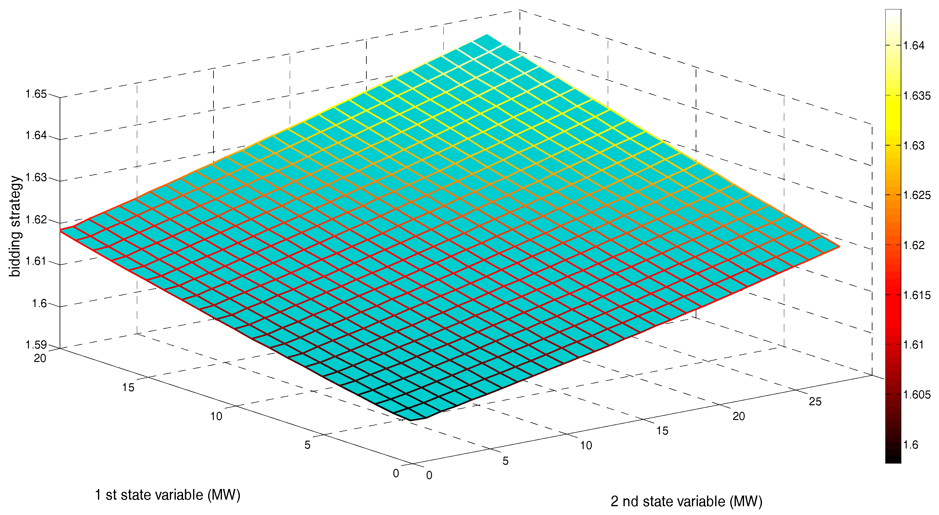
Figure 6 shows NRGenCO 2’s bidding strategy (kg2) in the face of any state point within after 20,000 iterations.

Figure 6.
Bidding strategy of NRGenCO2 corresponding to the state space after 15,000 training and 5000 decision-making iterations (considering transmission line congestion constraint).
From Figure 6, we can see that after 20,000 iterations, no matter the increase in the power output level of any one of the two wind farms, the value of NRGenCO2’s bidding strategy will increase accordingly. That is because increasing the power output levels of the two wind farms could cause congestion in the transmission lines connecting bus 1 to 2 and connecting bus 12 to 13, which limits the increase in NRGenCO2’s dispatched power output. Gradually, NRGenCO2, through repeatedly interacting with the EM environment over 20,000 iterations, learns that by increasing the value of its bidding strategy so as to maintain or increase the LMP level in bus 2, it could make comparatively more profit. Therefore, taking transmission congestion into account, some NRGenCOs’ market powers could be enhanced while increasing the wind power output.
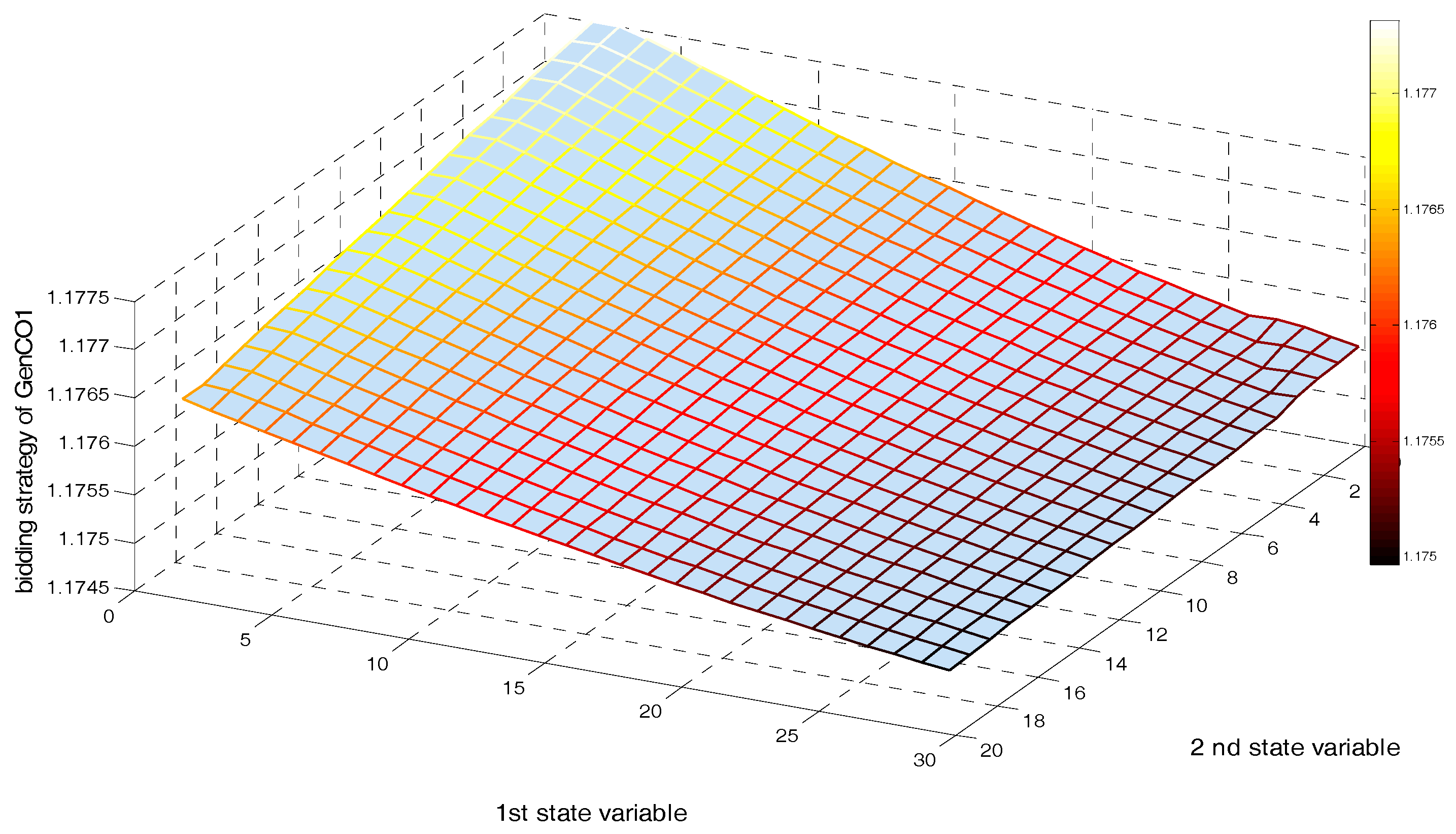
Figure 7 shows the NRGenCO2’s bidding strategy (kg2) corresponding to the state space after 20,000 iterations in the case of ignoring all transmission lines’ congestions in this test system. From Figure 7, we see that after 20,000 iterations, no matter the increase in the power output level of any one of the two wind farms, the value of NRGenCO2’s bidding strategy will decrease accordingly. In fact, other NRGenCOs’ bidding strategies are also subject to a similarly changing law. Therefore, if we ignore the transmission congestion in the test system, NRGenCOs’ market powers would be weakened while increasing the wind power output.
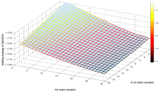
Figure 7.
Bidding strategy of NRGenCO2 corresponding to the state space after 15,000 training and 5000 decision-making iterations (ignoring transmission line congestion constraint).
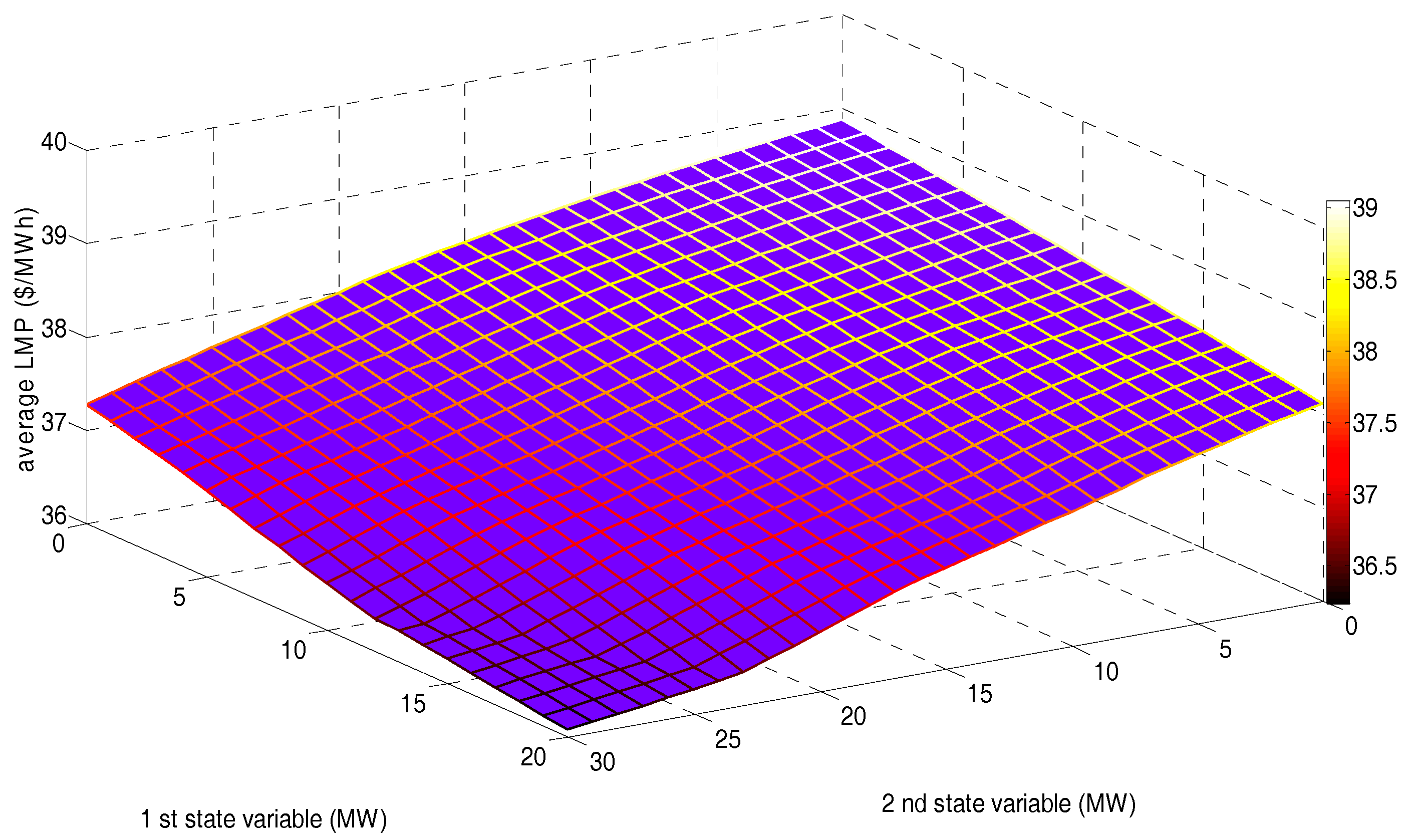
Figure 8 shows the average LMP of 30 buses (AVLMP) corresponding to the state space after 20,000 iterations.

Figure 8.
AVLMP corresponding to the state space after 15,000 training and 5000 decision-making iterations.
Figure 8 reveals that, although the market power of some NRGenCOs could be enhanced if the transmission capacities in some transmission lines were insufficient, the obtained AVLMP after 20,000 iterations decreases while increasing the wind power output level. We think there may be two main reasons for the phenomenon in Figure 8 that need to be further verified: (1) the marginal cost of the wind farm is significantly lower than that of all NRGenCOs (so we assume it is zero), which in turn pulls down the overall LMP level; (2) the increase in wind power output can reduce most agents’ market power and increase the degree of competition in the whole EM.
Figure 9 demonstrates the social welfare (SW) corresponding to the state space after 20,000 iterations. It is concluded from Figure 9 that increasing the wind power output level can not only pull down the overall LMP level, but also increase the overall SW.
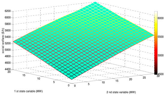
Figure 9.
Social welfare in state space after 15,000 training and 5000 decision-making iterations.
The computational formula of SW is as follows:
5.3. Comparative Study
From the perspective of economics, an effective EM modeling approach has two functions: to provide a bidding decision-making tool for every EM participant so as to increase its own profit in EM competition; and to enhance the economic efficiency of the whole market, e.g., by improving SW and reducing AVLMP. If we compare our proposed GDCAC-based EM approach with other approaches, the superiority of our proposed approach can be verified in two ways. When approaches adopted by other participants for bidding decision-making are fixed, a specific participant can get more profit with our proposed approach in market competition than with other approaches. In addition, with the increase in the number of participants applying our proposed approach as their bidding decision-making tool, SW in the market increases and AVLMP in the market decreases.
In [2], considering wind power penetration, it was verified that the fuzzy Q-learning-based hour-ahead EM modeling approach is superior to other approaches such as Q-learning, etc. in terms of improving SW and reducing AVLMP, etc.
In this section, a comparison between our proposed approach and the fuzzy Q-learning approach is carried out by implementing simulations on Scenarios 1, 2, and 3, respectively. The obtained simulation results of three scenarios after 20,000 iterations are studied and compared, which mainly contain all agents’ final profits, SWs and AVLMPs in those three scenarios (the ability to reach NE after enough iterations by applying the fuzzy Q-learning algorithm in EM modeling has been verified by [2]). In simulations on Scenarios 1, 2, and 3, we also make state variable 1 and 2 change randomly within interval [0 20] MW and [0 30] MW, respectively, in each iteration. Table 5, Table 6 and Table 7 demonstrate the obtained profit of every agent and the SW results of the three scenarios after 20,000 iterations in sample state (20, 30) MW, (10, 15) MW, and (4, 6) MW, respectively. The average AVLMP and SW of sample states in three scenarios after 20,000 iterations are demonstrated in Table 8, in which sample states constitute a discrete set as follows:
where (MW), (MW).

Table 5.
Profit of every agent and SW results of three scenarios in sample state (20, 30) MW.

Table 6.
Profit of every agent and SW results of three scenarios in sample state (10, 15) MW.

Table 7.
Profit of every agent and SW results of three scenarios in sample state (4, 6) MW.

Table 8.
Average AVLMP and SW results of sample states in the three scenarios.
- (1)
- No matter which of the three sample states, in Table 5, NRGenCO1’s final profit in Scenario 1 is 369.5193 ($/h), which is more than that in Scenario 2 (296.7915 ($/h)). In Table 6, NRGenCO1’s final profit in Scenario 1 is 484.2735 ($/h), which is more than that in Scenario 2 (408.0777 ($/h)). In Table 7, NRGenCO1’s final profit in Scenario 1 is 326.8942 ($/h), which is more than that in Scenario 2 (304.4191 ($/h)). Moreover, although we cannot compare NRGenCO1’s final profits in Scenarios 1 and 2 under every state point due to the continuous state space, the phenomenon that NRGenCO1’s final profit in Scenario 1 is more than its final profit in Scenario 2 can actually be found under every state point of the sample states in . As mentioned in Section 5.1, there is only one difference between Scenarios 1 and 2, which is that NRGenCO1 in Scenario 1 is a GDCAC-based agent that makes its bidding decisions based on our proposed GDCAC approach, while NRGenCO1 in Scenario 2 is a fuzzy Q-learning-based agent that makes its bidding decisions based on the fuzzy Q-learning approach. Therefore, it can, to some extent, be verified that a specific participant can get more profit with our proposed GDCAC approach in market competition than with the fuzzy Q-learning one proposed in [2].
- (2)
- No matter which of the three sample states, in Table 5, the order of final SWs in the three scenarios from high to low is Scenario 1 (6177.1 ($/h)), Scenario 2 (6108.2 ($/h)), and Scenario 3 (6063.4 ($/h)). In Table 6, the order of final SWs in the three scenarios from high to low is: Scenario 1 (5172.2 ($/h)), Scenario 2 (5123.6 ($/h)), and Scenario 3 (5102.5 ($/h)). In Table 7, the order of the final SWs in the three scenarios from high to low is: Scenario 1 (4639.1 ($/h)), Scenario 2 (4610.7 ($/h)), and Scenario 3 (4562.7 ($/h)). Moreover, although we cannot compare final SWs in Scenarios 1, 2 and 3 for every state point due to the continuous state space, the phenomenon that the order of the final SWs in the three scenarios from high to low are Scenario 1, Scenario 2, and Scenario 3 can actually be found under every state point of the sample states in . As mentioned in Section 5.1, every participant in Scenario 3 is a fuzzy Q-learning-based agent; NRGenCO1 in Scenario 2 is a fuzzy Q-learning-based agent while all the other participants in Scenario 2 are our proposed GDCAC-based ones, and every participant in Scenario 1 is our proposed GDCAC-based agent. Therefore, it can, to some extent, be verified that with the increase in the number of participants applying our proposed approach as their bidding decision-making tool, SW in the market increases.
From Table 8, it can be seen that:
- (1)
- The order of final average AVLMPs of sample states in the three scenarios, from low to high, is: Scenario 1 (37.0352 ($/MWh)), Scenario 2 (37.4531 ($/MWh)), and Scenario 3 (38.2237 ($/MWh)), which, to some extent, verifies the renewable power penetration in EM. The final average AVLMP of the sample states will be lowered by increasing the number of GDCAC-based agents.
- (2)
- The order of final average SWs of sample states in the three scenarios from high to low is: Scenario 1 (5329.5 ($/h)), Scenario 2 (5280.8 ($/h)), and Scenario 3 (5242.9 ($/h)), which, to some extent, verifies the renewable power penetration in EM. The final average SW of sample states will be increased by increasing the number of GDCAC-based agents.
- (3)
- Increasing SW as well as lowering clearing prices (represented by average AVLMPs) stands for the economic efficiency improvement in the whole market, which is proven, to some extent and through this comparative study, to be attributable to our proposed GDCAC approach.
Therefore, from the abovementioned analysis of Table 5, Table 6, Table 7 and Table 8, it is concluded that in bilateral hour-ahead EM with renewable power penetration, our proposed GDCAC approach is superior to the fuzzy Q-learning one from the perspective of economics. That is mainly because: (1) although both state spaces in the two EM modeling approaches are continuous, the action set of every agent in fuzzy Q-learning approach must be discrete, which is not the same as all continuous action spaces in the GDCAC approach; and (2) the phenomenon of discrete action sets makes it harder for an agent to obtain globally optimal actions.
Moreover, although it was verified in [2] that the fuzzy Q-learning approach is superior to the Q-learning one in EM modeling considering renewable power penetration, Table 9 still lists some simulation results obtained - from the GDCAC, fuzzy Q-learning, and Q-learning approaches after 20,000 iterations, respectively. In Table 9, simulation with the GDCAC approach is equivalent to simulation with Scenario 1, simulation with the fuzzy Q-learning approach is equivalent to simulation with Scenario 3, and simulation with Q-learning approach assumes every strategic participant in EM is the Q-learning-based agent with the same discrete action sets and relevant parameters as the fuzzy Q-learning approach (listed in Table 3) and with the same discrete state set as for the purpose of comparison.

Table 9.
The simulation results of the three approaches.
From Table 9, it can be seen that, from the perspective of economics, our proposed GDCAC approach is the most promising approach for EM modeling considering the renewable power penetration among the three approaches. The reason for low performance when applying Q-learning approach is due to both the discrete action and state sets within it. In addition, simulation with the Q-learning approach takes only about 3.1 min to reach a final result, which is the lowest among the three approaches. However, the time complexity of our proposed GDCAC approach (about 3.2 min) is also acceptable for hour-ahead EM modeling so that we can extend it to the modeling and simulation of more realistic and complex EM systems.
6. Conclusions
Bilateral spot EM is a more complicated type of EM in many countries in the world, where every player (GenCO and DisCO) chooses its bidding strategy within a continuous interval of values simultaneously in order to make more profit. Considering renewable resource penetration, the random fluctuation and continuous variation of renewable resource power generation make it more difficult to model the dynamic bidding process and the equilibrium in the bilateral spot EM. Since the GDCAC algorithm has been demonstrated to be an effective method in dealing with continuous state and action variables, in this paper we have proposed the application of a GDCAC algorithm for bilateral hour-ahead EM modeling considering renewable power penetration. The simulation results have verified the feasibility and scientific nature of our proposed approach, and some conclusions can be drawn as follows:
- (1)
- In our proposed GDCAC-based EM modeling approach, every agent needs no common knowledge about other agents’ costs or revenue functions, etc. and can make the decision to select an optimal bidding strategy within a continuous interval of values according to many renewable power generations randomly changing within a continuous state space, which can avoid the “Curse of Dimensionality”. The randomly fluctuating nature of renewable resource output does not affect the proposed EM approach’s ability to reach NE after enough iterations;
- (2)
- In our proposed GDCAC EM modeling approach, after enough iterations, although with the increase of renewable resource output some agents may have their bidding functions deviate more from their actual marginal cost or revenue functions because of congestions in some transmission lines, the overall SW still increases, which is the same as the conclusions drawn in [2];
- (3)
- Our proposed GDCAC EM modeling approach is superior to the fuzzy Q-learning approach (mentioned in [2]) in terms of increasing the profit of a specific agent and the overall SW and lowering the overall LMP level;
- (4)
- According to [40], the time complexity of GDCAC is O(n) (the relevant mathematical proof is proposed in [40]). However, when applying the GDCAC algorithm to EM modeling, because in every iteration we use the active set (AS) algorithm to solve the congestion management model for ISO, which needs 500 extra iterations, the time complexity of our proposed GDCAC-based EM modeling approach is O(500n). Nevertheless, our simulation with the proposed GDCAC-based EM modeling approach takes only about 3.2 min to reach the final result. That is to say, the time complexity of our GDCAC-based EM modeling approach is acceptable so that we can extend it to the modeling and simulation of more realistic and complex EM systems.
Moreover, our proposed approach can provide a bidding decision-making tool for participants to get more profit in EM with renewable power penetration. In addition, our proposed approach can provide an economic analysis tool for governments to design proper policies to promote the development of renewable resources.
Acknowledgments
This study was supported by the National Natural Science Foundation of China under Grant No. 71373076, the Fundamental Research Funds for the Central Universities under Grant No. JB2016183, and the Major State Research and Development Program of China under Grant Nos. 2016YFB0900500 and 2016YFB0900501.
Author Contributions
Huiru Zhao guided the research; Yuwei Wang established the model, implemented the simulation, and wrote this article; Mingrui Zhao collected references; Chuyu Sun and Qingkun Tan revised the language of this article.
Conflicts of Interest
The authors declare no conflict of interest.
References
- Alikhanzadeh, A.; Irving, M. Combined oligopoly and oligopsony bilateral electricity market model using CV equilibria. In Proceedings of the 2012 IEEE Power and Energy Society General Meeting, San Diego, CA, USA, 22–26 July 2012; pp. 1–8. [Google Scholar]
- Mohammad, R.S.; Salman, S. Application of fuzzy Q-learning for electricity market modeling by considering renewable power penetration. Renew. Sustain. Energy Rev. 2016, 56, 1172–1181. [Google Scholar]
- Aghaei, J.; Akbari, M.; Roosta, A.; Gitizadeh, M.; Niknam, T. Integrated renewable-conventional generation expansion planning using multi objective framework. IET Gener. Transm. Distrib. 2012, 6, 773–784. [Google Scholar] [CrossRef]
- Yu, N.; Liu, C.C.; Tesfatsion, L. Modeling of Suppliers' Learning Behaviors in an Electricity Market Environment. In Proceedings of the 2007 International Conference on Intelligent Systems, Niigata, Japan, 5–8 November 2007; pp. 1–6. [Google Scholar]
- Widén, J.; Carpman, N.; Castellucci, V.; Lingfors, D.; Olauson, J.; Remouit, F.; Bergkvist, M.; Grabbe, M.; Waters, R. Variability assessment and forecasting of renewables: A review for solar, wind, wave and tidal resources. Renew. Sustain. Energy Rev. 2015, 44, 356–375. [Google Scholar] [CrossRef]
- Buygi, M.O.; Zareipour, H.; Rosehart, W.D. Impacts of Large-Scale Integration of Intermittent Resources on Electricity Markets: A Supply Function Equilibrium Approach. IEEE Syst. J. 2012, 6, 220–232. [Google Scholar] [CrossRef]
- Al-Agtash, S.Y. Supply curve bidding of electricity in constrained power networks. Energy 2010, 35, 2886–2892. [Google Scholar] [CrossRef]
- Gao, F.; Sheble, G.B.; Hedman, K.W.; Yu, C.-N. Optimal bidding strategy for GENCOs based on parametric linear programming considering incomplete information. Int. J. Electr. Power Energy Syst. 2015, 66, 272–279. [Google Scholar] [CrossRef]
- Borghetti, A.; Massucco, S.; Silvestro, F. Influence of feasibility constrains on the bidding strategy selection in a day-ahead electricity market session. Electr. Power Syst. Res. 2009, 79, 1727–1737. [Google Scholar] [CrossRef]
- Kumar, J.V.; Kumar, D.M.V. Generation bidding strategy in a pool based electricity market using Shuffled Frog Leaping Algorithm. Appl. Soft Comput. 2014, 21, 407–414. [Google Scholar] [CrossRef]
- Wang, J.; Zhou, Z.; Botterud, A. An evolutionary game approach to analyzing bidding strategies in electricity markets with elastic demand. Energy 2011, 36, 3459–3467. [Google Scholar] [CrossRef]
- Min, C.G.; Kim, M.K.; Park, J.K.; Yoon, Y.T. Game-theory-based generation maintenance scheduling in electricity markets. Energy 2013, 55, 310–318. [Google Scholar] [CrossRef]
- Shivaie, M.; Ameli, M.T. An environmental/techno-economic approach for bidding strategy in security-constrained electricity markets by a bi-level harmony search algorithm. Renew. Energy 2015, 83, 881–896. [Google Scholar] [CrossRef]
- Ladjici, A.A.; Tiguercha, A.; Boudour, M. Equilibrium Calculation in Electricity Market Modeled as a Two-stage Stochastic Game using competitive Coevolutionary Algorithms. IFAC Proc. Vol. 2012, 45, 524–529. [Google Scholar] [CrossRef]
- Su, W.; Huang, A.Q. A game theoretic framework for a next-generation retail electricity market with high penetration of distributed residential electricity suppliers. Appl. Energy 2014, 119, 341–350. [Google Scholar] [CrossRef]
- Rahimiyan, M.; Mashhadi, H.R. Supplier’s optimal bidding strategy in electricity pay-as-bid auction: Comparison of the Q-learning and a model-based approach. Electr. Power Syst. Res. 2008, 78, 165–175. [Google Scholar] [CrossRef]
- Ziogos, N.P.; Tellidou, A.C. An agent-based FTR auction simulator. Electr. Power Syst. Res. 2011, 81, 1239–1246. [Google Scholar] [CrossRef]
- Santos, G.; Fernandes, R.; Pinto, T.; Praa, I.; Vale, Z.; Morais, H. MASCEM: EPEX SPOT Day-Ahead market integration and simulation. In Proceedings of the 2015 18th International Conference on Intelligent System Application to Power Systems (ISAP), Porto, Portugal, 11–16 September 2015; pp. 1–5. [Google Scholar]
- Liu, Z.; Yan, J.; Shi, Y.; Zhu, K.; Pu, G. Multi-agent based experimental analysis on bidding mechanism in electricity auction markets. Int. J. Electr. Power Energy Syst. 2012, 43, 696–702. [Google Scholar] [CrossRef]
- Li, H.; Tesfatsion, L. The AMES wholesale power market test bed: A computational laboratory for research, teaching, and training. In Proceedings of the 2009 IEEE Power & Energy Society General Meeting, Calgary, AB, Canada, 26–30 July 2009; pp. 1–8. [Google Scholar]
- Conzelmann, G.; Boyd, G.; Koritarov, V.; Veselka, T. Multi-agent power market simulation using EMCAS. In Proceedings of the IEEE Power Engineering Society General Meeting, San Francisco, CA, USA, 12–16 June 2005; Volume 3, pp. 2829–2834. [Google Scholar]
- Sueyoshi, T. An agent-based approach equipped with game theory: Strategic collaboration among learning agents during a dynamic market change in the California electricity crisis. Energy Econ. 2010, 32, 1009–1024. [Google Scholar] [CrossRef]
- Mahvi, M.; Ardehali, M.M. Optimal bidding strategy in a competitive electricity market based on agent-based approach and numerical sensitivity analysis. Energy 2011, 36, 6367–6374. [Google Scholar] [CrossRef]
- Zhao, H.; Wang, Y.; Guo, S.; Zhao, M.; Zhang, C. Application of gradient descent continuous actor-critic algorithm for double-side day-ahead electricity market modeling. Energies 2016, 9, 725. [Google Scholar] [CrossRef]
- Lau, A.Y.F.; Srinivasan, D.; Reindl, T. A reinforcement learning algorithm developed to model GenCo strategic bidding behavior in multidimensional and continuous state and action spaces. In Proceedings of the 2013 IEEE Symposium on Adaptive Dynamic Programming and Reinforcement Learning (ADPRL), Singapore, 16–19 April 2013; pp. 116–123. [Google Scholar]
- Sharma, K.C.; Bhakar, R.; Tiwari, H.P. Strategic bidding for wind power producers in electricity markets. Energy Convers. Manag. 2014, 86, 259–267. [Google Scholar]
- Vilim, M.; Botterud, A. Wind power bidding in electricity markets with high wind penetration. Appl. Energy 2014, 118, 141–155. [Google Scholar] [CrossRef]
- Kang, C.; Du, E.; Zhang, N.; Chen, Q.; Huang, H.; Wu, S. Renewable energy trading in electricity market: Review and prospect. South. Power Syst. Technol. 2016, 10, 16–23. [Google Scholar]
- Dallinger, D.; Wietschel, M. Grid integration of intermittent renewable energy sources using price-responsive plug-in electric vehicles. Renew. Sustain. Energy Rev. 2012, 16, 3370–3382. [Google Scholar] [CrossRef]
- Shafie-khah, M.; Moghaddam, M.P.; Sheikh-El-Eslami, M.K. Development of a virtual power market model to investigate strategic and collusive behavior of market players. Energy Policy 2013, 61, 717–728. [Google Scholar] [CrossRef]
- Reeg, M.; Hauser, W.; Wassermann, S.; Weimer-Jehle, W. AMIRIS: An Agent-Based Simulation Model for the Analysis of Different Support Schemes and Their Effects on Actors Involved in the Integration of Renewable Energies into Energy Markets. In Proceedings of the 2012 23rd International Workshop on Database and Expert Systems Applications, Vienna, Austria, 3–7 September 2012; pp. 339–344. [Google Scholar]
- Haring, T.; Andersson, G.; Lygeros, J. Evaluating market designs in power systems with high wind penetration. In Proceedings of the 2012 9th International Conference on the European Energy Market (EEM), Florence, Italy, 10–12 May 2012; pp. 1–8. [Google Scholar]
- Soares, T.; Santos, G.; Pinto, T.; Morais, H.; Pinson, P.; Vale, Z. Analysis of strategic wind power participation in energy market using MASCEM simulator. In Proceedings of the 2015 18th International Conference on Intelligent System Application to Power Systems (ISAP), Porto, Portugal, 11–16 September 2015; pp. 1–6. [Google Scholar]
- Abrell, J.; Kunz, F. Integrating Intermittent Renewable Wind Generation-A Stochastic Multi-Market Electricity Model for the European Electricity Market. Netw. Spat. Econ. 2015, 15, 117–147. [Google Scholar] [CrossRef]
- Zhao, Q.; Shen, Y.; Li, M. Control and Bidding Strategy for Virtual Power Plants with Renewable Generation and Inelastic Demand in Electricity Markets. IEEE Trans. Sustain. Energy 2016, 7, 562–575. [Google Scholar] [CrossRef]
- Zou, P.; Chen, Q.; Xia, Q.; Kang, C.; He, G.; Chen, X. Modeling and algorithm to find the economic equilibrium for pool-based electricity market with the changing generation mix. In Proceedings of the 2015 IEEE Power & Energy Society General Meeting, Denver, CO, USA, 26–30 July 2015; pp. 1–5. [Google Scholar]
- Ela, E.; Milligan, M.; Bloom, A.; Botterud, A.; Townsend, A.; Levin, T.; Frew, B.A. Wholesale electricity market design with increasing levels of renewable generation: Incentivizing flexibility in system operations. Electr. J. 2016, 29, 51–60. [Google Scholar] [CrossRef]
- Liuhui, W.; Xian, W.; Shanghua, Z. Electricity market equilibrium analysis for strategic bidding of wind power producer with demand response resource. In Proceedings of the 2016 IEEE PES Asia-Pacific Power and Energy Engineering Conference, Xi’an, China, 25–28 October 2016; pp. 181–185. [Google Scholar]
- Green, R.; Vasilakos, N. Market behaviour with large amounts of intermittent generation. Energy Policy 2010, 38, 3211–3220. [Google Scholar] [CrossRef]
- Chen, G. Research on Value Function Approximation Methods in Reinforcement Learning. Master’s Thesis, Soochow University, Suzhou, China, 2014. [Google Scholar]
- Chen, Z. Study on Locational Marginal Prices and Congestion Management Algorithm. Ph.D. Thesis, North China Electric Power University, Beijing, China, 2007. [Google Scholar]
© 2017 by the authors. Licensee MDPI, Basel, Switzerland. This article is an open access article distributed under the terms and conditions of the Creative Commons Attribution (CC BY) license (http://creativecommons.org/licenses/by/4.0/).


