Article

Coupled Least Squares Identification Algorithms for Multivariate Output-Error Systems

Key Laboratory of Advanced Process Control for Light Industry (Ministry of Education), Jiangnan University, Wuxi 214122, China
*
Author to whom correspondence should be addressed.
Algorithms 2017, 10(1), 12; https://doi.org/10.3390/a10010012
Submission received: 17 November 2016 / Revised: 5 January 2017 / Accepted: 6 January 2017 / Published: 12 January 2017

Abstract

:
This paper focuses on the recursive identification problems for a multivariate output-error system. By decomposing the system into several subsystems and by forming a coupled relationship between the parameter estimation vectors of the subsystems, two coupled auxiliary model based recursive least squares (RLS) algorithms are presented. Moreover, in contrast to the auxiliary model based recursive least squares algorithm, the proposed algorithms provide a reference to improve the identification accuracy of the multivariate output-error system. The simulation results confirm the effectiveness of the proposed algorithms.

1. Introduction

Multivariable systems are popular in industrial processes [1,2,3] and a number of successful methods have been developed to solve the identification and control problems of multivariable systems [4,5,6,7]. For example, Zhang and Hoagg used a candidate-pool approach to identify the feedback and feedforward transfer function matrices and presented a frequency-domain technique for identifying multivariable feedback and feedforward systems [8]; Salhi and Kamoun proposed a recursive algorithm to estimate the parameters of the dynamic linear part and the static nonlinear part of multivariable Hammerstein systems [9].
The idea of the auxiliary model is to use the measurable information to construct a dynamical model and to replace the unknown variables in the information vector with the output of the auxiliary model [10,11]. There are two typical identification methods for multivariate output-error systems: stochastic gradient (SG) algorithms [12,13] and the recursive least squares (RLS) algorithms [14,15]. The SG algorithm requires lower computational cost, but the RLS algorithm has a faster convergence rate than the SG algorithm [16]. The RLS algorithm has been applied to the identification of various systems [17,18]. For example, on the basis of the work in [19], Jin et al. proposed an auxiliary model based recursive least squares algorithm for autoregressive output-error autoregressive systems [20]; and Wang and Tang presented an auxiliary model based recursive least squares algorithm for a class of linear-in-parameter output-error moving average systems [21].
Although the RLS algorithm can be applied to identify the parameter of the multivariate output-error systems, it requires computing the matrix inversion (see Remark 1 in the following section), resulting in a large computational burden [22]. This motivates us to study a new coupled least squares algorithm without involving matrix inversion. The coupling identification concept is useful for simplifying the parameter estimation of the coupled parameter multivariable systems [23]. It is based on the coupled relationship of the parameter estimates between the subsystems of a multivariable system [24,25,26]. The purpose of the coupling identification is to reduce the redundant estimation of the subsystem parameter vectors and to avoid computing the matrix inversion of the RLS algorithm. Recently, a coupled least squares algorithm has been proposed for multiple linear regression systems [22].
This paper focuses on the parameter estimation of multivariate output-error systems, and the main contributions of this paper are the following:
  • for multivariate output-error systems, this paper derives two coupled least squares parameter estimation algorithms by using the auxiliary model identification idea and the coupling identification concept;
  • the proposed algorithms can generate more accurate parameter estimates, and avoid computing the matrix inversion in the multivariable RLS algorithm, for the purpose of reducing computational load.
The rest of this paper is organized as follows: Section 2 gives some definitions and the identification model of multivariate output-error systems. Section 3 presents two new coupled auxiliary model identification algorithms. Section 4 gives two simulation examples to validate the effectiveness of the proposed methods. Finally, some concluding remarks are offered in Section 5.

2. System Description and Identification Model

Let us introduce some notation. The symbol I m is an m × m identity matrix; 1 n is an n-dimensional column vector whose elements are 1; the superscript T denotes the matrix transpose; the norm of the matrix X is defined as X 2 : = tr [ X X T ] ; the symbol ⊗ denotes the Kronecker product or the direct product: if A = [ a i j ] R m × n , B = [ b i j ] R p × q , then A B = [ a i j B ] R m p × n q ; col [ X ] denotes the vector formed by the column of the matrix X, that is, if X : = [ x 1 , x 2 , , x n ] R m × n , then col [ X ] = [ x 1 T , x 2 T , , x n T ] T R m n . X ^ ( t ) denotes the estimate of X at time t and X ˜ ( t ) : = X ^ ( t ) X denotes the estimation error.
Consider the following multivariate output-error system:
y ( t ) = x ( t ) + v ( t ) ,
x ( t ) : = Φ s ( t ) θ A ( z ) R m ,
A ( z ) : = 1 + a 1 z 1 + a 2 z 2 + + a n a z n a R ,
where y ( t ) : = [ y 1 ( t ) , y 2 ( t ) , , y m ( t ) ] T R m is the system output vector and the noisy measurement of x ( t ) , Φ s ( t ) R m × n is the information matrix consisting of the input–output data, θ R n is the parameter vector, and v ( t ) : = [ v 1 ( t ) , v 2 ( t ) , , v m ( t ) ] T R m is the observation noise vector with zero mean, and z 1 is a unit backward shift operator with [ z 1 y ( t ) = y ( t 1 ) ] .
Assume that the degrees m, n, n a are known and when t 0 , y ( t ) = 0 , Φ s ( t ) = 0 and v ( t ) = 0 . { Φ s ( t ) , y ( t ) } is the available measurement data.
Equations (1) and (2) can be expressed as
x ( t ) = Φ x ( t ) a + Φ s ( t ) θ ,
y ( t ) = Φ ( t ) ϑ + v ( t ) , Φ x ( t ) : = [ x ( t 1 ) , x ( t 2 ) , , x ( t n a ) ] R m × n a , Φ ( t ) : = [ Φ x ( t ) , Φ s ( t ) ] R m × n 0 , a : = [ a 1 , a 2 , , a n a ] T R n a , ϑ : = a θ R n 0 , n 0 : = n a + n .
Let ϑ ^ ( t ) : = [ a ^ T ( t ) , θ ^ T ( t ) ] R n 0 be the estimate of ϑ at time t.
For the identification model in (5), Φ x ( t ) is the information matrix that consists of the unknown inner variables x ( t j ) ’s, so we construct an auxiliary model x a ( t ) , and define the estimate of Φ x ( t ) as
Φ ^ x ( t ) : = [ x a ( t 1 ) , x a ( t 2 ) , , x a ( t n a ) ] R m × n a .
Then, we use Φ ^ x ( t ) and Φ s ( t ) to construct the estimate of Φ ( t ) as
Φ ^ ( t ) : = [ Φ ^ x ( t ) , Φ s ( t ) ] R m × n 0 .
Thus, according to (4), we can obtain the auxiliary model,
x a ( t ) = Φ ^ x ( t ) a ^ ( t ) + Φ s ( t ) θ ^ ( t ) = Φ ^ ( t ) ϑ ^ ( t ) .
The objective of this paper is to use the auxiliary model identification idea and the coupling identification concept to derive new methods for estimating the system parameters θ , a 1 , a 2 , , a n a from the observation data { y ( t ) , Φ s ( t ) } and to confirm the theoretical results with simulation examples.

3. The Multivariate Auxiliary Model Coupled Identification Algorithm

3.1. The Auxiliary Model Based Recursive Least Squares Algorithm

According to the identification model in (5), define a cost function:
J 1 ( ϑ ) : = j = 1 t y ( j ) Φ ( j ) ϑ 2 .
Based on the auxiliary model identification idea and on the derivation of the RLS algorithm [27,28], we use the output x a ( t ) as the unknown inner vector x ( t ) and replace the unknown information matrix Φ ( t ) with its estimate Φ ^ ( t ) , and obtain the following auxiliary model based recursive least squares (AM-RLS) algorithm:
ϑ ^ ( t ) = ϑ ^ ( t 1 ) + L ( t ) [ y ( t ) Φ ^ ( t ) ϑ ^ ( t 1 ) ] ,
L ( t ) = P ( t 1 ) Φ ^ T ( t ) [ I m + Φ ^ ( t ) P ( t 1 ) Φ ^ T ( t ) ] 1 ,
P ( t ) = P ( t 1 ) L ( t ) Φ ^ ( t ) P ( t 1 ) ,
Φ ^ ( t ) = [ Φ ^ x ( t ) , Φ s ( t ) ] ,
Φ ^ x ( t ) = [ x a ( t 1 ) , x a ( t 2 ) , , x a ( t n a ) ] ,
x a ( t ) = Φ ^ ( t ) ϑ ^ ( t ) .
The steps of computing the parameter estimation vector ϑ ^ ( t ) by the AM-RLS algorithm are listed in the following:
  • Set the initial values: t = 1 , ϑ ^ ( 0 ) = 1 n 0 / p 0 , P ( 0 ) = p 0 I n 0 , x a ( t j ) = 1 m / p 0 , j = 1 , 2, ⋯, n a , p 0 = 10 6 . Set the data length L.
  • Collect the observation data { Φ s ( t ) , y ( t ) } and form the information matrix Φ ^ x ( t ) by (10).
  • Form Φ ^ ( t ) by (9), and compute L ( t ) by (7) and P ( t ) by (8).
  • Update the parameter estimation vector ϑ ^ ( t ) by (6).
  • Compute the output x a ( t ) of the auxiliary model using (11).
  • If t = L , stop the recursive computation and obtain the parameter estimates; otherwise, increase t by 1 and go to Step 2.
Remark 1.
For the multivariable RLS algorithm in (6)–(10), we can see from (7) that it requires computing the matrix inversion [ I m + Φ ^ ( t ) P ( t 1 ) Φ ^ T ( t ) ] 1 R m × m at each step, resulting in heavy computational load, especially for large m (the number of outputs). This is the drawback of the multivariable RLS algorithm in (6)–(10). This motivates us to study new coupled parameter identification methods.

3.2. The Coupled Subsystem Auxiliary Model Based Recursive Least Squares Algorithm

The coupling identification is usually used to reduce the redundant estimates of the system parameter vectors, based on the coupled relationship of the parameter estimates between subsystems [22].
Let ϕ i T ( t ) R 1 × n 0 be the ith row of the information matrix Φ ( t ) , i.e.,
Φ ( t ) : = ϕ 1 T ( t ) ϕ 2 T ( t ) ϕ m T ( t ) R m × n 0 .
From (5), we obtain m identification models (subsystems)
y i ( t ) = ϕ i T ( t ) ϑ + v i ( t ) , i = 1 , 2 , , m .
From here, all subsystems contain a common parameter vector ϑ R n 0 . In general, one of the subsystems can be used to identify the parameter vector ϑ ; however, in order to improve the parameter estimation precision, we should make full use of the information in all subsystems for identifying ϑ .
Based on the RLS algorithm in (6)–(11), and applying the auxiliary model idea, we replace the unknown variables ϕ i ( t ) in the identification algorithm with their estimates ϕ ^ i ( t ) , and obtain m RLS algorithms from (13), namely, the subsystem recursive least squares (S-RLS) algorithm,
ϑ ^ i ( t ) = ϑ ^ i ( t 1 ) + L i ( t ) [ y i ( t ) ϕ ^ i T ( t ) ϑ ^ i ( t 1 ) ] , ϑ ^ i ( 0 ) = 1 n 0 / p 0 ,
L i ( t ) = P i ( t ) ϕ ^ i ( t ) = P i ( t 1 ) ϕ ^ i ( t ) [ 1 + ϕ ^ i T ( t ) P i ( t 1 ) ϕ ^ i ( t ) ] 1 ,
P i ( t ) = [ I n 0 L i ( t ) ϕ ^ i T ( t ) ] P i ( t 1 ) , P i ( 0 ) = p 0 I n 0 , i = 1 , 2 , , m .
From here, we can see that there is no coupled relationship between the subsystem parameter estimation vector ϑ ^ i ( t ) .
Remark 2.
For i = 1 , 2 , , m , we can obtain m estimation vectors ϑ ^ i ( t ) from (14)–(16), and they are all the estimates of the common parameter vector ϑ in all subsystems, resulting in a large amount of redundant parameter estimates. One way is to use their average as the estimate of ϑ , that is
ϑ ^ ( t ) : = ϑ ^ 1 ( t ) + ϑ ^ 2 ( t ) + + ϑ ^ m ( t ) m R n 0 .
If we regard the parameter estimate ϑ ^ ( t ) in (17) as the output parameter vector, then each S-RLS identification algorithm is still independent. According to the coupling identification concept, we use ϑ ^ ( t 1 ) to replace ϑ ^ i ( t 1 ) in the S-RLS algorithm, and get the coupled subsystem AM-RLS (C-S-AM-RLS) algorithm:
ϑ ^ i ( t ) = ϑ ^ ( t 1 ) + L i ( t ) [ y i ( t ) ϕ ^ i T ( t ) ϑ ^ ( t 1 ) ] ,
L i ( t ) = P i ( t ) ϕ ^ i ( t ) = P i ( t 1 ) ϕ ^ i ( t ) [ 1 + ϕ ^ i T ( t ) P i ( t 1 ) ϕ ^ i ( t ) ] 1 ,
P i ( t ) = [ I n 0 L i ( t ) ϕ ^ i T ( t ) ] P i ( t 1 ) , i = 1 , 2 , , m ,
ϑ ^ ( t ) = ϑ ^ 1 ( t ) + ϑ ^ 2 ( t ) + + ϑ ^ m ( t ) m ,
Φ ^ x ( t ) = [ x a ( t 1 ) , x a ( t 2 ) , , x a ( t n a ) ] ,
Φ ^ ( t ) = [ Φ ^ x ( t ) , Φ s ( t ) ]
= [ ϕ ^ 1 ( t ) , ϕ ^ 2 ( t ) , , ϕ ^ m ( t ) ] T ,
x a ( t ) = Φ ^ ( t ) ϑ ^ ( t ) .
The steps of computing the parameter estimation vector ϑ ^ ( t ) by the C-S-AM-RLS algorithm in (18)–(25) are listed in the following:
  • Set the initial values: t = 1 , ϑ ^ ( 0 ) = 1 n 0 / p 0 , P i ( 0 ) = p 0 I n 0 , x a ( t j ) = 1 m / p 0 , j = 1 , 2, ⋯, n a , p 0 = 10 6 . Set the data length L.
  • Collect the observation data { Φ s ( t ) , y ( t ) } and form the information matrix Φ ^ x ( t ) by (22).
  • Form Φ ^ ( t ) by (23) and read ϕ ^ i ( t ) from Φ ^ ( t ) in (24).
  • For each i, i = 1 , 2 , , m , compute L i ( t ) by (19), and P i ( t ) by (20), and update the parameter estimation vector ϑ ^ i ( t ) by (18).
  • Compute ϑ ^ ( t ) by (21) and x a ( t ) by (25).
  • If t = L , stop the recursive computation and obtain the parameter estimates; otherwise, increase t by 1 and go to Step 2.
Remark 3.
The C-S-AM-RLS algorithm in (18)–(25) uses the estimate ϑ ^ ( t 1 ) on the right-hand side of (18) instead of ϑ ^ i ( t 1 ) on the right-hand side of (14) for i = 1 , 2 , , m . Thus, the C-S-AM-RLS algorithm is different from the S-RLS algorithm.

3.3. The Coupled Auxiliary Model Based Recursive Least Squares Algorithm

In order to avoid the redundant parameter estimates, we use the coupling identification concept to derive a coupled AM-RLS algorithm based on the C-S-AM-RLS algorithm.
Referring to the partially coupled SG identification method [24], and with the help of the Jacobi or Gauss–Seidel iterative algorithm, replacing ϑ ^ m ( t 1 ) with ϑ ^ 1 ( t 1 ) for i = 1 , replacing ϑ ^ i ( t 1 ) with ϑ ^ i 1 ( t ) for i = 2 , 3 , , m , we can obtain the following coupled auxiliary model based recursive least squares (C-AM-RLS) identification algorithm:
ϑ ^ 1 ( t ) = ϑ ^ m ( t 1 ) + L 1 ( t ) [ y 1 ( t ) ϕ ^ 1 T ( t ) ϑ ^ m ( t 1 ) ] ,
L 1 ( t ) = P m ( t 1 ) ϕ ^ 1 ( t ) [ 1 + ϕ ^ 1 T ( t ) P m ( t 1 ) ϕ ^ 1 ( t ) ] 1 ,
P 1 ( t ) = [ I n 0 L 1 ( t ) ϕ ^ 1 T ( t ) ] P m ( t 1 ) ,
ϑ ^ i ( t ) = ϑ ^ i 1 ( t ) + L i ( t ) [ y i ( t ) ϕ ^ i T ( t ) ϑ ^ i 1 ( t ) ] ,
L i ( t ) = P i 1 ( t ) ϕ ^ i ( t ) [ 1 + ϕ ^ i T ( t ) P i 1 ( t ) ϕ ^ i ( t ) ] 1 ,
P i ( t ) = [ I n 0 L i ( t ) ϕ ^ i T ( t ) ] P i 1 ( t ) , i = 2 , 3 , , m ,
Φ ^ x ( t ) = [ x a ( t 1 ) , x a ( t 2 ) , , x a ( t n a ) ] ,
Φ ^ ( t ) = [ Φ ^ x ( t ) , Φ s ( t ) ]
= [ ϕ ^ 1 ( t ) , ϕ ^ 2 ( t ) , , ϕ ^ m ( t ) ] T ,
x a ( t ) = Φ ^ ( t ) ϑ ^ ( t ) .
In the above algorithm in (26)–(35), ϑ ^ i ( t ) R n 0 is the parameter estimation vector of the ith subsystem at time t, L i ( t ) R n 0 is the gain vector of the ith subsystem at time t, P i ( t ) R n 0 × n 0 is the covariance matrix of the ith subsystem at time t. ϑ ^ i 1 ( t ) and P i 1 ( t ) are the parameter estimation vector and the covariance matrix of the ( i 1 ) th subsystem at time t, respectively; ϑ ^ m ( t 1 ) and P m ( t 1 ) are the parameter estimation vector and the covariance matrix of the mth subsystem at time t 1 , respectively, the system parameter estimation vector is defined by the parameter estimation vector of the mth subsystem at time t: ϑ ^ ( t ) = ϑ ^ m ( t ) .
The procedure of computing the parameter estimation vector ϑ ^ m ( t ) in (26)–(35) is as follows.
  • Set the initial values: t = 1 , θ ^ m ( 0 ) = 1 n 0 / p 0 , P m ( 0 ) = p 0 I n 0 , x a ( t j ) = 1 m / p 0 , j = 1 , 2, ⋯, n a , p 0 = 10 6 . Set the data length L.
  • Collect the observation data y ( t ) and Φ s ( t ) , and construct Φ ^ x ( t ) and Φ ^ ( t ) by (32) and (33).
  • Read ϕ ^ i ( t ) from Φ ^ ( t ) in (34), compute L 1 ( t ) and P 1 ( t ) by (27) and (28), and update the parameter estimation vector ϑ ^ 1 ( t ) by (26).
  • For i = 2 , 3 , , m , compute L i ( t ) and P i ( t ) by (30) and (31), and update the parameter estimation vector ϑ ^ i ( t ) by (29).
  • Obtain the parameter estimation vector ϑ ^ ( t ) = ϑ ^ m ( t ) and compute x a ( t ) by (35).
  • If t = L , stop the recursive computation and obtain the parameter estimates; otherwise, increase t by 1 and go to Step 2.
Remark 4.
The C-AM-RLS algorithm in (26)–(35) uses the estimate ϑ ^ i 1 ( t ) on the right-hand side of (29) instead of ϑ ^ i ( t 1 ) on the right-hand side of (14) for i = 2 , 3 , , m . When computing ϑ ^ 1 ( t ) , the C-AM-RLS algorithm uses the estimate ϑ ^ m ( t 1 ) on the right-hand side of (26) instead of ϑ ^ i ( t 1 ) on the right-hand side of (14) with i = 1 . Thus, the C-AM-RLS algorithm is different from the S-RLS algorithm.

4. Examples

Example 1.
Consider the following multivariate output-error system:
y ( t ) = Φ s ( t ) θ A ( z ) + v ( t ) , Φ s ( t ) = y 1 ( t 2 ) u 2 ( t 2 ) y 1 ( t 2 ) sin ( t / π ) u 1 ( t 1 ) + u 2 ( t 2 ) u 2 ( t 1 ) sin ( u 2 ( t 2 ) ) y 1 ( t 2 ) sin ( y 2 ( t 2 ) ) y 2 ( t 2 ) u 1 ( t 2 ) u 1 ( t 2 ) u 2 ( t 2 ) u 2 ( t 1 ) cos ( t / π ) , θ = [ θ 1 , θ 2 , θ 3 , θ 4 ] T = [ 0.25 , 0.47 , 0.50 , 0.57 ] T R 4 , A ( z ) = 1 + a 1 z 1 + a 2 z 2 = 1 + 0.30 z 1 + 0.64 z 2 , ϑ = [ a 1 , a 2 , θ 1 , θ 2 , θ 3 , θ 4 ] T = [ 0.30 , 0.64 , 0.25 , 0.47 , 0.50 , 0.57 ] T R 6 .
In simulation, we generate two persistent excitation signal sequences with zero mean and unit variances as the inputs { u 1 ( t ) } and { u 2 ( t ) } , and take v 1 ( t ) and v 2 ( t ) to be two white noise sequences with zero mean and variances σ 1 2 for v 1 ( t ) , and σ 2 2 for v 2 ( t ) . Taking σ 1 2 = σ 2 2 = σ 2 = 0.50 2 , the data length L = 3000, and applying the AM-RLS, C-S-AM-RLS and C-AM-RLS algorithms to estimate the parameters of this system, respectively, the parameter estimates are shown in Table 1, Table 2 and Table 3, and the estimation errors δ : = θ ^ ( t ) θ / θ versus t are shown in Figure 1 and Figure 2.
From Table 1, Table 2 and Table 3 and Figure 1 and Figure 2, we can draw the following conclusions.
  • The parameter estimation errors by the presented algorithms become smaller and smaller and go to zero with the increasing of time t.
  • In contrast to the AM-RLS algorithm, the proposed C-S-AM-RLS and C-AM-RLS algorithms have faster convergence rates and more accurate parameter estimates with the same simulation conditions.
Example 2.
Consider the following 2-input 2-output system:
y ( t ) = Q ( z ) A ( z ) u ( t ) + v ( t ) , A ( z ) = 1 + a 1 z 1 + a 2 z 2 = 1 0.19 z 1 0.15 z 2 , Q ( z ) = Q 1 z 1 + Q 2 z 2 = 0.31 0.25 0.28 0.23 z 1 + 0.65 0.38 0.41 0.62 z 2 , a = [ a 1 , a 2 ] T = [ 0.19 , 0.15 ] T R 2 , θ T = [ Q 1 , Q 2 ] = 0.31 0.25 0.65 0.38 0.28 0.23 0.41 0.62 R 2 × 4 .
This example system can be transformed into the multivariate output-error system:
y ( t ) = Φ s ( t ) θ A ( z ) + v ( t ) , φ ( t ) = [ u T ( t 1 ) , u T ( t 2 ) ] T R 4 , Φ s ( t ) = I 2 φ T ( t ) = u 1 ( t 1 ) u 2 ( t 1 ) u 1 ( t 2 ) u 2 ( t 2 ) 0 0 0 0 0 0 0 0 u 1 ( t 1 ) u 2 ( t 1 ) u 1 ( t 2 ) u 2 ( t 2 ) R 2 × 8 , Φ ^ ( t ) = x 1 ( t 1 ) x 1 ( t 2 ) u 1 ( t 1 ) u 2 ( t 1 ) u 1 ( t 2 ) x 2 ( t 1 ) x 2 ( t 2 ) 0 0 0 u 2 ( t 2 ) 0 0 0 0 0 u 1 ( t 1 ) u 2 ( t 1 ) u 1 ( t 2 ) u 2 ( t 2 ) R 2 × 10 , ϑ = [ a T , col [ θ ] T ] T = [ a 1 , a 2 , θ 1 , θ 2 , θ 3 , θ 4 , θ 5 , θ 6 , θ 7 , θ 8 ] T = [ 0.19 , 0.15 , 0.31 , 0.25 , 0.65 , 0.38 , 0.28 , 0.23 , 0.41 , 0.62 ] T R 10 .
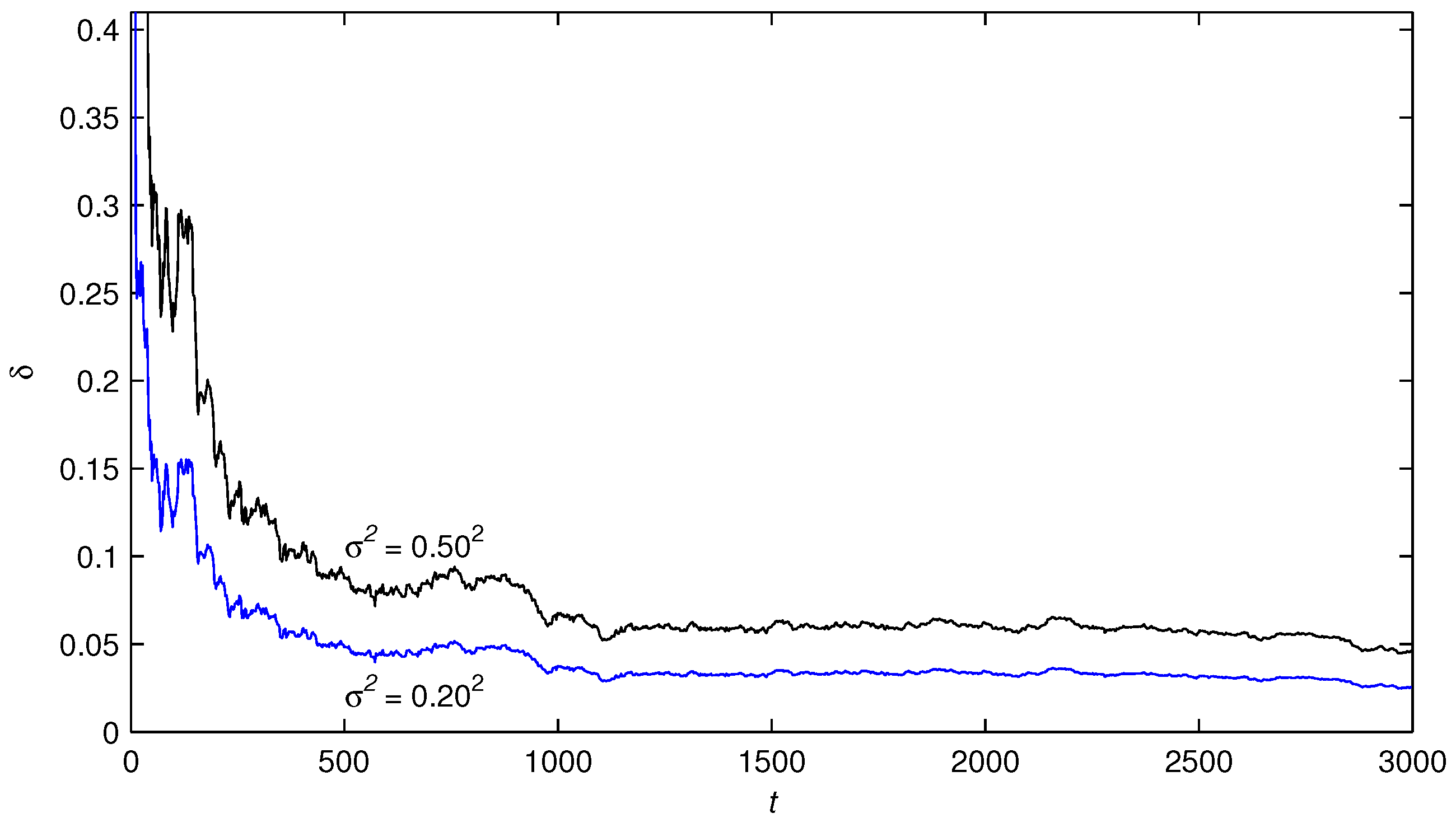
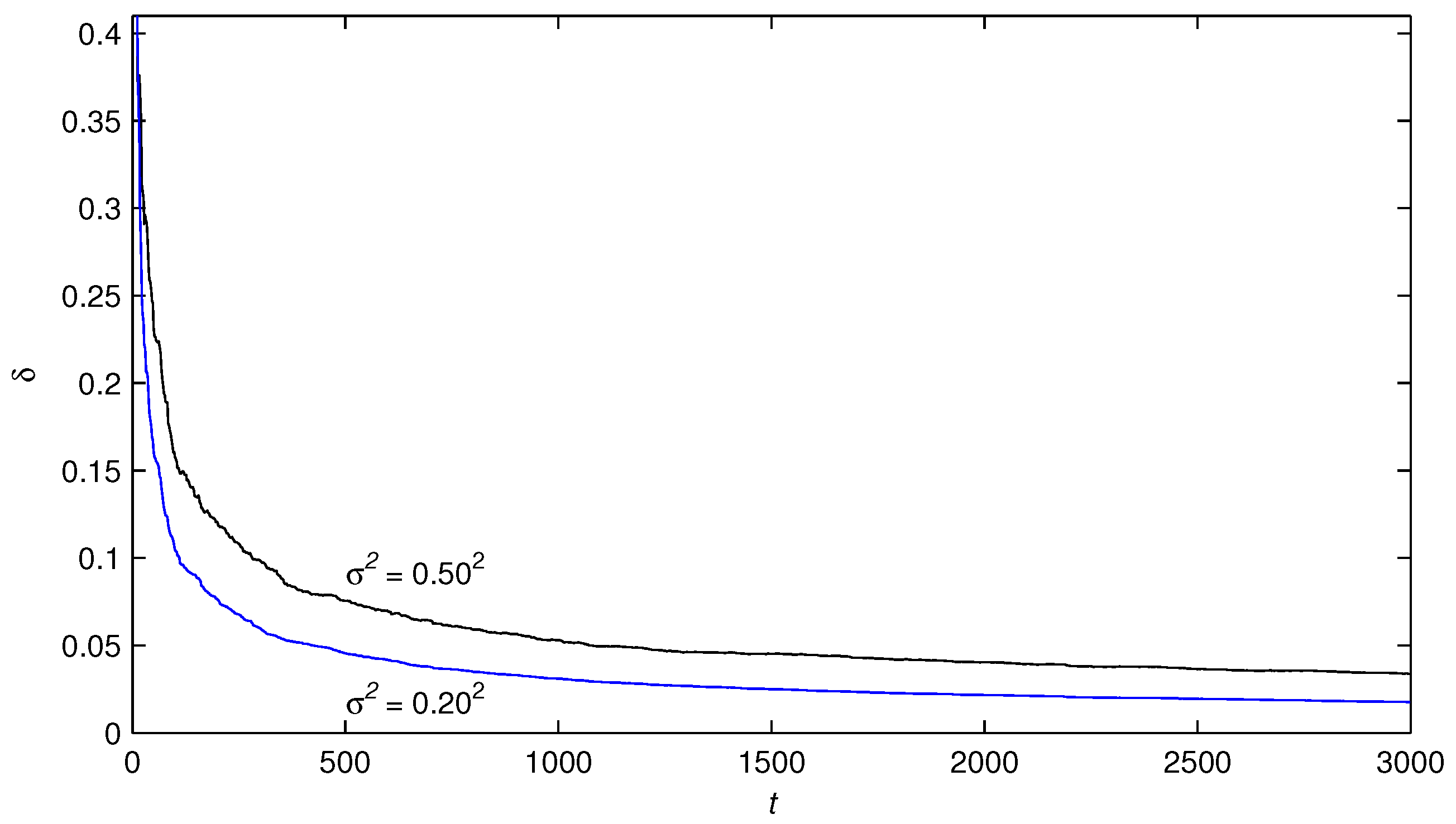
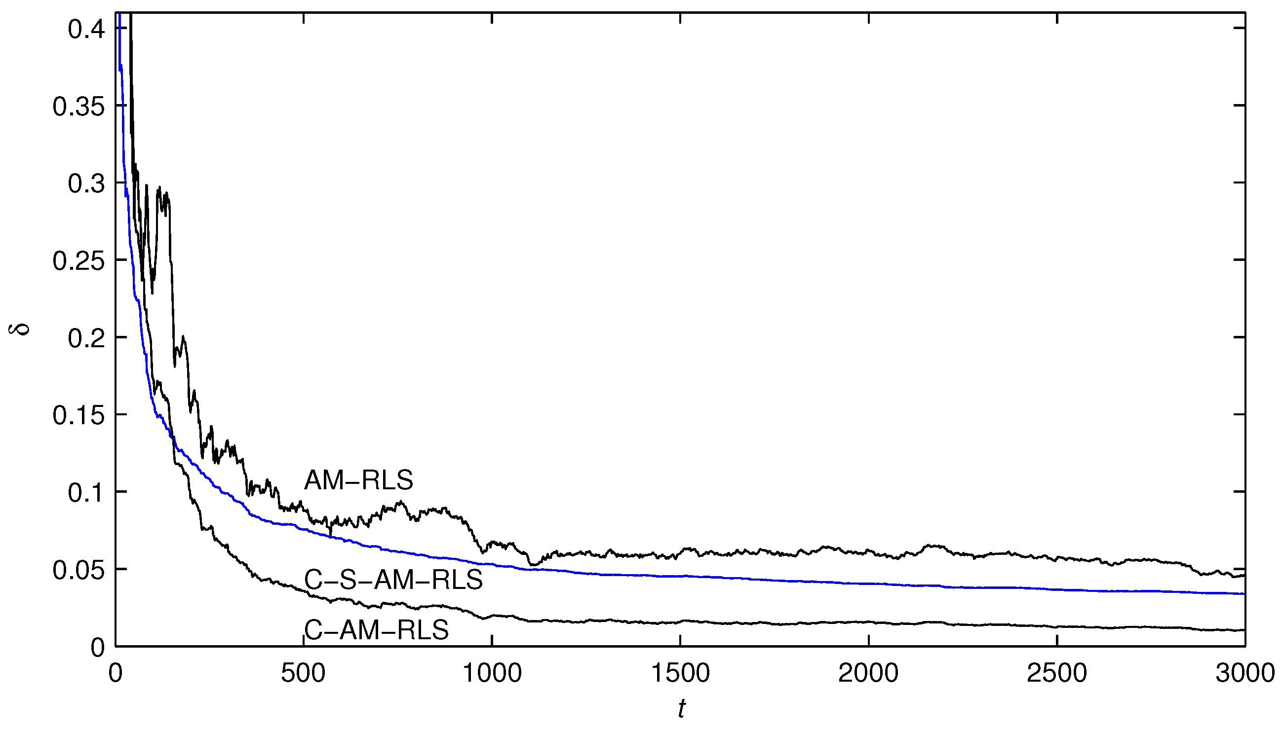
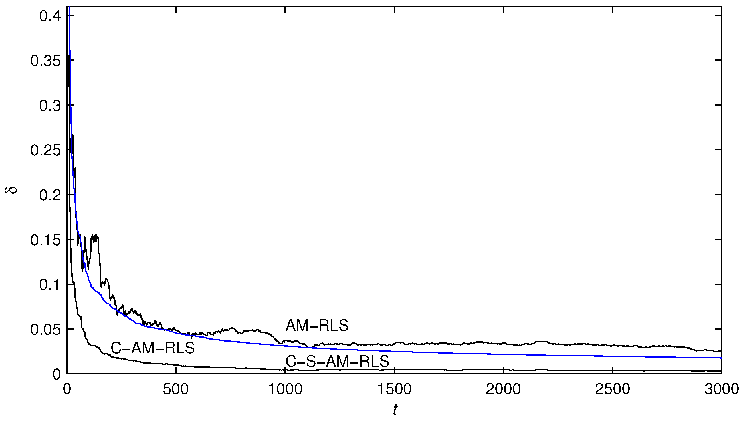
The simulation conditions are similar to those of Example 1. Applying the AM-RLS algorithm, the C-S-AM-RLS algorithm and the C-AM-RLS algorithm with σ 2 = 0.50 2 and σ 2 = 0.20 2 to estimate the parameters of this system, respectively, the parameter estimates are shown in Table 4, Table 5 and Table 6, and the estimation errors δ versus t are shown in Figure 3, Figure 4, Figure 5, Figure 6 and Figure 7.
From Table 4, Table 5 and Table 6 and Figure 3, Figure 4, Figure 5, Figure 6 and Figure 7, we can draw the following conclusions:
  • In contrast to the AM-RLS algorithm, the proposed C-S-AM-RLS and C-AM-RLS algorithms have faster convergence rates and more accurate parameter estimates with the same simulation conditions, and the C-AM-RLS algorithm can obtain the most accurate estimates for the system parameters.
  • The parameter estimation errors given by the proposed algorithms are smaller under a lower noise level—see Table 4, Table 5 and Table 6 and Figure 3, Figure 4, Figure 5, Figure 6 and Figure 7.

5. Conclusions

By means of the auxiliary model identification idea, this paper employs the coupling identification concept to propose a novel recursive identification method for multivariate output-error systems. The proposed methods have the following properties:
  • The C-S-AM-RLS algorithm and the C-AM-RLS algorithm are presented by forming a coupled relationship between the parameter estimation vectors of the subsystems, and they avoid computing the matrix inversion in the multivariable AM-RLS algorithm so they require lower computational load and achieve highly accurate parameter estimates.
  • With the noise-to-signal ratios decreasing, the parameter estimation errors given by the proposed algorithms become smaller.
The basic idea of the proposed algorithms in this paper can be extended and applied to other fields [29,30,31].

Acknowledgments

This work was supported in part by the National Natural Science Foundation of China (No. 61293194) and and Natural Science Research of Colleges and Universities in Jiangsu Province (No. 16KJB120007, China).

Author Contributions

Feng Ding conceived the whole paper and supervised his student Wu Huang to write the paper and Wu Huang designed and performed the simulation experiments. Both authors have read and approved the final manuscript.

Conflicts of Interest

The authors declare no conflict of interest.

References

  1. Ding, F. System Identification—New Theory and Methods; Science Press: Beijing, China, 2013. [Google Scholar]
  2. Ding, F. System Identification—Performances Analysis for Identification Methods; Science Press: Beijing, China, 2014. [Google Scholar]
  3. Ding, F. System Identification—Multi-Innovation Identification Theory and Methods; Science Press: Beijing, China, 2016. [Google Scholar]
  4. Liu, Y.J.; Tao, T.Y. A CS recovery algorithm for model and time delay identification of MISO-FIR systems. Algorithms 2015, 8, 743–753. [Google Scholar] [CrossRef]
  5. Ding, J.L. Data filtering based recursive and iterative least squares algorithms for parameter estimation of multi-input output systems. Algorithms 2016, 9. [Google Scholar] [CrossRef]
  6. Tsubakino, D.; Krstic, M.; Oliveira, T.R. Exact predictor feedbacks for multi-input LTI systems with distinct input delays. Automatica 2016, 71, 143–150. [Google Scholar] [CrossRef]
  7. Tian, Y.; Jin, Q.W.; Lavery, J.E. 1 Major component detection and analysis (1 MCDA): Foundations in two dimensions. Algorithms 2013, 6, 12–28. [Google Scholar] [CrossRef]
  8. Zhang, X.Y.; Hoagg, J.B. Subsystem identification of multivariable feedback and feedforward systems. Automatica 2016, 72, 131–137. [Google Scholar] [CrossRef]
  9. Salhi, H.; Kamoun, S. A recursive parametric estimation algorithm of multivariable nonlinear systems described by Hammerstein mathematical models. Appl. Math. Model. 2015, 39, 4951–4962. [Google Scholar] [CrossRef]
  10. Wang, Y.J.; Ding, F. Novel data filtering based parameter identification for multiple-input multiple-output systems using the auxiliary model. Automatica 2016, 71, 308–313. [Google Scholar] [CrossRef]
  11. Zhang, Y.; Zhao, Z.; Cui, G.M. Auxiliary model method for transfer function estimation from noisy input and output data. Appl. Math. Model. 2015, 39, 4257–4265. [Google Scholar] [CrossRef]
  12. Li, P.; Feng, J.; de Lamare, R.C. Robust rank reduction algorithm with iterative parameter optimization and vector perturbation. Algorithms 2015, 8, 573–589. [Google Scholar] [CrossRef]
  13. Filipovic, V.Z. Consistency of the robust recursive Hammerstein model identification algorithm. J. Frankl. Inst. 2015, 352, 1932–1945. [Google Scholar] [CrossRef]
  14. Guo, L.J.; Wang, Y.J.; Wang, C. A recursive least squares algorithm for pseudo-linear arma systems using the auxiliary model and the filtering technique. Circuits Syst. Signal Process. 2016, 35, 2655–2667. [Google Scholar] [CrossRef]
  15. Meng, D.D.; Ding, F. Model equivalence-based identification algorithm for equation-error systems with colored noise. Algorithms 2015, 8, 280–291. [Google Scholar] [CrossRef]
  16. Wang, D.Q.; Zhang, W. Improved least squares identification algorithm for multivariable Hammerstein systems. J. Frankl. Inst. 2015, 352, 5292–5307. [Google Scholar] [CrossRef]
  17. Wu, C.Y.; Tsai, J.S.H.; Guo, S.M. A novel on-line observer/Kalman filter identification method and its application to input-constrained active fault-tolerant tracker design for unknown stochastic systems. J. Frankl. Inst. 2015, 352, 1119–1151. [Google Scholar] [CrossRef]
  18. Bako, L. Adaptive identification of linear systems subject to gross errors. Automatica 2016, 67, 192–199. [Google Scholar] [CrossRef]
  19. Ding, F.; Liu, G.; Liu, X.P. Parameter estimation with scarce measurements. Automatica 2011, 47, 1646–1655. [Google Scholar] [CrossRef]
  20. Jin, Q.B.; Wang, Z.; Liu, X.P. Auxiliary model-based interval-varying multi-innovation least squares identification for multivariable OE-like systems with scarce measurements. J. Process Control 2015, 35, 154–168. [Google Scholar] [CrossRef]
  21. Wang, C.; Tang, T. Recursive least squares estimation algorithm applied to a class of linear-in-parameters output-error moving average systems. Appl. Math. Lett. 2014, 29, 36–41. [Google Scholar] [CrossRef]
  22. Ding, F. Coupled-least-squares identification for multivariable systems. IET Control Theory Appl. 2013, 7, 68–79. [Google Scholar] [CrossRef]
  23. Radenkovic, M.; Tadi, M. Self-tuning average consensus in complex networks. J. Frankl. Inst. 2015, 352, 1152–1168. [Google Scholar] [CrossRef]
  24. Ding, F.; Liu, G.; Liu, X.P. Partially coupled stochastic gradient identification methods for non-uniformly sampled systems. IEEE Trans. Autom. Control 2010, 55, 1976–1981. [Google Scholar] [CrossRef]
  25. Eldem, V.; Şahan, G. The effect of coupling conditions on the stability of bimodal systems in R3. Syst. Control Lett. 2016, 96, 141–150. [Google Scholar] [CrossRef]
  26. Wu, K.N.; Tian, T.; Wang, L.M. Synchronization for a class of coupled linear partial differential systems via boundary control. J. Frankl. Inst. 2016, 353, 4062–4073. [Google Scholar] [CrossRef]
  27. Meng, D.D. Recursive least squares and multi-innovation gradient estimation algorithms for bilinear stochastic systems. Circuits Syst. Signal Process. 2016, 35. [Google Scholar] [CrossRef]
  28. Wang, Y.J.; Ding, F. The filtering based iterative identification for multivariable systems. IET Control Theory Appl. 2016, 10, 894–902. [Google Scholar] [CrossRef]
  29. Wang, T.Z.; Qi, J.; Xu, H. Fault diagnosis method based on FFT-RPCA-SVM for cascaded-multilevel inverter. ISA Trans. 2016, 60, 156–163. [Google Scholar] [CrossRef] [PubMed]
  30. Wang, T.Z.; Wu, H.; Ni, M.Q. An adaptive confidence limit for periodic non-steady conditions fault detection. Mech. Syst. Signal Process. 2016, 72–73, 328–345. [Google Scholar] [CrossRef]
  31. Feng, L.; Wu, M.H.; Li, Q.X. Array factor forming for image reconstruction of one-dimensional nonuniform aperture synthesis radiometers. IEEE Geosci. Remote Sens. Lett. 2016, 13, 237–241. [Google Scholar] [CrossRef]
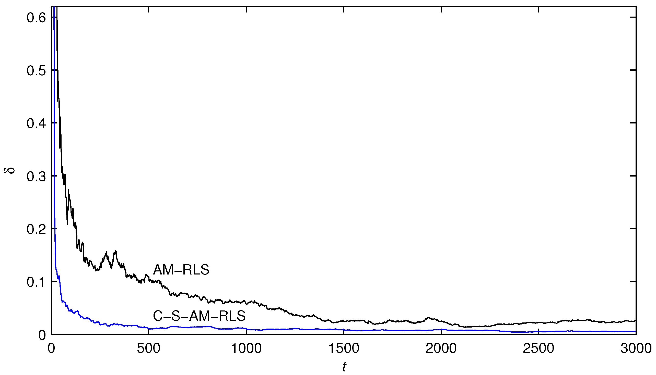
Figure 1. The AM-RLS and the C-S-AM-RLS estimation errors δ versus t for Example 1.
Algorithms 10 00012 g001
Figure 2. The AM-RLS and the C-AM-RLS estimation errors δ versus t for Example 1.
Algorithms 10 00012 g002
Figure 3. The AM-RLS estimation errors δ versus t with different σ 2 for Example 2.
Algorithms 10 00012 g003
Figure 4. The C-S-AM-RLS estimation errors δ versus t with different σ 2 for Example 2.
Algorithms 10 00012 g004
Figure 5. The C-AM-RLS estimation errors δ versus t with different σ 2 for Example 2.
Algorithms 10 00012 g005
Figure 6. The AM-RLS, C-S-AM-RLS and C-AM-RLS estimation errors δ versus t for Example 2 ( σ 2 = 0.50 2 ).
Algorithms 10 00012 g006
Figure 7. The AM-RLS, C-S-AM-RLS and C-AM-RLS estimation errors δ versus t for Example 2 ( σ 2 = 0.20 2 ).
Algorithms 10 00012 g007
Table 1. The AM-RLS estimates and their errors for Example 1.
t a 1 a 2 θ 1 θ 2 θ 3 θ 4 δ ( % )
1000.191690.46405−0.299210.51505−0.690030.5614724.77137
2000.241290.55426−0.263620.52514−0.610300.5600913.91359
5000.243610.55706−0.243610.47651−0.569450.5329410.96959
10000.298570.61286−0.246540.45360−0.559280.571975.78088
20000.311470.64219−0.233710.47639−0.518220.579772.53112
30000.317430.65208−0.234050.47050−0.489510.558192.65000
True values0.300000.64000−0.250000.47000−0.500000.57000
Table 2. The C-S-AM-RLS estimates and their errors for Example 1.
t a 1 a 2 θ 1 θ 2 θ 3 θ 4 δ ( % )
1000.290970.63357−0.272540.45781−0.497000.526484.44497
2000.297600.62737−0.263540.45916−0.502410.547352.69357
5000.296890.63747−0.252170.46685−0.505390.559601.11229
10000.298870.63910−0.251960.46698−0.502830.558261.08848
20000.301510.63810−0.249350.46850−0.500980.559610.92996
30000.303130.63900−0.246470.46872−0.503020.566430.58689
True values0.300000.64000−0.250000.47000−0.500000.57000
Table 3. The C-AM-RLS estimates and their errors for Example 1.
t a 1 a 2 θ 1 θ 2 θ 3 θ 4 δ ( % )
1000.290050.63637−0.256150.45607−0.492310.584832.14162
2000.296230.64525−0.251400.46821−0.503670.571510.67931
5000.296860.63477−0.255120.47214−0.501080.561531.01842
10000.302660.64036−0.247820.46668−0.502680.571150.48179
20000.300910.64021−0.247400.46931−0.501160.570560.26815
30000.302020.64160−0.248310.46919−0.498230.568210.34814
True values0.300000.64000−0.250000.47000−0.500000.57000
Table 4. The AM-RLS estimates and errors with different noise variances for Example 2.
σt a 1 a 2 θ 1 θ 2 θ 3 θ 4 θ 5 θ 6 θ 7 θ 8 δ ( % )
0.50100−0.07767−0.05531−0.366620.249560.48032−0.312060.31519−0.062570.417470.6239424.42046
200−0.12975−0.19484−0.392700.195520.54739−0.398010.25127−0.152920.408690.5986915.11250
500−0.19310−0.17229−0.366090.209230.61180−0.375650.30089−0.224500.471330.604448.75946
1000−0.19356−0.18464−0.350770.269290.61180−0.400970.29274−0.240580.417680.584576.77306
2000−0.16577−0.16642−0.355100.265880.63592−0.381380.27095−0.246430.432110.582396.17573
3000−0.17437−0.15862−0.349550.261430.63990−0.381570.26516−0.241550.418200.594854.64800
0.20100−0.14504−0.09948−0.341080.249260.56565−0.344260.29779−0.135840.409470.6250112.55557
200−0.16080−0.17384−0.356530.219840.59626−0.389550.26341−0.186630.407290.607838.16496
500−0.19361−0.16177−0.341300.227320.62940−0.377720.29134−0.226860.443720.611914.82443
1000−0.19260−0.16915−0.332760.260750.62898−0.391650.28698−0.235810.414170.600503.75051
2000−0.17637−0.15883−0.335130.258800.64247−0.380680.27492−0.239110.422270.599043.43136
3000−0.18131−0.15460−0.332030.256350.64460−0.380870.27172−0.236400.414570.606042.58030
True values−0.19000−0.15000−0.310000.250000.65000−0.380000.28000−0.230000.410000.62000
Table 5. The C-S-AM-RLS estimates and errors with different noise variances for Example 2.
σt a 1 a 2 θ 1 θ 2 θ 3 θ 4 θ 5 θ 6 θ 7 θ 8 δ ( % )
0.50100−0.21759−0.11924−0.385250.157210.63656−0.342230.29058−0.205770.374920.4891715.79715
200−0.20637−0.14535−0.374450.174810.63617−0.350410.28941−0.210280.380680.5264312.03360
500−0.20820−0.15449−0.353700.202710.64497−0.359980.29075−0.222350.400080.563617.55407
1000−0.20219−0.15807−0.342310.222790.64575−0.367230.28829−0.226090.399380.577855.31882
2000−0.19351−0.15523−0.336600.231150.65084−0.368680.28424−0.228070.404080.586664.04352
3000−0.19451−0.15372−0.332900.234870.65196−0.370590.28273−0.228810.403840.592313.39624
0.20100−0.22599−0.13897−0.321930.222500.58332−0.311920.25836−0.212040.398360.5580510.49246
200−0.22086−0.15125−0.321830.226270.60226−0.332630.26598−0.215250.401810.576147.64726
500−0.21073−0.15254−0.317390.234800.62239−0.352820.27247−0.222720.408400.593314.55688
1000−0.20374−0.15441−0.315790.241280.63135−0.361820.27507−0.224970.408340.600633.11396
2000−0.19848−0.15281−0.315100.243880.63828−0.367050.27614−0.226590.409190.605232.17345
3000−0.19699−0.15245−0.314440.245210.64095−0.369500.27665−0.227390.409110.607721.76930
True values−0.19000−0.15000−0.310000.250000.65000−0.380000.28000−0.230000.410000.62000
Table 6. The C-AM-RLS estimates and errors with different noise variances for Example 2.
σt a 1 a 2 θ 1 θ 2 θ 3 θ 4 θ 5 θ 6 θ 7 θ 8 δ ( % )
0.50100−0.14313−0.08944−0.299230.149670.60004−0.480000.27048−0.108800.393930.6419917.32565
200−0.15590−0.16031−0.306200.189540.60690−0.430880.26046−0.170470.403280.619539.53865
500−0.18908−0.15426−0.313650.222620.63038−0.392930.27930−0.213460.425010.613483.57545
1000−0.18864−0.15914−0.314390.245580.63487−0.389410.28005−0.225010.412400.609721.98417
2000−0.18100−0.15438−0.317630.249330.64474−0.383090.27657−0.230040.416370.609021.58563
3000−0.18721−0.15257−0.317140.249590.64668−0.382570.27582−0.230140.412960.612471.06366
0.20100−0.18575−0.14611−0.325710.239060.65606−0.348760.27370−0.222770.414310.627343.27710
200−0.18663−0.15518−0.323640.240720.65224−0.364290.27312−0.226900.413010.623212.08590
500−0.19190−0.15066−0.316650.245690.65227−0.374180.27914−0.230010.415430.620350.96352
1000−0.19025−0.15184−0.313980.250060.65002−0.378220.27973−0.230740.411540.618620.43133
2000−0.18790−0.15067−0.313390.250290.65091−0.378700.27896−0.231050.412130.617980.45028
3000−0.18935−0.15030−0.312860.250240.65072−0.379240.27882−0.230740.411110.618670.31747
True values−0.19000−0.15000−0.310000.250000.65000−0.380000.28000−0.230000.410000.62000