Article

Impact of Locality on Location Aware Unit Disk Graphs

by
Andreas Wiese
1,* and
Evangelos Kranakis
2,*
1
Technische Universität Berlin, Institut für Mathematik, Straße des 17. Juni 136, 10623 Berlin, Germany
2
School of Computer Science, Carleton University 1125 Colonel By Drive, Ottawa, Ontario K1S 5B6, Canada
*
Authors to whom correspondence should be addressed.
Algorithms 2008, 1(1), 2-29; https://doi.org/10.3390/a1010002
Submission received: 15 August 2008 / Accepted: 4 September 2008 / Published: 12 September 2008

Abstract

:
Due to their importance for studies oi wireless networks, recent years have seen a surge of activity on the design of local algorithms for the solution of a variety of network tasks. We study the behaviour of algorithms with very low localities. Despite of this restriction we propose local constant ratio approximation algorithms for solving minimum dominating and connected dominating set, maximum independent set and minimum vertex cover in location aware Unit Disk Graphs. We also prove the first ever lower bounds for local algorithms for these problems with a given locality in the location aware setting.

1. Introduction

In networks which are formed by wireless devices we often lack a global entity to organize the net-work traffic. This is especially the case in ad hoc networks. So in this setting the devices need to form structures (e.g., communication backbones) by passing information from one to the other. As such networks are often much too large to be entirely known by a single node, we are interested in local al-gorithms. These are algorithms in which the status of a vertex v (i.e., whether or not a vertex is part of the dominating set, independent set, etc.) depends only on the vertices which are a constant number of edges (hops) away from v. We require this constant to be independent of the size of the network.
We model the wireless network with Unit Disk Graphs (UDGs). These are undirected graphs in the plane in which two vertices are connected by an edge if and only if their Euclidean distance is at most one unit. Unit disk graphs are widely used for modeling wireless networks. We assume that each node has knowledge of its geographic position in the plane (location awareness). As positioning systems like GPS become more and more common this assumption seems practical.
In wireless networks, dominating sets play an important role for topology control. In such networks, nodes are often organized in clusters where one node is declared to be the cluster-head. This vertex is responsible for ensuring the communication of the nodes in the cluster with other nodes in the network. So the cluster-heads form a dominating set in the underlying network graph. In order to be able to send messages from one cluster to another, one needs the set of dominators to be connected. This leads to a connected dominating set. For organizing the network as efficiently as possible we are looking for small (connected) dominating sets. In order to give the cluster-heads more control, it can be advantageous if they are not adjacent to each other [1]. So in this case they form a maximal independent set. Another important problem in graphs is the minimum vertex cover problem.
Even though several algorithms have been designed to solve these tasks, very little is known about lower bounds for approximation ratios of local algorithms. Such bounds would allow us to understand the prospects and limits of local algorithms. In particular, we want to comprehend the restrictions imposed on algorithms when a certain locality distance is required. In this paper we address this issue.

1.1. Related Work

The first results about local algorithms were given by Linial [2]. He gives the first bounds on locality distances for constructing a maximal independent set and a 3-coloring in an n-cycle. He also proves that at least d colors are needed for coloring a d-regular tree with radius r when the locality is restricted to 2r/3. In [3] Naor and Stockmeyer provide a framework for local algorithms for Locally Checkable Labeling Problems (LCL). All problems which we discuss in this paper are LCLs. In his book [4], Peleg gives a locality sensitive perspective of distributed algorithms.
In general graphs all problems which we study - dominating and connected dominating set, indepen-dent set and vertex cover - are NP-hard [5]. Apart from vertex cover they do not even admit constant ratio approximation algorithms [6, 7]. For vertex cover there are several 2-approximation algorithms known, e.g., [8]. When restricting the case to unit disk graphs, the problems remain NP-hard [9], but constant ratio approximations [10] and PTASs [11, 12, 13] are known. However, all these algorithms are global in the sense that in order to determine whether a given vertex is in the computed set, we need knowledge of the entire graph. When looking for local algorithms, Kuhn et al. [14] proposed local approximation schemes for maximum independent set and dominating set for growth-bounded-graphs. This class of graphs in-cludes UDGs. However, in these algorithms the status of a vertex depends on the vertices which are up to O (log |V|) hops away from it, which is not local in our sense. Gfeller and Vicari presented a distributed PTAS for dominating set with the same locality properties [15]. In [16] the authors provide a marking process in conjunction with two dominant pruning rules in order to reduce the size of a dominating set.
In [17] Czyzowicz et al. presented the first local constant ratio approximation algorithms for our set-ting with performance ratios 5 and 7.453 + ϵ for dominating and connected dominating set, respectively. The locality distances of the dominating set algorithm is 11, the locality for the connected dominating set algorithm is not given in the paper. In [18] Wiese and Kranakis presented local PTASs for these two problems. However, their locality distances, though constant, can be very large.

1.2. Results of this paper

In this paper we try to assess the impact of locality on the algorithmic design of important computa-tional tasks, like dominating set, connected dominating set, vertex cover, and independent set, in wireless networks. For arbitrary locality distances we show the first lower bounds for possible approximation ra-tios of local algorithms for all problems mentioned above in the setting of location aware nodes.
We also investigate the power of algorithms with very low localities. It turns out that despite the fact we are looking only at locality one we can still design constant ratio approximation algorithms for dominating set, independent set, and vertex cover. We prove that for connected dominating set there is no constant ratio algorithm with locality distance one. But we present such an algorithm with locality distance two.
In the proofs for the lower bounds we mostly employ unit disk graphs on a line (unit line graphs). In order to assess our bounds for each problem we present a local algorithm with locality one in unit line graphs. These algorithms achieve significantly better approximation ratios than the local algorithms for general unit disk graphs with this locality.
All results including trade-offs between approximation ratios and bounds are presented in Table 1 and Table 2.

1.3. Organization of the paper

The remainder of this paper is organized as follows: First we give some basic definitions and pre-liminaries. In the following sections we discuss one problem per section: dominating set, connected dominating set, independent set, and finally vertex cover. For each problem we prove our lower bounds for approximation ratios of local algorithms with arbitrary locality distance. We also give our algorithms for unit disk graphs and unit line graphs. For our dominating set algorithm on unit disk graphs we give an example which shows that the analysis of the approximation ratio is tight.

1.4. Preliminaries

A Unit Disk Graph (UDG) is an undirected graph which has an embedding in the plane such that two vertices are connected by an edge if and only if their Euclidean distance is at most one.
Definition 1. 
A Unit Line Graph (ULG) is a unit disk graph in which all vertices have the same y-coordinate.
Let G = (V, E) be an undirected graph. A set DV is called a dominating set if each vertex in V is either in D or adjacent to a vertex in D. A set CDV is a connected dominating set if it is a dominating set such that the subgraph induced by CD is connected. We call a set IV an independent set if it does not contain two adjacent vertices. Finally a set V CV is called a vertex cover if for every edge e = (u, v) it holds that either uV C or vV C.
Definition 2. 
For two vertices u and v let d(u, v) be the hop-distance between u and v, that is the number of edges on a shortest path between these two vertices.
For a set of vertices V′V we define dV′ (u, v) to be the hop-distance between uV′ and vV′ in the subgraph induced by V′. The hop-distance is not necessarily the geometric distance between two vertices. Denote by Nr(v) = {uV|d(u, v) ≤ r} the r-neighborhood of a vertex v. For ease of notation we define N0(v) := {v}, N(v) := N1(v) and for a set V′V we define N (V′) = ∪v′V′ N (v′). Note that vN(v).
Denote by the locality distance (or short the locality) of an algorithm the minimum k such that the status of a vertex v (e.g., whether or not v is in a dominating or connected dominating set) depends only on the vertices in Nk(v).

2. Dominating Set

We present a local approximation algorithm that computes a factor 12 approximation for dominating set on unit disk graphs. We prove its correctness, its approximation ratio and that its locality is exactly one hop. To prove that our analysis of the approximation factor is the best possible we give a tight lower bound. Then we prove lower bounds for local algorithms with arbitrary locality distance k using unit line graphs. Finally we present a local algorithm for dominating set on unit line graphs with locality one which achieves an approximation factor of 3.
First we introduce a tiling of the plane which we are going to use.

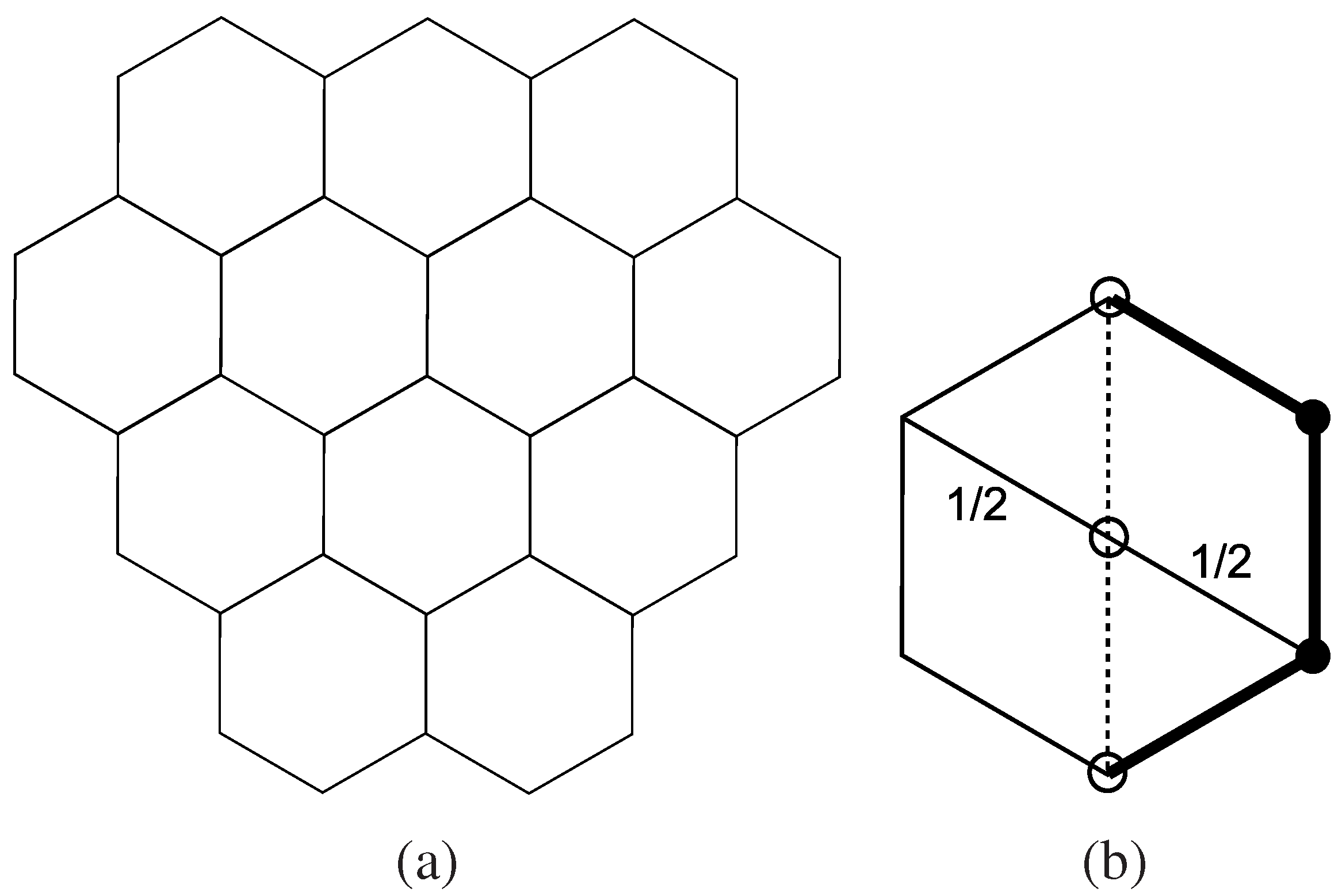
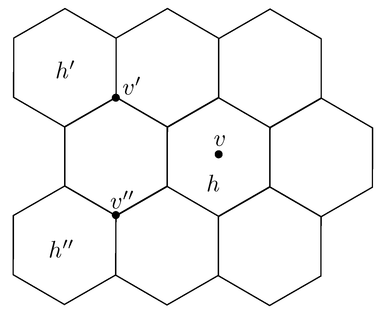
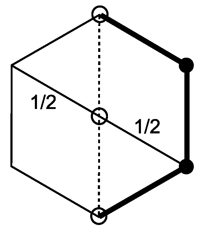
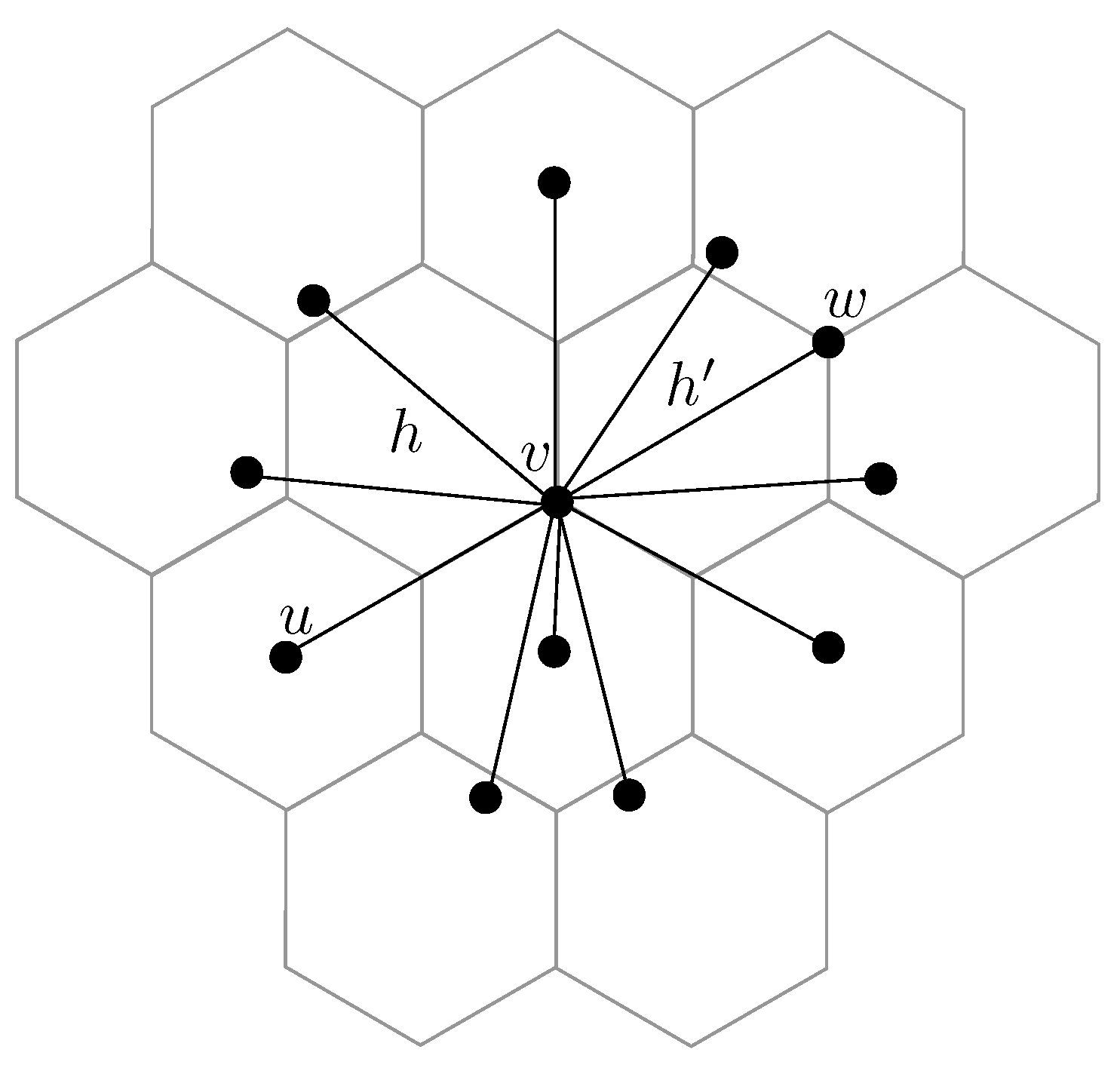
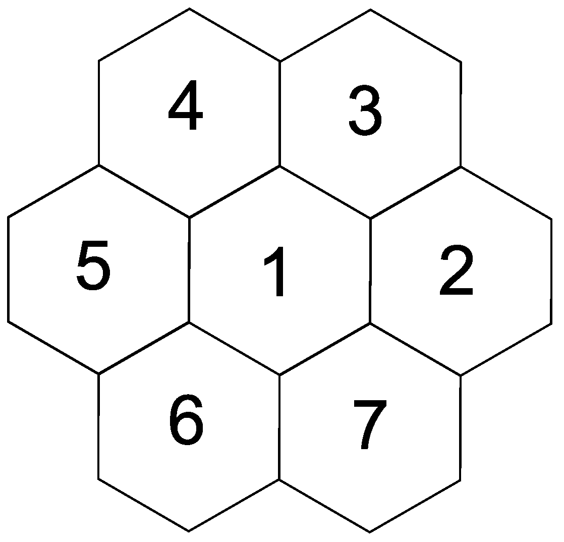
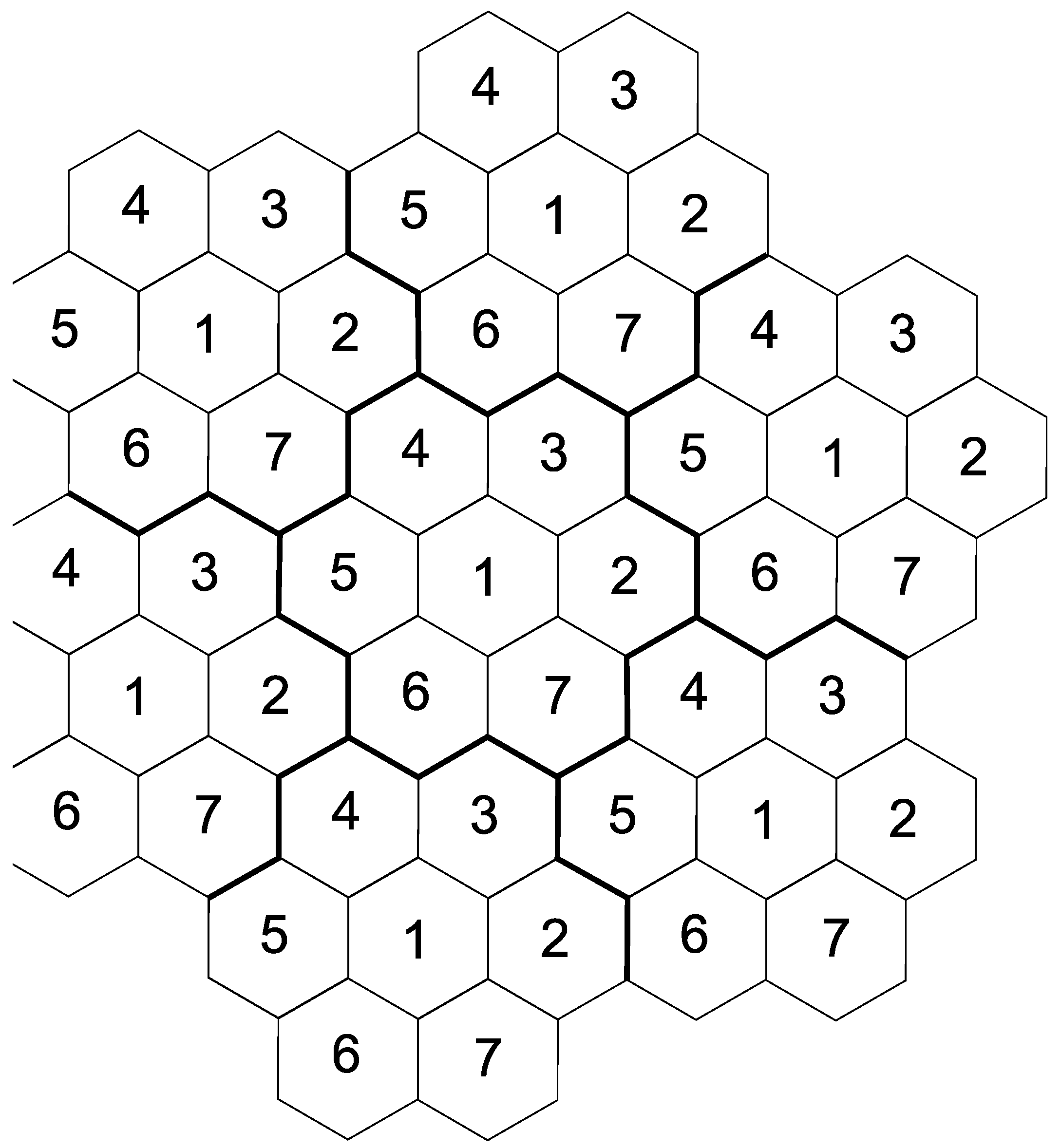
2.1. Tiling of the Plane

We tile the plane in hexagons in a way that achieves the following properties:
  • Each vertex is contained in exactly one hexagon.
  • All vertices in a hexagon are connected by an edge.
We attain the above properties by tiling the plane in hexagons with a diameter of one. Ambiguities caused by vertices at the border of hexagons are resolved as shown in Figure 1 (b): The right borders excluding the upper and lower apexes belong to a hexagon, the rest of the border does not. We assume that the tiling starts with the coordinates (0,0) being in the center of a tile of class 1.
This is similar to the tiling used in [17] but in contrast to their tiling our hexagons do not have any information that distinguishes them from one another (class numbers, etc.).

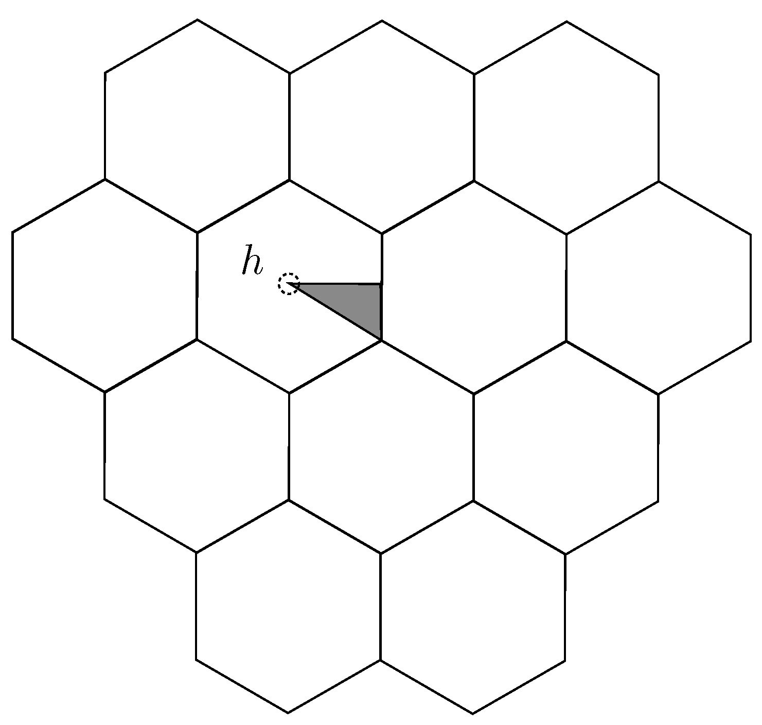
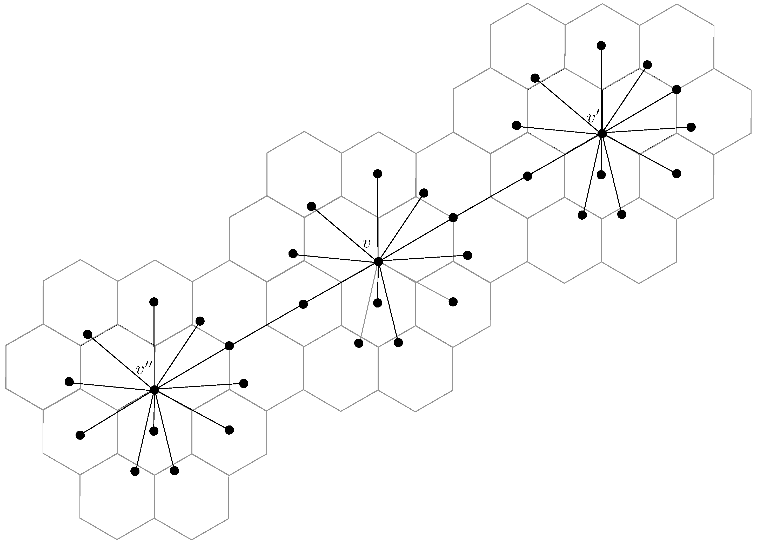
2.2. Algorithm for Unit Disk Graphs

Now we present a local algorithm for dominating set on unit disk graphs (UDGs) with locality one. Let G = (V, E) be a unit disk graph. The algorithm works as follows: In each hexagon h the vertex v which is closest to the center of h is assigned to the dominating set D. Ambiguities are resolved by e.g., choosing the vertex with the smallest x-coordinate. We refer to this as Algorithm 1.
We prove the correctness of Algorithm 1 in Theorem 1.
Theorem 1. 
Let G be a unit disk graph. Algorithm 1 has the following properties:
1.
The computed set D is a dominating set for G.
2.
Let DOPT be an optimal dominating set. It holds that |D| ≤ 12 · |DOPT|.
3.
Whether or not a vertex v is in D depends only on the vertices at most one hop away from v, i.e. Algorithm 1 is local.
4.
The processing time for a vertex v is linear in the number of vertices adjacent to v.
Algorithm 1: Local algorithm for finding a dominating set in a unit disk graph
1 // Algorithm is executed independently by each node v;
2 // Denote by Vh all vertices in h;
3 Find all vertices in N(v) and compute Vh;
4 if v is the vertex closest to the center of h among all v′Vh then become part of D else Do not become part of D
Proof. 
We first prove that D is indeed a dominating set for G. Let h be a non-empty hexagon and denote by Vh all vertices in h. As Vh ≠ ∅ it holds that one vertex vVh is the vertex which is closest to the center of h. So vD and v dominates all vertices in h.
Now we prove that for an optimal dominating set DOPT it holds that |D| ≤ 12 · |DOPT|. In the following we prove that for any vertex in DOPT there can exist at most 12 hexagons that have a vertex at (Euclidean) distance at most one from it. (In fact this holds for all vertices but we need the claim only for vertices in DOPT.) Consider a vertex vDOPT in a hexagon h. Without loss of generality we assume that v is in the gray area of h as shown in Figure 3 or in the center of h as shown in Figure 2. In both cases for a vertex v′D that is adjacent to v it holds that v′ must be in one of the 9 or 12 hexagon in the respective figure (for the case of v being in the center of h check the resolving method for ambiguities at the border of hexagons, Figure 1b). Since at most one vertex per hexagon was assigned to D there are at most 12 vertices in D that are adjacent to v. (Note that in the case where v is in the gray area the resolving method for ambiguities does not come into play.)
So for each vertex vDOPT it holds that it is adjacent to at most 12 vertices in D. Since DOPT is a dominating set all vertices in D must be adjacent to at least one vertex in DOPT. This leads to |D| ≤ 12 · |DOPT|.
Next we determine the locality of Algorithm 1. In the algorithm, a vertex v in a hexagon h only needs to explore all vertices which are at most one hop away from v in order to determine whether v is the vertex closest to the center of h. So whether or not vD depends only on the vertices which are at most one hop away from v.
Now we prove the processing time of Algorithm 1. Let v be a vertex and define n1(v) := |N1(v)|. In the algorithm v needs to determine for each vertex v′N1(v) whether v′h and whether v′ is closer to the center of h than v. This can be done in O (n1(v)) time. ☐

2.3. Tightness of Approximation Factor

We give an example which shows that our analysis of Algorithm 1 is tight. Consider the graph shown in Figure 4 and denote it by G (we omitted the edges which are not adjacent to v in order to make the figure clearer). Note that the vertex v is on the crossing of three hexagons but is assigned to the hexagon h. The vertex w is on a crossing of three hexagons as well but by our resolving method it is assigned to the hexagon h′. Also note that the vertex u is directly in the center of its hexagon. We observe that the vertex v alone is sufficient to dominate all other vertices in G. Since each hexagon contains only one vertex, Algorithm 1 assigns every vertices in the graph to D. So Algorithm 1 achieves a competitive ratio of 12 in G.
We can enlarge this construction to an arbitrary size by putting several copies of G together. This is shown in Figure 5. The copies of G are indeed connected since the length of an edge of a hexagon is 1/2 and the diameter of a hexagon is 1.

2.4. Lower Bound

Here we present a construction which enables us to give a lower bound for the approximation factor of a local algorithm for dominating set with a locality distance of k.
Theorem 2. 
Let 𝒜 be a local algorithm for dominating set in unit line graphs with locality distance k in the setting of location aware nodes. The best performance ratio which can be achieved by 𝒜 is
Algorithms 01 00002 i001
i.e., for arbitrary k the best performance ratio is 1 + 3 2 k + ( ( k 1 ) mod 3 ) + 1 .
Proof. 
Consider the unit line graph G = (V, E) consisting of 4 + 2k vertices (see Figure 6). Denote by VM the four vertices in the middle. Let D be the dominating set which is computed by 𝒜 for G. We distinguish three cases:
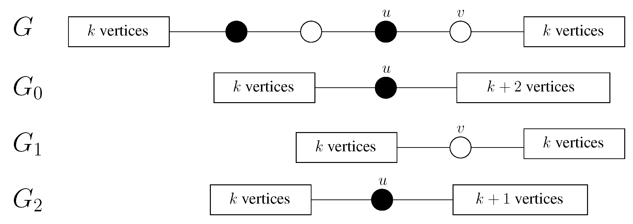
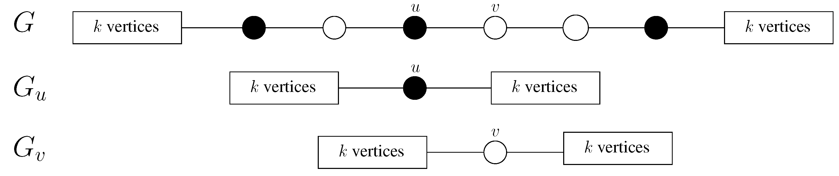
  • k ≡ 0 mod 3. Then there must be at least one vertex uVM such that uD (otherwise D would not be a dominating set). Consider the graph G0 consisting of u and k vertices on the left and k + 2 vertices on the right of u (see Figure 6). Let D0 be the dominating set which is computed by 𝒜 for G0. An optimal dominating set for G0 has 2 k + 3 3 vertices. However, as uD and the locality of 𝒜 is k it follows that uD0. Therefore it follows that |D0| ≥ k 1 3 + 1 + k + 1 3 = 2 k + 6 3 . So the approximation ratio of 𝒜 is a least 2 k + 6 3 / 2 k + 3 3 = 2 k + 6 2 k + 3 = 1 + 3 2 k + 3 .
  • k ≡ 1 mod 3. We distinguish whether or not there are vertices in VM which are not in D. If all vertices in VM are in D then it holds that |D| ≥ k 1 3 + 4 + k + 1 3 = 2 k + 10 3 . However, an optimal dominating set for G has at most 2 k + 4 3 vertices. So then the approximation ratio of 𝒜 is at least 2 k + 10 3 / 2 k + 4 3 = 2 k + 10 2 k + 4 = 1 + 6 2 k + 3 .
    If there is a vertex vVM with vD then we consider the graph G1 which consists of v and k vertices on the left and on the right of v (see Figure 6). Let D1 be the dominating set which is computed by 𝒜 for G1. An optimal dominating set for G1 has 2 k + 1 3 vertices. However, as vD and the locality of 𝒜 is k it follows that vD1. This implies that |D1| ≥ k 1 3 + 2 + k + 1 3 = 2 k + 4 3 . So the approximation ratio of 𝒜 is a least 2 k + 4 3 / 2 k + 1 3 = 2 k + 4 2 k + 1 = 1 + 3 2 k + 1 . As 1 + 3 2 k + 1 ≤ 1 + 6 2 k + 3 it follows that if k ≡ 1 mod 3 then the approximation ratio of 𝒜 is a least 1 + 3 2 k + 1 .
  • k ≡ 2 mod 3. Then there must be at least one vertex uVM such that uD (otherwise D would not be a dominating set). Consider the graph G2 consisting of u and k vertices on the left and k + 1 vertices on the right of u (see Figure 6). Let D2 be the dominating set which is computed by 𝒜 for G2. An optimal dominating set for G2 has 2 k + 2 3 vertices. However, as uD and the locality of 𝒜 is k it follows that uD0. Therefore it follows that |D0| ≥ k 1 3 + 1 + k 3 = 2 k + 5 3 . So the approximation ratio of 𝒜 is a least 2 k + 5 3 / 2 k + 2 3 = 2 k + 5 2 k + 2 = 1 + 3 2 k + 2 .
Corollary 1. 
Let 𝒜 be a local algorithm for dominating set in unit disk graphs (UDGs) with a locality distance of k hops in the setting of location aware nodes. The best performance ratio which can be achieved by 𝒜 is
Algorithms 01 00002 i001

2.5. Algorithm for Unit Line Graphs

We present a local algorithm for dominating set on unit line graphs (ULGs) with locality one. It achieves an approximation ratio of 3. The idea is to divide the line into units of width one. Then we assign one vertex from each unit to the dominating set.
Now we present the algorithm in detail. Let G = (V, E) be a unit line graph. For a vertex v we denote by vx its x-coordinate. For all integers i we define Vi := {vV|ivx < i + 1}. We define H := {i|Vi ≠ ∅}. For all iH we define v[i] to be the vertex with the smallest x-coordinate in Vi. We define D := {v[i]|iH}. We output D. We refer to this as Algorithm 2.
Algorithm 2: Local algorithm for finding a dominating set in a unit line graph
1 // Algorithm is executed independently by each node v;
2 // let i be the integer such that vVi;
3 // let v[i] be vertex with the smallest x-coordinate in Vi;
4 Find all vertices in N(v) and determine Vi;
5 if v = v[i] then become part of the dominating set D else Do not become part of D
We prove the correctness of Algorithm 2 in Theorem 3.
Theorem 3. 
Let G be a unit line graph. Algorithm 2 has the following properties:
1.
The computed set D is a dominating set for G.
2.
Let DOPT be an optimal dominating set. It holds that |D| ≤ 3 · |DOPT|.
3.
Whether or not a vertex v is in D depends only on the vertices at most one hop away from v, i.e. Algorithm 2 is local.
4.
The processing time for a vertex v is linear in the number of vertices adjacent to v.
Proof. 
We first prove that D is indeed a dominating set for G. Let iH. As Vi ≠ ∅ it holds that v[i] ∈ ViD. So v[i] dominates all vertices in Vi.
Now we prove that for an optimal dominating set DOPT it holds that |D| ≤ 3 · |DOPT|. Consider a vertex vDOPT in a set Vi. Since all sets Vj have width one it holds that v is adjacent to at most 3 vertices in D (at most one each in Vi − 1, Vi, and Vi + 1). Since DOPT is a dominating set all vertices in D must be adjacent to at least one vertex in DOPT. This leads to |D| ≤ 3 · |DOPT|.
Next we determine the locality of Algorithm 2. In the algorithm, a vertex v in a set Vi only needs to explore all other vertices in Vi. (This is sufficient to determine whether v is the vertex with the smallest x-coordinate among the vertices in Vi.) So whether or not vD depends only on the vertices which are at most one hop away from v.
Now we prove the processing time of Algorithm 2. Let v be a vertex and define n1(v) := |N1(v)|. In the algorithm v needs to determine for each vertex v′N1(v) whether v′Vi and whether v′ has a smaller x-coordinate than v. This can be done in O (n1(v)) time.  ☐

3. Connected Dominating Set

In this section we present a local approximation algorithm that computes a factor 216 approximation for connected dominating set. We prove its correctness, its approximation ratio and its locality distance of two hops. We prove that in contrast to the other problems discussed in this paper there is no constant ratio approximation algorithm with locality distance one. We give lower bounds for the approximation ratio of local algorithms with arbitrary locality distance k. Finally we give an approximation algorithm for connected dominating set for unit line graphs which achieves an approximation factor of 6.

3.1. Algorithm for Unit Disk Graphs

We present our approximation algorithm for connected dominating set in unit disk graphs with locality two. Let G = (V, E) be a connected unit disk graph. We use the same tiling of the plane as introduced in Section 2. The algorithm works as follows: Consider one hexagon h. We consider each hexagon h′ such that there are pairs of adjacent vertices v and v′ with vh, v′h′. We compute the two adjacent vertices vh, v′h′ which are closest to each other (ties are resolved by some resolving method, e.g., by choosing the pair where the vertex in h has the smallest x-coordinate etc.). We assign v and v′ to the connected dominating set CD. Do this for all hexagons h′ with the above property.
If there are no such hexagons h′ we assign the vertex vh to CD which is closest to the center of h (ties are broken like in Algorithm 1). The above description is presented in Algorithm 3.
We prove the correctness and the other properties of Algorithm 3 in Theorem 4.
Theorem 4. 
Let G be a unit disk graph. Algorithm 3 has the following properties:
1.
The computed set CD is a connected dominating set for G.
2.
Let CDOPT be an optimal connected dominating set. It holds that |CD| ≤ 216 · |CDOPT|.
3.
Whether or not a vertex v is in CD depends only on the vertices, i.e. Algorithm 3 is local.
4.
The processing time for a vertex v is quadratic in the number of vertices adjacent to v.
Proof. 
First we prove that the set CD is indeed a connected dominating set for G. From the construction it follows that in each hexagon which contains vertices of G at least one vertex is assigned to CD. So CD is a dominating set for G. If in G a vertex v ¯ in a hexagon h is adjacent to a vertex v ¯ in a hexagon h′, then the algorithm ensures that for two adjacent vertices v and v′ with vh and v′h′ it holds that vCD and v′CD. So in G there is an edge between two vertices in two different hexagons if and only if in G restricted to CD there is an edge between these hexagons. It follows that CD is connected since G is connected.
Algorithm 3: Local algorithm for finding a connected dominating set in a unit disk graph
Algorithms 01 00002 i002
Now we want to prove the approximation ratio of Algorithm 3. In Algorithm 1 at most one vertex per hexagon is assigned to the connected dominating set. We showed in Theorem 1 that this ensures an approximation ratio of 12 in comparison with an optimal dominating set. Now for one hexagon h there are at most 18 hexagons h′ such that there are edges between vertices in h and h′. So at most 18 vertices from h are assigned to CD. Let DOPT be an optimal dominating set, let CDOPT be an optimal connected dominating set and let D be the dominating set computed by Algorithm 1. It follows that
Algorithms 01 00002 i003
Now we prove the locality of Algorithm 3. Consider a vertex v in a hexagon h. In order to find out whether or not v is assigned to CD we need to find out whether v is adjacent to a vertex v′ in a hexagon h′ with hh′ and what other vertices v ¯ h are adjacent to vertices v ¯ h′. In order to do this, we need to explore all vertices which are at most two hops away from v. To check whether there are generally vertices in h which are adjacent to vertices in other hexagons (if not, the vertex closest to the center of h is assigned to CD), we need to explore the vertices which are at most two hops away from v.
Finally we prove the processing time of Algorithm 3. Let again v be a vertex in a hexagon h. We define n2(v) := |N2(v)|. For each vertex v′N1(v) the vertex v needs to determine whether v′h and to what vertices v ¯ in other hexagons h′ the vertex v′ is adjacent to. For each hexagon h′ such that there are adjacent vertices in h and h′ we need to compute the pair of vertices vh and v′h′ which are closest to each other and need to compute the resolving of the ties. This can be done in O (n2(v)2) time. ☐

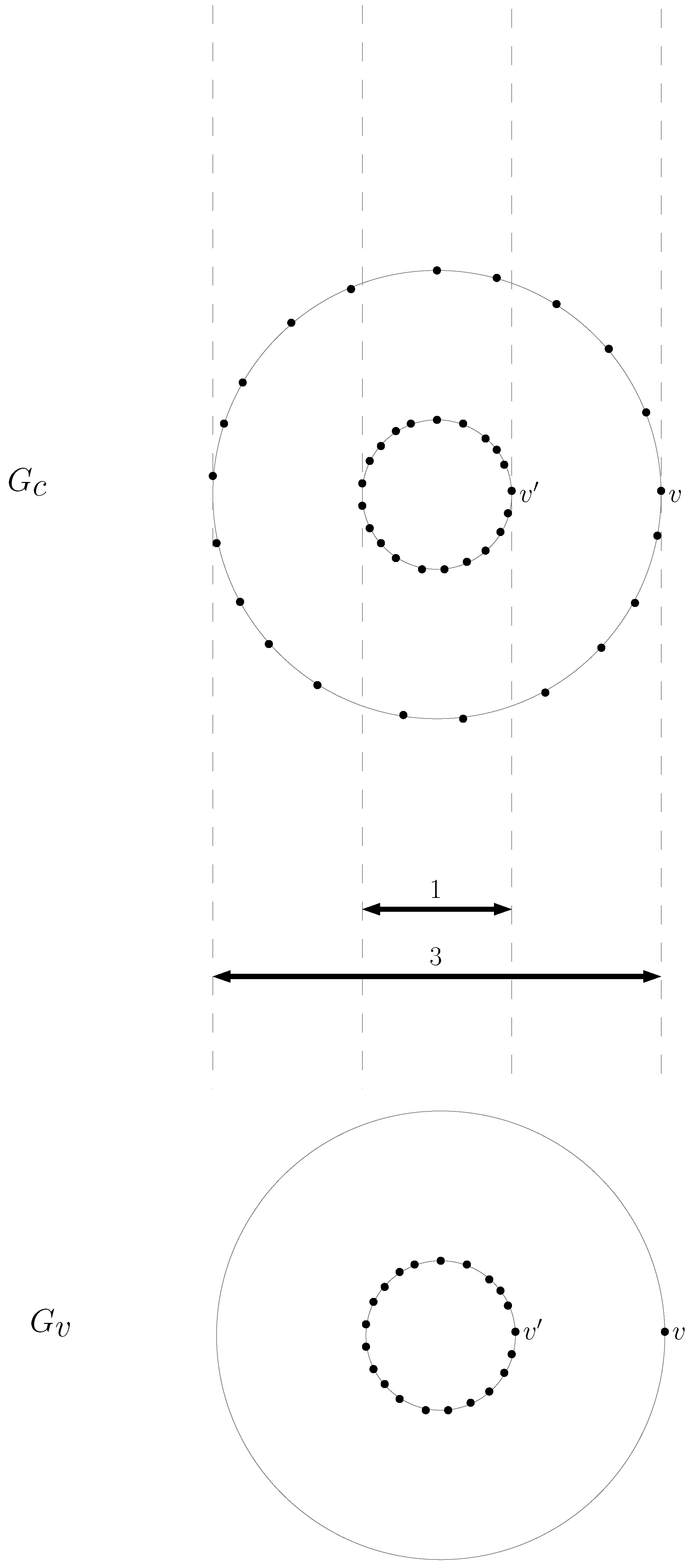
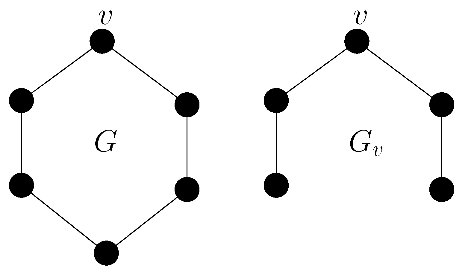
3.2. No Constant Ratio Approximation Algorithm with Locality One

We prove that there is no local algorithm for connected dominating set with locality one which achieves a constant approximation ratio.
Theorem 5. 
Let 𝒜 be a local algorithm with locality one for connected dominating set in the setting of location aware nodes. For every constant c there is a graph Gc such that 𝒜 achieves an approximation ratio worse than c when computing a connected dominating set for Gc.
Proof. 
Without loss of generality we assume that c is an integer. Consider two circles of diameters one and three which are placed inside of each other (see Figure 7). Consider the unit disk graph Gc defined as follows: There are 21 · c vertices distributed on the inner ring. Denote these vertices by VI. On the outer ring there are another 21 · c vertices such that each of them is opposite to one vertex in VI. We denote by VO the vertices on the outer ring. Since Gc is a unit disk graph an edge between two vertices exists if and only if the Euclidean distance between the vertices is at most one. For each vertex vVO we define the unit disk graph Gv as follows: it consists of the vertices VI and the vertex v. Denote by v′ the vertex opposite of v on the inner ring. Again, an edge between two vertices exists if and only if the Euclidean distance between two vertices is at most one. Figure 7 shows this construction for c = 1. When 𝒜 computes a connected dominating set CDv for Gv it holds that v′CDv (since v must be dominated either by v′ or by v itself which implies for CDv to be connected that v′ must be in CDv as well). When 𝒜 computes a connected dominating set CD for Gc it must take the same decision about assigning v′ to CD as in Gv (since the locality of 𝒜 is one). So v′CD. With the same argument we can show that for every vertex uVI it holds that uCD. So VICD and therefore |CD| ≥ 21 · c. But since the length of the outer ring is 3π it holds that the size of a maximal independent set is at most ⌊3π⌋ = 10 and therefore the size of a connected dominating set for Gc is at most 20 (we can construct this by taking a maximal independent subset IO of VO and add all vertices in VI which are opposite of vertices in IO). Denote by CDOPT an optimal dominating set for Gc. So for the approximation ratio |CD|/|CDOPT| it holds that
Algorithms 01 00002 i004
Corollary 2. 
Let 𝒜 be a local algorithm with locality one for connected dominating set in the setting of location aware nodes. The approximation ratio of 𝒜 is bounded from below by n/40, i.e., it is in Θ(n).
Proof. 
We apply the construction in the proof of Theorem 5 to obtain the family of graphs Gc. For each graph Gc the following holds: Let CD be the connected dominating set for Gc which is computed by 𝒜. All vertices in the inner ring are assigned to CD by 𝒜 (see the proof of Theorem 5). As half of the vertices of Gc are on the inner ring, it holds that |CD| ≥ n/2. However, an optimal connected dominating set CDOPT for Gc has at most 20 vertices, so |CDOPT| ≤ 20. So for the approximation ratio |CD|/|CDOPT| it holds
Algorithms 01 00002 i005

3.3. Lower Bound

We prove a lower bound for the approximation factor of local algorithms for connected dominating set in the setting of location aware nodes depending on the locality distance of the algorithm.
Theorem 6. 
Let 𝒜 be a local algorithm for connected dominating set in the setting of location aware nodes. Let k be the locality distance of 𝒜. Then the approximation ratio which 𝒜 achieves is bounded from below by 1 + 1/k.
Proof. 
Similar to the proof of Theorem 2 we construct graphs in which 𝒜 has to take the same decisions in a certain vertex v. Our construction consists of a cycle of vertices with 2k + 2 vertices as shown in Figure 8. Denote this cycle by G. Note that G is indeed a unit disk graph. Denote by CD the connected dominating set which 𝒜 computes for G. Now let v be a vertex. Denote by Gv the graph which we obtain by removing the opposite vertex of v from G (see Figure 8). As 𝒜 is a local algorithm with locality distance k it must take the same decision about assigning v to the connected dominating set in G and Gv. Denote by CDv the connected dominating set which is computed for Gv by 𝒜. As not assigning v to CDv would result in CDv being disconnected, we conclude that vCDv and vCD. With the same reasoning we can show that all vertices in G must be in CD. So |CD| = 2k + 2. But an optimal connected dominating set for G has only 2k vertices. So the performance ratio of 𝒜 is bounded from below by 2 k + 2 2 k = 1 + 1 k .
Corollary 3. 
Let 𝒜 be a local algorithm for connected dominating set in the setting of location aware nodes with locality distance 2. Then the approximation ratio which 𝒜 achieves is bounded from below by 1.5.

3.4. Algorithm for Unit Line Graphs

We present a local algorithm for connected dominating set on unit line graphs with locality distance one. It is an extension of the algorithm for dominating set presented in this paper. The approximation ratio of this algorithm is 6.
Now we present the algorithm in detail. Let G = (V, E) be a unit line graph. For a vertex v we denote by vx its x-coordinate. As in Algorithm 2 for all integers i we define Vi := {vV|ivx < i + 1} and H := {i|Vi ≠ ∅}. For all iH we define v[i] and v′[i] to be the vertices with the smallest and largest x-coordinates in Vi. We define CD:= {v[i], v′[i]|iH}. We output CD. We refer to this as Algorithm 4.
Algorithm 4: Local algorithm for finding a connected dominating set in a unit line graph
1 // Algorithm is executed independently by each node v;
2 // let i be the integer such that vVi;
3 Find all vertices in N (v) and determine Vi;
4 if v = v[i] or v = v′[i] then become part of the dominating set CD else Do not become part of CD
We prove the correctness of Algorithm 4 in Theorem 7.
Theorem 7. 
Let G be a unit line graph. Algorithm 4 has the following properties:
1.
The computed set CD is a connected dominating set for G.
2.
Let CDOPT be an optimal connected dominating set. It holds that |D| ≤ 6 · |DOPT|.
3.
Whether or not a vertex v is in CD depends only on the vertices at most one hop away from v, i.e. Algorithm 4 is local.
4.
The processing time for a vertex v is linear in the number of vertices adjacent to v.
Proof. 
We first prove that CD is indeed a connected dominating set for G. Let iH. Let D be the dominating set which Algorithm 2 would have computed for G. As DCD it remains to prove that CD is connected. For all i it holds that v[i] and v′[i] are connected by an edge (assuming v[i] ≠ v′[i]). Let i be an integer such that iH and i + 1 ∈ H. Then there are edges connecting v′[i] and v[i+ 1] since v′[i] is the vertex on the very right of Vi and v[i + 1] is the vertex on the very left of Vi + 1 and G is a connected unit line graph. This proves that CD is connected.
Now we prove that for an optimal connecting dominating set CDOPT it holds that |CD| ≤ 6 · |CDOPT|. Let D again be the dominating set which Algorithm 2 would have computed for G. From our construction it follows that |CD| ≤ 2 · |D|. As |DOPT| ≤ |CDOPT| it follows that
Algorithms 01 00002 i006
Next we determine the locality of Algorithm 4. In the algorithm, a vertex v in a set Vi only needs to explore all other vertices in Vi. (This is sufficient to determine whether v is the vertex with the smallest x-coordinate or with the largest x-coordinate among the vertices in Vi.) So whether or not vCD depends only on the vertices which are at most one hop away from v.
Now we prove the processing time of Algorithm 4. Let v be a vertex and define n1(v) := |N1(v)|. In the algorithm v needs to determine for each vertex v′N1(v) whether v′Vi and whether v′ has a smaller or a larger x-coordinate than v. This can be done in O (n1(v)) time. ☐

4. Independent Set

In this section we present our local approximation algorithm for independent set in unit disk graphs with locality one. This algorithm achieves an approximation ratio of 1/1801. Then we give a lower bound for the approximation ratio of local algorithms with arbitrary locality distance k. For this proof we employ a construction consisting of unit line graphs. Finally we give a local algorithm for unit line graphs with locality one. Its approximation ratio is almost 1/2.
First we introduce another tiling of the plane which is a bit more complex than the tiling presented in Section 2.

4.1. Tiling of the Plane

We present the tiling of the plane which our local algorithm for independent set in UDGs will use. Let G = (V, E) be a connected unit disk graph. We tile the plane with tiles where each tile consists of seven hexagons arranged as in Figure 9. The diameter of each hexagon is 1. Each hexagon is assigned a class number between 1 and 7. This assignment is done identically in each tile. For a hexagon h we denote by class(h) its class number. Each vertex is assigned to a hexagon, ambiguities caused by vertices at the border of hexagons are resolved as shown in Figure 10 (this is the same resolving method which was used in Section 2.1.). The plane is tiled with the tiles mentioned above as shown in Figure 11. We conclude with the following proposition.
Proposition 1. 
Two different hexagons with the same class number have an Euclidean distance of strictly more than 1.

4.2. lgorithm for Unit Disk Graphs

We present our local approximation algorithm for independent set in unit disk graphs. Let G = (V, E) be a unit disk graph. The main idea of the algorithm is that since the vertices in one hexagon form a clique at most one vertex per hexagon can be in an independent set. The algorithm works as follows: In each hexagon h we define the vertex which is closest to the center to be the head vertex vh (ambiguities are resolved by choosing the vertex with the smallest x-coordinate among the vertices with the same distance to the center and if this is ambiguous we choose the vertex with the smallest y-coordinate). If vh is not adjacent to a vertex in a hexagon with a lower class number we assign vh to the independent set I.
Algorithm 5: Local algorithm for finding an independent set in a unit disk graph
Algorithms 01 00002 i007
We prove the correctness of Algorithm 5, its approximation factor, its locality and its processing time in Theorem 8.
Theorem 8. 
Let G be a unit disk graph. Algorithm 5 has the following properties:
1.
The computed set I is an independent set for G.
2.
Let IOPT be an optimal independent set. It holds that|I| ≥ 1 1801 |IOPT|.
3.
Whether or not a vertex v is in I depends only on the vertices at most one hop away from v, i.e. Algorithm 5 is local.
4.
The processing time for a vertex v is linear in the number of vertices adjacent to v.
Proof. 
First we want to show that I is indeed an independent set for G. Assume on the contrary that there are two adjacent vertices vI and v′I. Since at most one vertex per hexagon is assigned to I it follows that v and v′ are in different hexagons h and h′ respectively. From Proposition 1 it follows that class(h) ≠ class(h′), so without loss of generality we can assume that class(h) > class(h′). But from the construction it follows that a vertex v in a hexagon h is not assigned to I if it is adjacent to a vertex v′ in a hexagon h′ with class(h) > class(h′). This is a contradiction. So the set I is an independent set for G.
Now we want to prove the approximation ratio of Algorithm 5. Let IOPT be an optimal independent set for G. Denote by H the set of hexagons which contain vertices from G. Since the vertices in a hexagon form a clique, at most one vertex per hexagon can be part of an independent set. So |H| is an upper bound for |IOPT|. For a hexagon h we denote by B(h) the union of h and all hexagons h′ such that class(h) < class(h′) and h′ contains a vertex which is adjacent to a vertex in h. For a set of hexagons H′ we define B(H′) := ∪h′H′ B(h′). We define recursively B0(h) := {h} and Bi(h) := B(Bi − 1(h)). As there are only seven different classes of hexagons, it follows that B7 − i(h) = B7 − i+k(h) for hexagons of class i and for all k ≥ 0. We define B ˜ (h) := B7 − class(h)(h). Intuitively we can say that the hexagon h blocks all hexagons in B ˜ (h).
Consider a graph G′ = (V′, E′) with one vertex per hexagon in H and with an edge between two vertices if and only if their respective hexagons are adjacent. For two hexagons h,h′ we denote by d(h, h′) the distance between their respective vertices in G′. For a hexagon h we get that for all hexagons h′ B ˜ (h) it holds that d(h, h′) ≤ 2. So for all hexagons h′ B ˜ (h) it holds that d(h, h′) ≤ 2 (7 − class(h)) ≤ 12. As for a hexagon h there are at most 3(2k)2 + 3(2k) + 1 hexagons h′ such that d(h, h′) ≤ k (see the proof of Lemma 6 in [18]) we conclude that | B ˜ (h)| ≤ 3 · 242 + 3 · 24 + 1 = 1801. It follows that 1801|I| ≥ ∪v′I | B ˜ (h(v′))|.
For a vertex v let h(v) be the hexagon which contains v. From the definition of the algorithm we get the following: Let v be a head vertex. If for all vertices v′I it holds that h(v) ∉ B ˜ (h(v′)) then it holds that vI. So ∪v′I B ˜ (h(v′)) = H. We conclude that
Algorithms 01 00002 i008
Now we want to prove the locality of Algorithm 5. Since a vertex only needs to determine whether it is the head vertex of its hexagon and whether it is adjacent to a vertex in a hexagon with lower class number, the locality distance of the algorithm is one hop.
For the proof of the processing time let v be a vertex in a hexagon h. For each vertex v′N (v) the algorithm needs to compute the class number of the hexagon containing v′ and its distance to the center of h. This can be done in O (|N (v)|) time. ☐

4.3. Lower Bound

Similarly to the lower bound presented in Section 2.4. we present a construction which enables us to give a lower bound for the approximation factor of local algorithms for independent set with a locality distance of k hops.
Theorem 9. 
Let 𝒜 be a local algorithm for independent set in unit line graphs with a locality distance of k hops in the setting of location aware nodes. The best performance ratio which can be achieved by 𝒜 is k k + 1 .
Proof. 
Consider the unit line graph G1 = (V, E) consisting of 6 + 2k vertices (see Figure 12). Let I1 be the independent set which is computed for G1 by 𝒜. Note that an optimal independent set for G1 has k + 3 vertices. Let V1 be the set of vertices in G1 which are at most k − 1 hops away from the very right or the very left vertex (in Figure 12 these are the vertices in the box with the label “k vertices”). If k = 0 we define V1 := ∅. Let V2 := V\V1 (thus |V2| = 6). We distinguish three cases:
Case 1: There is no vertex uV2 such that uI1. If k = 0 then |I1| = 0 and thus the performance ratio of 𝒜 is 0. If k ≥ 1 then |I1| ≤ k + 1 and so the performance ratio of 𝒜 is at most k + 1 k + 3 k k + 1 .
Case 2: There is no vertex vV2 such that vI1. Then I1 is not an independent set which is a contradiction.
Case 3: There is a vertex uV2 with uI1 and a vertex vV2 with vI1. Now consider the graphs Gu consisting of u and v respectively and k nodes each to their left and their right (see Figure 12). Let Iu and Iv be the independent sets computed for Gu and Gv by 𝒜. As the locality distance of 𝒜 is k and uI1 and vI1, it holds that uIu and vIv. If k is even then |Iv| ≤ k whereas the optimal independent set for Iv has k + 1 vertices. So the performance ratio of 𝒜 is at most k k + 1 . If k is odd then |Iu| ≤ k whereas the optimal independent set for Iu has k + 1 vertices. So the performance ratio of 𝒜 is k k + 1 . ☐
Corollary 4. 
Let 𝒜 be a local algorithm for independent set in unit disk graphs (UDGs) with a locality distance of k hops in the setting of location aware nodes. The best performance ratio which 𝒜 can achieve is k k + 1 .

4.4. Algorithm for Unit Line Graphs

We present a local algorithm for independent set with locality one on unit line graphs (ULGs). For the set I computed by this algorithm it holds that |I| ≥ ⌊ 1 2 · |IOPT|⌋ and |I| ≥ 1 (with IOPT being an optimal independent set). Like in Algorithm 2 we divide the line into units of width one.
Now we present the algorithm in detail. Let G = (V, E) be a unit line graph. For a vertex v we denote by vx its x-coordinate. For all integers i we define Vi := {vV|ivx < i + 1}. We define H := {i|Vi ≠ ∅}. For all iH we define v[i] to be the vertex with the smallest x-coordinate in Vi. Now we partition the vertices v[i] into two sets V1 and V2. Let V1 := {v[i]|iHi is odd} and V2 := {v[i]|iHi is even}. Denote by V′V2 the subset of V2 consisting of the vertices v[i] which are not adjacent to vertices v′ with v′Vi − 1 or v′Vi + 1 (so for such a vertex v′ it would hold that v x < i or v x ≥ 1). We define the independent set I as I := V1 V 2 . The output is the set I. We refer to this as Algorithm 6.
We prove the correctness of Algorithm 6, its approximation factor, its locality and its processing time in Theorem 10.
Algorithm 6: Local algorithm for finding an independent set in a unit line graph
Algorithms 01 00002 i009
Theorem 10. 
Let G be a unit line graph. Algorithm 6 has the following properties:
1.
The computed set I is an independent set for G.
2.
Let IOPT be an optimal independent set. It holds that|I| ≥ ⌊ 1 2 · |IOPT|⌋ and|I| ≥ 1.
3.
Whether or not a vertex v is in I depends only on the vertices which are at most k hops away from v, i.e. Algorithm 6 is local.
4.
The processing time for a vertex v is linear in the number of vertices adjacent to v.
Proof. 
It holds that the Euclidean distance between two vertices in V1 is strictly greater than one. So V1 is an independent set. Since all vertices in V 2 are not adjacent to vertices v′ with v′ < i or v x i + 1 it holds that a vertex in V 2 cannot be adjacent to a vertex in V1. Like for V1 it holds that the Euclidean distance between two vertices in V2 is strictly greater than one. So no two vertices in V 2 are adjacent. All this implies that I = V1 V 2 is in independent set.
Now we want to prove the approximation ratio of Algorithm 6. Let i be an integer. The vertices in Vi form a clique. Therefore at most one vertex in Vi can be in I. So |H| is an upper bound for |IOPT|. If |H| is even then |V1| = | H | 2 . If |H| is odd then either |V1| = | H | + 1 2 or |V1| = | | H | 1 2 . So in either case it holds that |I| ≥ |V1| ≥ ⌊ 1 2 · |IOPT|⌋. If |V1| ≥ 1 it clearly holds that |I| ≥ 1. If |V1| = 0 there must be one set Vi with Vi ≠ ∅ and i being even (since otherwise the graph would be empty and for the empty graph the theorem is trivially true). It also holds that Vi − 1 = ∅ and Vi + 1 = ∅. So v[i] is not adjacent to any vertices in Vi − 1 or Vi + 1 and therefore v[i] ∈ I. This implies that |I| ≥ 1.
Let vVi be a vertex. In order to determine whether vI we need to explore the vertices in Vi and we need to determine whether v is adjacent to a vertex v′ with v′Vi − 1 or v′Vi + 1. All this requires only the knowledge of the vertices in N(v). So the locality distance of Algorithm 6 is one. Computing whether v = v[i] and whether v is adjacent to a vertex v′ with v′Vi − 1 or v′Vi + 1 can be done in processing time linear in |N(v)|. ☐

5. Vertex Cover

In this section we prove that if we take all vertices in a unit disk graph this forms a factor 6 approx-imation for the minimum vertex cover problem. This leads to a local approximation algorithm with a locality of one hop. Then we present lower bounds for the approximation ratio of local algorithms for vertex cover with arbitrary locality distance k. Finally we give a factor 2 approximation algorithm for vertex cover on unit line graphs.

5.1. Factor 6 Upper Bound

We consider a connected unit disk graph with at least two vertices. An upper bound of 6 for the number of all vertices in comparison with the number of vertices in a minimum vertex cover follows from Theorem 11 for m = 6 (recall that a unit disk graph does not contain a K1,6 minor).
Theorem 11. 
Let G = (V, E) be a graph such that there is no set of vertices V′ ⊆ V such that the subgraph induced by V′ is a K1,m. Then it holds that
|V| ≤ m · |V COPT|
Proof. 
We partition the vertices V into two sets V1 := V COPT and V2 := V\V1. We prove that |V2| ≤ (m − 1) · |V COPT|. Since |V| = |V1| + |V2| it follows then that |V| ≤ m · |V COPT|.
Since V1 is a vertex cover it follows that V2 does not contain any adjacent vertices. Since G does not contain a K1,m it follows that every vertex vV1 is adjacent to at most (m − 1) vertices in V2. Since |V| ≥ 2 it follows that |V1| ≥ 1 and thus |V2| ≤ (m − 1) · |V1| = (m − 1) · |V COPT|. So we conclude with |V| = |V1| + |V2| ≤ |V COPT| + (m − 1) · |V COPT| ≤ m · |V COPT|. ☐

5.2. Algorithm for Unit Disk Graphs

We present a local approximation algorithm for minimum vertex cover for unit disk graphs. Let G = (V, E) be a connected unit disk graph. The algorithm works as follows: First we check whether |V| ≥ 2. If |V| = 1 then there are no edges in G that need to be covered so we define V C := ∅. If |V| ≥ 2 we assign all vertices to the set V C. We output V C. We present the above description as Algorithm 7.
Algorithm 7: Local algorithm for computing a vertex cover for a unit disk graph G = (V, E)
1 // Algorithm is executed independently by each node v;
2 if |V| ≥ 2 then assign v to V C;
3 else Do not assign v to V C;
We prove the correctness of Algorithm 7 in Theorem 12.
Theorem 12. 
Let G be a unit disk graph. Algorithm 7 has the following properties:
1.
The computed set V C is a vertex cover for G.
2.
Let V COPT be an optimal vertex cover. It holds that|V C| ≤ 6 · |V COPT|.
3.
Whether or not a vertex v is in V C depends only on the vertices at most one hop away from v, i.e. Algorithm 1 is local.
4.
The processing time for a vertex v is constant.
Proof. 
If |V| < 2 this implies that G contains no edges and V C = ∅ and V COPT = ∅. So in this case V C is indeed a vertex cover for G and |V C| ≤ 6 · |V COPT|. If |V| ≥ 2 then V C = V. So V C is indeed a valid vertex cover for G. The approximation factor follows from Theorem 11.
In order to check whether |V| ≥ 2 we only need to examine if there are vertices which are at most one hop away from a given vertex v. So the locality of Algorithm 7 is one hop.
Checking whether there are vertices which are adjacent to v and assigning v to V C can be done in constant time, so the processing time of Algorithm 7 is constant. ☐

5.3. Lower Bound

We prove a lower bound for the approximation ratio of a local algorithm for vertex cover with locality distance k. The proof is very similar to the proof given for independent set in Section 4..
Theorem 13. 
Let k be an integer with k ≥ 1. Let 𝒜 be a local algorithm for vertex cover in unit line graphs with a locality distance of k hops in the setting of location aware nodes. The best performance ratio which can be achieved by 𝒜 is k + 1 k .
Proof. 
Consider the unit line graph G1 = (V, E) consisting of 6 + 2k vertices (see Figure 13). Let V C1 be the vertex cover which is computed for G1 by 𝒜. Note that an optimal vertex cover for G1 has k + 3 vertices. Let V1 be the set of vertices in G1 which are at most k − 1 hops away from the very right or the very left vertex (in Figure 13 these are the vertices in the box with the label “k vertices”). If k = 0 we define V1 := ∅. Let V2 := V\V1 (thus |V2| = 6). We distinguish three cases:
Case 1: There is no vertex uV2 such that uV C1. So |V C| ≥ 6 + k − 1 and thus the performance ratio of 𝒜 is at most k + 5 k + 3 k + 1 k .
Case 2: There is no vertex vV2 such that vV C1. Then V C1 is not a vertex cover which is a contradiction.
Case 3: There is a vertex uV2 with uV C1 and a vertex vV2 with vV C1. Now consider the graphs Gu consisting of u and v respectively and k nodes each to their left and their right (see Figure 13). Let V Cu and V Cv be the vertex covers computed for Gu and Gv by 𝒜. As the locality distance of 𝒜 is k and uV C1 and vV C1, it holds that uV Cu and vV Cv. If k is even then |V Cv| ≥ k + 1 whereas the optimal vertex cover for V Cv has only k vertices. So the performance ratio of 𝒜 is at most k + 1 k . If k is odd then |V Cu| ≥ k + 1 whereas the optimal independent set for V Cu has k vertices. So the performance ratio of 𝒜 is at most k + 1 k . ☐
Corollary 5. 
Let k be an integer with k ≥ 1. Let 𝒜 be a local algorithm for vertex cover in unit disk graphs (UDGs) with a locality distance of k hops in the setting of location aware nodes. The best performance ratio which 𝒜 can achieve is k + 1 k .

5.4. Algorithm for Unit Line Graphs

We present a local algorithm with locality one for vertex cover on unit line graphs (ULGs). It achieves an approximation ratio of 2. The algorithm works as follows: Let G = (V, E) be a unit line graph. Let vL be the leftmost vertex in V. Define V C := V\{vL}. We output V C. We refer to this as Algorithm 8.
Algorithm 8: Local algorithm for computing a vertex cover in a unit line graph
1 // Algorithm is executed independently by each node v;
2 // let vL be the leftmost vertex of G;
3 Explore the vertices in N (v);
4 if v = vL then become part of the vertex cover V C else do not become part of V C
We prove the correctness of Algorithm 8 in Theorem 14.
Theorem 14. 
Let G be a unit line graph. Algorithm 8 has the following properties:
1.
The computed set V C is a vertex cover for G.
2.
Let V COPT be an optimal dominating set. It holds that |V C| ≤ 2 · |V COPT|.
3.
Whether or not a vertex v is in V C depends only on the vertices which are at most one hop away from v, i.e. Algorithm 8 is local.
4.
The processing time for a vertex v is linear in the number of vertices adjacent to v.
Proof. 
Since {vL} is an independent set for G it holds that V C = V\{vL} is a valid vertex cover for G. For proving the approximation ratio of Algorithm 8 we distinguish between |V| being even or odd. If |V| is even then there is a maximal matching for G such that every vertex is adjacent to a matching edge: Denote by v1, v2,..., vn the vertices V ordered by their x-coordinate. The matching M := {(v2k − 1, v2k)|1 ≤ k ≤ |V|/2} is such a maximal matching. So it holds that |V| ≤ 2 · |V COPT| and therefore |V C| ≤ 2 · |V COPT|. If |V| is odd then there is a maximal matching such that every vertex but vL is adjacent to a matching edge: the matching M′ := {(v2k, v2k + 1)|1 ≤ k | V | 1 2 is such a maximal matching. So it follows that |V C| ≤ 2· |V COPT|. If a vertex v is in V C depends only on the vertices which are one hop away from v (the set N(v)) since it is sufficient for v to explore N(v) in order to determine whether v = vL. During the computation for one vertex v we only need to check for every vertex v′N(v) whether vxv′. So the processing time for a vertex v is linear in the number of vertices in N(v). ☐

6. Conclusion

We studied the impact of locality in algorithms for dominating and connected dominating set, inde-pendent set and vertex cover. We proved the first ever lower bounds for local approximation algorithms for these problems in the setting of location aware unit disk graphs. The bounds depend on the locality distance of an algorithm. We investigated the computational power of local algorithms with very low localities. We showed that for dominating set, independent set and vertex cover a locality distance of one hop is sufficient to guarantee a constant approximation ratio. For connected dominating set we proved that there is no constant ratio approximation algorithm with locality one. However, we gave such an algorithm with locality two.
The gaps between our lower bounds and our algorithms (for locality distances one and two respec-tively) are significant. It remains an open problem to tighten these bounds. A first step towards this aim would be to find tight bounds for the special case of unit line graphs. In our proofs of the lower bounds we mostly used constructions with unit line graphs. Employing constructions of unit disk graphs in two dimensions one might be able to prove better lower bounds of algorithms for (general) unit disk graphs. This remains an open problem. Possibly one can get more insights about this issue by studying the problems on a grid with integer coordinates and vertices with an arbitrary transmission radius r. This setting approximates unit disk graphs while all lower bounds for it hold for general unit disk graphs as well.
Also of interest would be other local algorithms with small locality distances k > 1. Maybe one can improve our approximation ratios considerably by enlarging the locality by only a little. A vast open problem is to find tight bounds for the approximation ratios of local algorithms with arbitrary locality distances k.

References

  1. Dulman, S.; van Hoesel, L.; Nieberg, T.; Havinga, P. Collaborative Communication Protocols for Wireless Sensor Networks. In IEEE ISADS, European Research on Middleware and Architectures for Complex and Embedded Systems Workshop, Pisa, Italy, April 9-11 2003.
  2. Linial, N. Locality in distributed graph algorithms. SIAM J. Comput. 1992, 21(1), 193–201. [Google Scholar] [CrossRef]
  3. Naor, M.; Stockmeyer, L. What can be computed locally? In STOC ’93: Proceedings of the twenty-fifth annual ACM symposium on Theory of computing; ACM Press: New York, NY, USA, 1993; pp. 184–193. [Google Scholar]
  4. Peleg, D. Distributed Computing: A Locality-Sensitive Approach SIAM. 2000.
  5. Garay, M.; Johnson, D. Computers and Intractability: A Guide to the theory of NP-completeness; Freeman NY, 1979. [Google Scholar]
  6. Raz, R.; Safra, S. A sub-constant error-probability low-degree test, and a sub-constant error-probability PCP characterization of NP. In Proceedings of the 29th Annual ACM Symposium on the Theory of Computing (STOC ’97), New York, 1997; Association for Computing Machinery; pp. 475–484.
  7. Håstad, J. Clique is hard to approximate within n1 − ϵ. Electronic Colloquium on Computational Complexity (ECCC) 1997, 4(38). [Google Scholar]
  8. Bar-Yehuda, R.; Even, S. A local-ratio theorem for approximating the weighted vertex cover prob-lem. Annals of Discrete Mathematics 1985, 25, 27–45. [Google Scholar]
  9. Clark, B. N.; Colbourn, C. J.; Johnson, D. S. Unit disk graphs. Discrete Math 1990, 86(1-3), 165–177. [Google Scholar] [CrossRef]
  10. Marathe, M. V.; Breu, H.; Hunt, H. B., III; Ravi, S. S.; Rosenkrantz, D. J. Simple heuristics for unit disk graphs. Networks 1995, 25(1), 59–68. [Google Scholar] [CrossRef]
  11. Hunt, H. B., III; Marathe, M. V.; Radhakrishnan, V.; Ravi, S. S.; Rosenkrantz, D. J.; Stearns, R. E. NC-approximation schemes for NP-and PSPACE-hard problems for geometric graphs. J. Algorithms 1998, 26(2), 238–274. [Google Scholar] [CrossRef]
  12. Nieberg, T.; Hurink, J. L.; Kern, W. A robust PTAS for maximum weight independent sets in unit disk graphs. In Graph-Theoretic Concepts in Computer Science: 30th International Workshop, WG 2004, Bad Honnef, Germany; volume 3353 of Lecture Notes in Computer Science. c, J. H., Nagel, M., Westfechtel, B., Eds.; Springer LNCS: Berlin, 2004; pp. 214–221. [Google Scholar]
  13. Nieberg, T.; Hurink, J. L. A PTAS for the minimum dominating set problem in unit disk graphs. In 3rd International Workshop on Approximation and Online Algorithms, WAOA 2005, Palma de Mallorca, Spain; volume 3879 of Lecture Notes in Computer Science. Erlebach, T., Persiano, G., Eds.; Springer LNCS: Heidelberg, Germany, 2006; pp. 296–306. [Google Scholar]
  14. Kuhn, F.; Nieberg, T.; Moscibroda, T.; Wattenhofer, R. Local approximation schemes for ad hoc and sensor networks. In DIALM-POMC ’05: Proceedings of the 2005 joint workshop on Foundations of mobile computing; ACM Press: New York, NY, USA, 2005; pp. 97–103. [Google Scholar]
  15. Gfeller, B.; Vicari, E. A faster distributed approximation scheme for the connected dominating set problem for growth-bounded graphs. In ADHOC-NOW; Kranakis, E., Opatrny, J., Eds.; volume 4686 of Lecture Notes in Computer Science. Springer LNCS, 2007; pp. 59–73. [Google Scholar]
  16. Dai, F.; Wu, J. An Extended Localized Algorithm for Connected Dominating Set Formation in Ad Hoc Wireless Networks. In IEEE TRANSACTIONS ON PARALLEL AND DISTRIBUTED SYSTEMS 2004; 2004; pp. 908–920. [Google Scholar]
  17. Czyzowicz, J.; Dobrev, S.; Fevens, T.; González-Aguilar, H.; Kranakis, E.; Opatrny, J.; Urrutia, J. Local algorithms for dominating and connected dominating sets of unit disk graphs with location aware nodes. Laber, E. S., Bornstein, C. F., Nogueira, L. T., Faria, L., Eds.; volume 4957 of Lecture Notes in Computer Science; Springer, 2008; pp. 158–169. [Google Scholar]
  18. Wiese, A.; Kranakis, E. Local PTAS for Dominating and Connected Dominating Set in Location Aware UDGs. In 6th Workshop on Approximation and Online Algorithms (WAOA), Universitaet Karlsruhe, Germany, September 18-19, 2008; Springer LNCS, 2008. [Google Scholar]
Figure 1. (a) A part of the tiling of the plane into hexagons. (b) One hexagon of the tiling. The bold lines indicate the parts of its border that belong to this hexagon.
Algorithms 01 00002 g001
Figure 2. A vertex v in the center of hexagon h can only be adjacent to vertices in these 9 hexagons. Note that due to the resolving method for vertices at the border of hexagons, the vertices v′ and v″ belong to the hexagons h′ and h″ respectively (and are adjacent to v).
Algorithms 01 00002 g002
Figure 3. A vertex in the gray area excluding the center of h can only be adjacent to vertices in these 12 hexagons.
Algorithms 01 00002 g003
Figure 4. Tight example for Algorithm 1. To make the figure clearer the edges which are not adjacent to v are omitted.
Algorithms 01 00002 g004
Figure 5. The enlargement of our construction of the tight example. It is possible to extend this to an arbitrarily large graph.
Algorithms 01 00002 g005
Figure 6. A local algorithm 𝒜 with locality distance k has to take the same decisions for the vertices u and v in G, G1, G2, and G3. The black vertices show a possible dominating set computed by 𝒜. In order to simplify this figure the rectangular boxes represent k, k + 1, or k + 2 vertices on the line, respectively.
Algorithms 01 00002 g006
Figure 7. The graph Gc for c = 1 and the graph Gv for the vertex v. In order to make the figures clearer we omit the edges of the graphs.
Algorithms 01 00002 g007
Figure 8. Construction for the lower bound for a local algorithm for connected dominating set for k = 2.
Algorithms 01 00002 g008
Figure 9. One tile consisting of 7 hexagons.
Algorithms 01 00002 g009
Figure 10. Resolving ambiguities at the border of hexagons.
Algorithms 01 00002 g010
Figure 11. Several tiles arranged together.
Algorithms 01 00002 g011
Figure 12. A local algorithm 𝒜 with locality distance k has to take the same decisions for the vertices u and v in G1, Gu and Gv. The black vertices show a possible independent set computed by 𝒜. In order to simplify this figure the rectangular boxes represent k vertices on the line.
Algorithms 01 00002 g012
Figure 13. A local algorithm 𝒜 with locality distance k has to take the same decisions for the vertices u and v in G1, Gu and Gv. The black vertices show a possible vertex cover computed by 𝒜. In order to simplify the figure the rectangular boxes represent k vertices on the line.
Algorithms 01 00002 g013
Table 1. Results for low localities presented in this paper. Note that the bound for dominating set depends on the congruence class of k. The bound given in this table represents the worst case.
ProblemUDG one hopULG one hopLower bound for locality k
Dominating Set12 · OPT3 · OPT1 + 3/(2k + 3)
Independent Set1/1801 · OPT⌊1/2 · OPT1 + 1/k
Vertex Cover6 · OPT2 · OPT1 + 1/k
Table 2. Results for connected dominating set presented in this paper.
Connected Dominating Set
UDG one hopno local constant ratio algorithm
UDG two hops216 · OPT
ULG one hop6 · OPT
Lower bound for locality k1 + 1/k

