Article

Effects of Surface Roughness on Windage Loss and Flow Characteristics in Shaft-Type Gap with Critical CO2

1
Shaanxi Engineering Laboratory of Turbomachinery and Power Equipment, Institute of Turbomachinery, School of Energy and Power Engineering, Xi’an Jiaotong University, Xi’an 710049, China
2
Collaborative Innovation Center of Advanced Aero-Engine, Beihang University, Beijing 100191, China
*
Author to whom correspondence should be addressed.
Appl. Sci. 2022, 12(24), 12631; https://doi.org/10.3390/app122412631
Submission received: 18 November 2022 / Revised: 5 December 2022 / Accepted: 7 December 2022 / Published: 9 December 2022
(This article belongs to the Special Issue Compressors and Their Systems: Energy, Flow and Mechanical Systems)

Abstract

:
To investigate the effects of surface roughness on windage loss and flow characteristics in a shaft-type gap, the skin friction coefficient (Cf) and flow versus Reynolds number (Re) at different surface roughness (Ra) and radius ratio (η) values were investigated. The results showed that Cf decreased as Re increased, and the rate of decrease was constant at low Re but reduced at high Re. The growing relative deviations between the coefficients of smooth and rough walls with Ra indicated that Cf was influenced by rough walls when Re > 102. Moreover, Cf and the variation rate increased with η and were easily influenced by Ra for larger η at low Re, since the interaction between wall roughness and fluid influences windage loss. In addition, the flow field implied the flow had transitioned to Taylor-Couette flow, Taylor vortexes occurred when Re > 102, and the number of vortexes increased with increasing Ra and were reduced with increasing η. The velocity was divided into three regions and the pressure rose from the rotational to stationary walls, but decreased with growing η as a whole. This paper improves the research exploring windage loss and will help design smaller supercritical CO2 power devices.

1. Introduction

In the past decades, supercritical carbon dioxide (sCO2) power cycles have been of interest because their thermodynamic efficiency is higher than that of conventional Brayton cycles with air or Rankine cycles with steam [1,2,3]. Additionally, the fact that the size of the corresponding power equipment is approximately one-fifth the size of others, due to the high density of sCO2, is one of the most significant advantages of sCO2 cycles [4]. For example, when the output power of the sCO2 cycle is below 1 MW, power equipment can be incorporated into a turbine-alternator-compressor (TAC) unit for downsizing purposes, as shown in Figure 1 [5,6].
From Figure 1, it can be seen that there is the disk-type gap between the compressor or turbine impeller and seal, and a shaft-type gap between the stator and shaft. In ref. [7], the authors report that these gaps may be filled with working fluid, such as sCO2, passing through the TAC unit due to the effect of leakage flow. Combined with the fact that sCO2 density is higher than that of air or steam and the rotational speed of TAC units is higher due to their smaller size, windage loss in TAC units is more serious than that in other power equipment using Brayton and Rankine cycles [8,9,10]. For example, the proportion of windage loss to total loss in a TAC unit designed by Sandia National Laboratories is approximately 37.5% [11], which significantly decreases the efficiency and output power of TAC units. Furthermore, numerous studies indicate that windage loss in the shaft-type gap, called shaft-type windage loss, substantially influences the operational performance of generators installed in TAC units [12,13]. Therefore, shaft-type windage loss is the main focus of this paper.
At present, the shaft-type windage loss has been investigated under the assumption of smooth walls. Kiyota et al. [14] researched the windage loss in a motor with an output power of 18 kW and found that it caused the efficiency of the motor to decrease as much as 6.5%. Liu et al. [15] compared the shaft-type windage loss for different structures of flux-switching permanent magnet (FSPM) motors, and found that it can be significantly reduced with shrouds. Sun et al. [16] studied the factors influencing windage loss by adopting theoretical, numerical, and experimental methods, and believed that the effects of rotational speed are more prominent than those of pressure ratio. Nachouane et al. [17] thought that the skin friction coefficient needed to be investigated, and believed that its prediction accuracy is crucial for estimating and discussing shaft-type windage loss.
In addition, Wendt [18] and Bilgen [19] proposed models used to evaluate the skin friction coefficient aiming at smooth walls, and they considered the effects of flow states and geometric dimensions on windage loss. However, the Wendt model only applies to flow with a Reynolds number from 400 to 105. Yamada [20] and Vrancik [21] developed similar models. It is convenient to use these two models owing to the lack of Reynolds number limitation, but their prediction accuracy is far lower than that of the two other models, according to the investigations of Deng et al. [22]. Data from Saari’s experiments were closer to the prediction results of the Bilgen model [23]. Hu et al. [5,24] found that Taylor vortexes due to Taylor-Couette (TC) flow influence the skin friction coefficient, with an improved prediction model.
Compared to smooth walls, few studies have investigated the skin friction coefficient in the shaft-type gap with rough walls. In Theodoresen’s study [25], where the inner wall rotated and outer wall was fixed, it was found that the skin friction coefficient was related to the surface roughness but was independent of the Reynolds number beyond a certain critical value, which was similar to the conclusions for smooth walls [5]. Nakabayashi et al. [26] experimentally investigated the effects of surface roughness on the skin friction coefficient with a mixture of freezer oil and glycerol water when one of the inner and outer walls of shaft-type gap was rotating and the other was stationary. These authors found that the skin friction coefficient depended on the Reynolds number and surface roughness when the outer wall rotated, but was only related to surface roughness and not the Reynolds number when the inner wall rotated.
To the best of our knowledge, the current studies have mainly focused on the skin friction coefficient under the assumption of smooth walls, and few reports have investigated the impacts of surface roughness. In addition, according to a previous study [5], a large Reynolds number is known to influence windage loss and the flow characteristics in the shaft-type gap. Thus, the effects of the high density of sCO2 and high rotational speed of TAC units, which results in a Reynolds number larger than 105 [27], on the skin friction coefficient are significantly crucial. Finally, few researchers have paid attention to the influence of the radius ratio on TC flow and shaft-type windage loss.
Based on the deficiencies of the current research, the influences of surface roughness and radius ratio on windage loss and flow in a shaft-type gap of generator with critical CO2 are studied in this paper. Firstly, the skin friction coefficient versus Reynolds number is presented. Then, the impacts of surface roughness and Reynolds number on flow state are analyzed in detail. Finally, the effects of the radius ratio are discussed at a surface roughness of 0.8 μm. The conclusions of this paper can help develop a model for predicting the skin friction coefficient for shaft-type gaps with rough walls, which is beneficial for the design and operation of smaller sCO2 power devices, including TAC units.

2. Geometry and Numerical Method

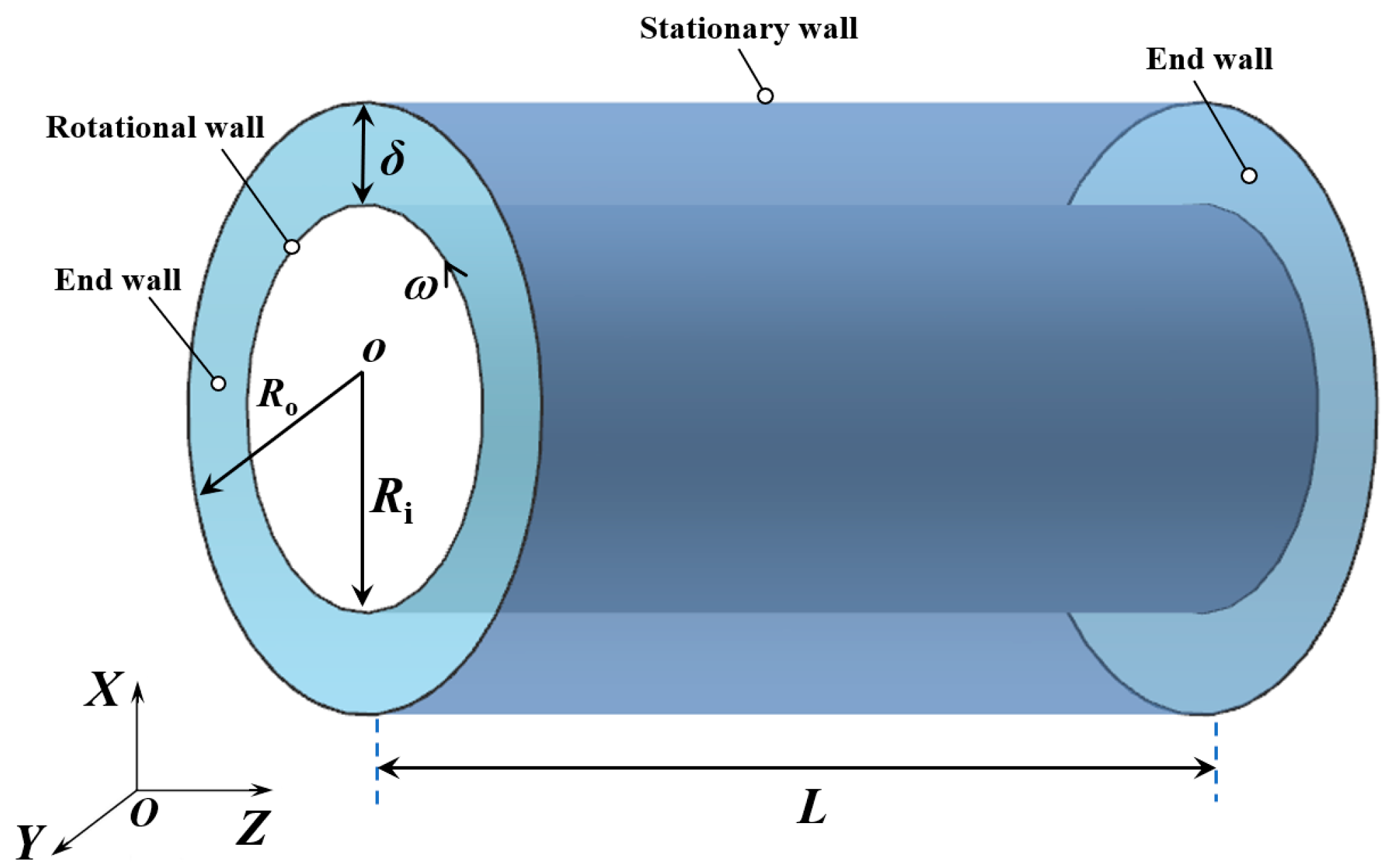
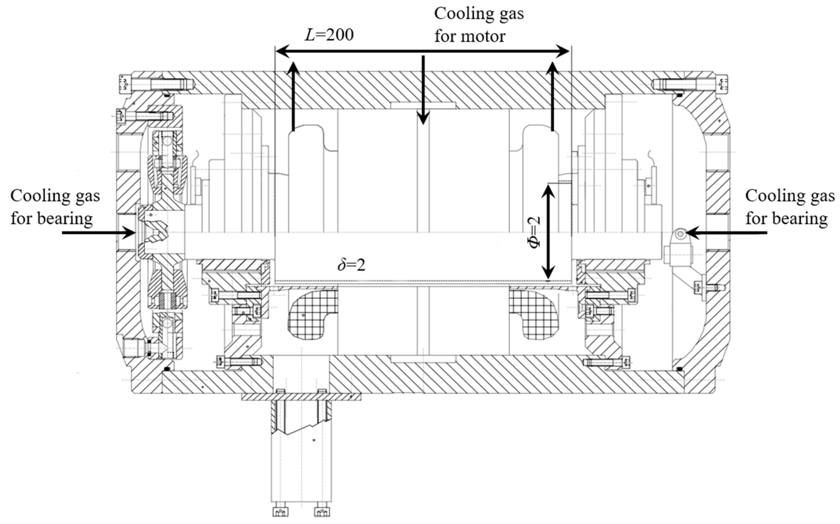
2.1. Geometric Model and Boundary Conditions

The computation domain shown in Figure 2, which is composed of two end walls, a rotational wall and a fixed wall, was adopted as the research object to investigate the skin friction coefficient and flow characteristics in a shaft-type gap with rough walls by performing a three-dimensional numerical technique in this study. The main dimensions of the computation domain are defined by the inner and outer radii of the gap, Ri and Ro, the axial length L, and the gap width δ = RoRi. Additionally, two dimensionless parameters, Reynolds number Re, which depends on the flow state, and radius ratio η, which is related to geometric dimensions, are defined to explore their influences on the skin friction coefficient and flow.
Re and η are defined as follows:
R e = ρ ω R i R o R i μ
η = R o R i R i
where ρ and μ are the density and dynamic viscosity of fluid, respectively; Ri and Ro are the inner and outer radii of the gap, respectively; and ω is the rotational speed.
For the geometric model, Ri and L were fixed at 35.5 and 200 mm, respectively, which was consistent with Saari’s experimental apparatus shown in Figure 3 [23]. In addition, the gap width δ ranged from 2 to 8 mm to investigate the effects of the radius ratio on the skin friction coefficient. Ro and η can be determined by Ri and δ. The dimensions of Ro, δ, and η from Case I to Case IV are listed in Table 1.
For each case, the rotational speed of the two end walls and the stationary wall was zero, and that of the rotational wall was changed so that Re ranged from 102 to 107. It needs to be pointed out that since the fluid velocity is relatively high for sCO2 power devices and the boundary conditions of the numerical validation have to keep consistent with Sarri’s experiment, heat transfer performance was not considered in this paper; thus, all walls were set as adiabatic. Based on the manufacturing accuracy of the turbomachinery, the influence of surface roughness Ra of 0.8, 3.2, and 6.3 μm on the skin friction coefficient and flow characteristics are discussed and analyzed in detail. Moreover, in order to ensure that the research range of the Reynolds number can apply to more operating conditions of sCO2 power devices, critical CO2 (higher density than sCO2) with a pressure and temperature of 7.38 MPa and 304.13 K, respectively, was selected as the working fluid from Case I to Case IV. According to the data from NIST REFPROP [28,29], the density and dynamic viscosity of critical CO2 are set to be 467.60 kg/m3 and 33.035 μPa·s. In addition, the gravity effect was considered to be negligeable due to its little influence on flow while the apparatus was laid horizontally.

2.2. Numerical Method

The commercial software ANSYS Fluent was used to conduct the computational fluid dynamic (CFD) simulations of windage loss and flow characteristics in the gap. The steady-state and three-dimensional Reynolds-averaged Navier–Stokes (RANS) equations [12,17,30,31] were solved, using the governing equations as follows [32]:
Continuity equation:
x i ρ u i = 0
Momentum equation:
x i ρ u i u j + x j P + 2 3 μ e u i x i x i μ e u i x j + u j x i = 0
Energy equation:
x i ρ u i H x i λ + C p μ t P r t T x i = 0
where u is the fluid velocity, x is the direction of coordinate system, P is the fluid pressure, μe is the effective viscosity, H is the total enthalpy, λ is the thermal conductivity, Cp is the heat capacity at constant pressure, μt is the turbulent viscosity, Prt is the turbulent Prandtl number, T is the fluid temperature, and i and j are index values.
In addition, the above three governing equations needed to be combined with the realizable k-ε turbulence model to characterize the turbulence flow in this study. The turbulence kinetic energy k and dissipation rate ε can be solved by the following two equations [33]:
x j ρ k u j = x j μ + μ t σ k k x j + G k + G b ρ ε Y M
x j ρ ε u j = x j μ + μ t σ ε ε x j + ρ ε C 1 S ρ C 2 ε 2 k + v ε + C 1 ε ε k C 3 ε G b
where σk = 1.0, σε = 1.2, Gk is the generation item due to the mean velocity gradients, Gb is the generation of buoyancy, YM is the ratio of the fluctuating dilatation to the overall dissipation rate, S is the modulus of the mean rate-of-strain tensor, and C2, C1ε, and C3ε are constants. Moreover, C1 can be obtained based on the following equation:
C 1 = max 0.43 ,   γ γ + 5 ,   γ = S k ε ,   S = 2 S ij S ij
In this study, the finite volume approach with the second-order upwind equation was adopted to discretize the RANS equations, and the pressure-based solver was used for numerical integration. The computation stability during simulation was estimated by monitoring the torque. When the torque of the stationary and rotational walls reached a stable value, and the torque difference between the two walls was less than 1% with additional iterations, the numerical results were considered “steady”. In addition, the solution was converged and reliable when the residual values of continuity, momentum, and energy equations were less than 10−8, 10−5, and 10−5, respectively. None of the simulations had stability or convergence problems, and every simulation was larger than 3000 iterations.

2.3. Windage Loss and Skin Friction Coefficient

The shaft-type windage loss can be estimated, presented in ref. [21], as follows:
W = C f π ρ R i 4 ω 3 L
where Cf is the skin friction coefficient.
When flow is laminar in the shaft-type gap, according to theoretical analysis, Cf is calculated as follows:
C f = 2 R e
When turbulent flow occurs, Cf is determined by experiments and CFD simulations due to unattainable theoretical determination. If windage loss W and the skin friction coefficient Cf are investigated by adopting numerical or experimental methods, the generated torque T and rotational speed ω are known, so windage loss can be expressed:
W = T ω
And Cf can be obtained by substituting Equation (11) into Equation (9):
C f = T π ρ R i 4 ω 2 L

2.4. Turbulence Model Validation

For turbulent flow, it is essential to choose a proper turbulence model to investigate the skin friction coefficient and flow. The three commonly used turbulence models, realizable k-ε, k-ω, and Reynolds stress model (RSM), are used to evaluate the reliability of the numerical simulation. The Cf obtained from Nakabayashi’s experiment was selected as the benchmark for the validation, and the device’s dimensions and experimental conditions used for verification are listed in Table 2 [26]. It needs to be noted that the inner wall was stationary and the rotational speed of outer wall depends on Re, which ranges from 103 to 3.7 × 10⁴. Moreover, the first cell height near the walls is varied to ensure that the maximum Y+ is in the range required by the turbulence models.
Figure 4 compares the numerical results using different turbulence models with Nakabayashi’s experimental data. It was found that the maximum relative deviation between the numerical results adopting the realizable k-ε model with enhanced wall treatment and the experimental data was only 8.7%, which was minimal compared to the other deviations. This indicated that selecting the realizable k-ε model with enhanced wall treatment to predict Cf and simulate the flow characteristics in a shaft-type gap with rough walls was appropriate. In addition, the enhanced wall treatment, which required that the maximum Y+ was close to 1, was used to resolve the flow characteristics in more detail within the boundary layer. Therefore, the realizable k-ε model with enhanced wall treatment was adopted to study turbulent flow. For laminar flow with Re < 103, the laminar model was selected as viscous mode.

2.5. Grid Independence Validation

The structured mesh and its partially enlarged detail shown in Figure 5 was generated using ANSYS ICEM. Since the flow was complex within boundary layer, the mesh was denser near the walls than at the center of the gap. Meanwhile, the first cell height of the walls was set at 5.0 × 10⁻⁵ mm, which ensured that the maximum Y+ near the walls was less than 1 and satisfied the requirements of the realizable k-ε model with enhanced wall treatment. Moreover, the maximum cell skewness was in the range of 0.06~0.1, indicating that the mesh quality was completely acceptable.
To avoid the impact of the number of grids on the numerical results and reduce the computing time, a grid independence validation was performed with four different meshes of 1.6 million, 3.2 million, 6.4 million, and 9.6 million grids aiming at the geometric model of Case I before the CFD simulations. The skin friction coefficient Cf under different Re is described in Figure 6 for each grid. It was found that Cf gradually remained approximately constant as the number of grids increased, and its maximum relative deviation was 0.49% when the number of grids increased from 6.4 million to 9.6 million. This indicated that 6.4 million grids could achieve a grid-independent solution.

3. Results and Discussion

In this section, the skin friction coefficient Cf and flow characteristics versus Reynolds number Re are analyzed, respectively, for Re of 102~107 and surface roughness Ra of 0.8~6.3 μm. In addition, the effects of the radius ratio η on Cf and flow characteristics are discussed under Ra = 0.8 μm conditions.

3.1. Effects of Reynolds Number and Surface Roughness on Skin Friction Coefficient

Figure 7 presents the skin friction coefficient Cf versus Re for the geometry of Case I when Ra ranged from 0 (smooth wall) to 6.3 μm, and the corresponding values are listed in Table 3. It was found that Cf decreased as Re increased for Re of 102~107. The rate of decrease was almost constant when Re was less than 103, but it gradually decreased with Re > 103, which resulted in Cf being independent of Re for values larger than 105. The conclusion was validated in the literature [5,25], according to Hu’s and Theodoresen’s studies.
It was found that the Cf of smooth walls was close to that of rough walls when Re < 4 × 10², but the difference between them was obvious when Re ≥ 4 × 10². The reason will be analyzed in Figure 8. In addition, the change trend of Cf was different at Ra = 0.8~6.3 μm in two ranges of Re, 102~105 and 105~107. When Re ≤ 105, the values of Cf were considerably close, indicating that Ra does not influence Cf at low Re. When Re > 105, it was noted that Cf gradually increased, but the rate of increase decreased when Ra increased from 0.8 to 6.3 μm; thus, the effects of Ra on Cf could not be ignored at high Re. This is because the flow at high Re was more easily influenced by rough walls than at low Re, resulting in larger Cf.
In order to estimate the effect of Ra on Cf, the relative deviation Δ between the skin friction coefficients of smooth and rough walls is defined as follows:
Δ = C f ,   r C f ,   s C f ,   s × 100 %
where Cf,s denotes Cf of rough walls and Cf,s denotes Cf of smooth walls.
Figure 8 presents the relative deviation versus Re under different Ra of 0.8~6.3 μm conditions. It was found that the relative deviations of 0.3%~0.6% for Re = 102 were far smaller than those when Re ranged from 103 to 107. This indicated that the Cf of rough walls was the same as that of smooth walls for extremely low Re, which was consistent with the conclusion drawn in Figure 7. However, when Re > 102, the relative deviations rapidly increased with increasing Re and Ra, attaining a maximum of 203% at Re = 107 and Ra = 6.3 μm, indicating that Cf was influenced by both flow and wall roughness. This is because at low Re, the flow in the gap was laminar and the boundary layer was relatively thick, which means the grain of the rough walls was completely covered by the viscous sublayer for Ra = 0.8~6.3 μm; thus, Cf and flow were little influenced by rough walls. However, with increasing Re or Ra, the boundary layer became thinner, and the grain was in blending or there were logarithmic law regions even outside boundary layer, which significantly impacted the flow near the walls or at the center of the gap, resulting in increased Cf.

3.2. Effects of Reynolds Number and Surface Roughness on Flow Characteristics

The flow characteristics will be discussed in this subsection to analyze the reasons that Cf is influenced by Re and Ra. Figure 9 shows the streamlines and velocity magnitude at the meridional plane with Re of 102, 104, and 107 for Ra = 0.8~6.3 μm. It is worth mentioning that since the flow was highly similar at the axial direction in the whole gap, Figure 9 only shows the contours near one end wall.
When Re = 102, it can be seen that the streamlines were considerably similar than when Ra ranged from 0.8 to 6.3 μm, which further validated that Ra does not influence the flow in the gap and leads to Cf being highly close for different values of Ra, as shown in Figure 7 and Figure 8. Moreover, except for the vortex near the end wall, which is due to the combined effect of the boundary layer of all walls, including the two end walls, the flow in whole gap was laminar and no vortexes occurred. Under Re = 104 and Re = 107 conditions, it can be seen that the flow transitioned from laminar flow to TC flow and periodic Taylor vortexes appeared, the number of which increased with Ra, resulting in increased Cf, as described in Figure 7. Additionally, when Re ≥ 104, the size of the Taylor vortexes increased as Re increased. This is because a higher Re reflected a higher rotational speed and greater centrifugal force was applied to the fluid, leading to more complex and unstable flow.
In addition, it was found that the velocity was higher near the inner walls under higher Re conditions, and it decreased to zero near the outer walls along the radial direction. The reason is that a higher Re indicated a higher rotational speed, combined with the no-slip wall conditions, which resulted in the fluid velocity near the walls being the same as the linear velocity of the walls. To analyze the velocity distribution in the gap in more detail, Figure 10 presents the velocity in the radial direction with Re = 104 and Ra = 0.8~6.3 μm.
According to Figure 10, the velocity was divided into three regions. Moreover, the fluid velocity in the speed-stable region that increased with Ra was approximately half of the inner walls’ linear speed, which was consistent with the velocity distribution shown in Figure 9. In addition, the velocity gradient in the speed-drop regions, which also increased with Ra, was significantly larger than that in the speed-stable region. These results indicated that Ra influenced the thickness of the boundary layer and flow near the walls, but the flow in the center of the gap was more stable.

3.3. Effects of Radius Ratio on Skin Friction Coefficient and Flow Characteristics

Figure 11 describes the skin friction coefficient Cf versus Re for the radius ratio η ranging from 0.056 to 0.225, corresponding to the geometric model from Case I to Case IV, at Ra = 0.8 μm. The values of Cf are listed in Table 4. Similar to Figure 7, Cf gradually decreased when Re increased from 102 to 107 for all cases. The rate of decrease versus Re was constant when Re < 103, but it slowly decreased when Re ≥ 103, which led to Cf remaining constant for Re > 105. In addition, it was also found that Cf and the variation rate increased with η, which indicated that Cf was seriously influenced by larger η. The reason is that the TC flow was prominent and more Tarloy vortexes occurred at larger η, resulting in increased Cf.
According to Equation (13), the relative deviations at η = 0.056~0.225 were calculated and are shown in Figure 12. It was found that the relative deviations increased with Re and η when Re ≤ 105, but they decreased with Re and increasing η for Re > 105. This indicated that Cf was more easily influenced by rough walls for larger η under lower Re conditions, but the opposite occurred for significantly higher Re. This is because the flow was stable at low Re, and the interaction between rough walls and working fluid influenced windage loss; hence, it was more prominent in a larger gap width, corresponding to a larger η. However, the flow was extremely unstable at high Re and became the primary source of windage loss; hence, in a smaller gap width, meaning a smaller η, the flow was more significantly impacted by rough walls, resulting in larger relative deviations. Additionally, when Re = 102, the fact that the relative deviations ranged from 0.6% to 2.9% also indicated that the Cf of rough walls was similar to that of smooth walls for extremely low Re, as shown in Figure 8.
Figure 13 shows the streamlines and vorticity contours near one end wall at the meridional plane with Re of 102, 104, and 107 at η = 0.056~0.225. It can be seen that no Taylor vortexes occurred when Re = 102 for each case, which indicated that the flow was not impacted by rough walls no matter how wide the gap. This was also the most crucial reason that the Cf of rough walls was almost the same as that of smooth walls, as shown in Figure 13. When Re was equal to 104 and 107, the size of Taylor vortexes increased with η, automatically leading to fewer vortexes. This was because a larger η means a larger gap width, resulting in Taylor vortexes forming more easily and developing in the gap. Further, it was noted that the size of vortexes near the end wall increased as Re increased, indicating that the effect of the end walls was more permanent for higher Re.
Moreover, it was also found that when Re = 102, the vorticity distribution was near the end walls and it increased with η. The reason was that the centrifugal force exerted on the fluid in the gap was exceedingly small at lower Re, so the effect of the stationary end walls could not be ignored; thus, the effect of the end walls was more prominent under larger η and gap width conditions. However, the centrifugal force was larger for higher Re; hence the impact of the end walls was not significant, which resulted in the vorticity near the end wall decreasing as η increased, as shown in the vorticity contours for Re of 104 and 107. Further, it can be seen that the vorticity in the whole gap increased with Re for all cases, indicating that the dissipated energy due to the vortexes was greater at higher Re.
Figure 14 shows the pressure contours in the tangential direction and velocity distribution in the radial direction when Re was 104. It is noted that the pressure P in the legends is 7.38 MPa, which is critical CO2 pressure.
It was found that the pressure gradually increased from the rotational to stationary walls according to the law of energy conservation, which corresponded to the velocity distribution shown in Figure 9, but it decreased with increasing η as a whole. Additionally, there were periodic low-pressure and high-pressure regions near the walls as a result of Taylor vortexes in the gap, and the periodic high-pressure regions near the stationary walls decreased at larger η. This was because when η increased, the size of the Taylor vortexes increased but fewer vortexes occurred; hence the periodic fluctuation of pressure was less, resulting in fewer high-pressure regions. Moreover, it was noted that the velocity distribution was similar to Figure 10 for different cases, which could also be divided into three regions, but the velocity gradient near the stationary walls for Case IV was smaller than that of other Cases due to the significantly larger η.

4. Conclusions

To investigate the influence of surface roughness on windage loss and flow in the shaft-type gap of generators, the skin friction coefficient Cf and flow characteristics versus Reynolds number Re were analyzed for different surface roughness Ra, and the effects of radius ratio η were discussed under Ra of 0.8 μm conditions. The conclusions of this paper will help develop a model for predicting Cf with rough walls, further improving the design of small supercritical carbon dioxide power devices, including turbine-alternator-compressor units. The main conclusions are as follows:
(1)
Cf decreased as Re increased, and the rate of decrease was constant at low Re but it gradually decreased at high Re. In addition, for Re = 102, the relative deviations between the skin friction coefficients of smooth and rough walls of 0.3~0.6% indicated that Cf was not influenced by rough walls. However, when Re > 102, the relative deviations increased with Re and Ra, indicating that Cf was influenced by flow and rough walls because the grain was in blending or logarithmic law regions occurred, which impacted the flow.
(2)
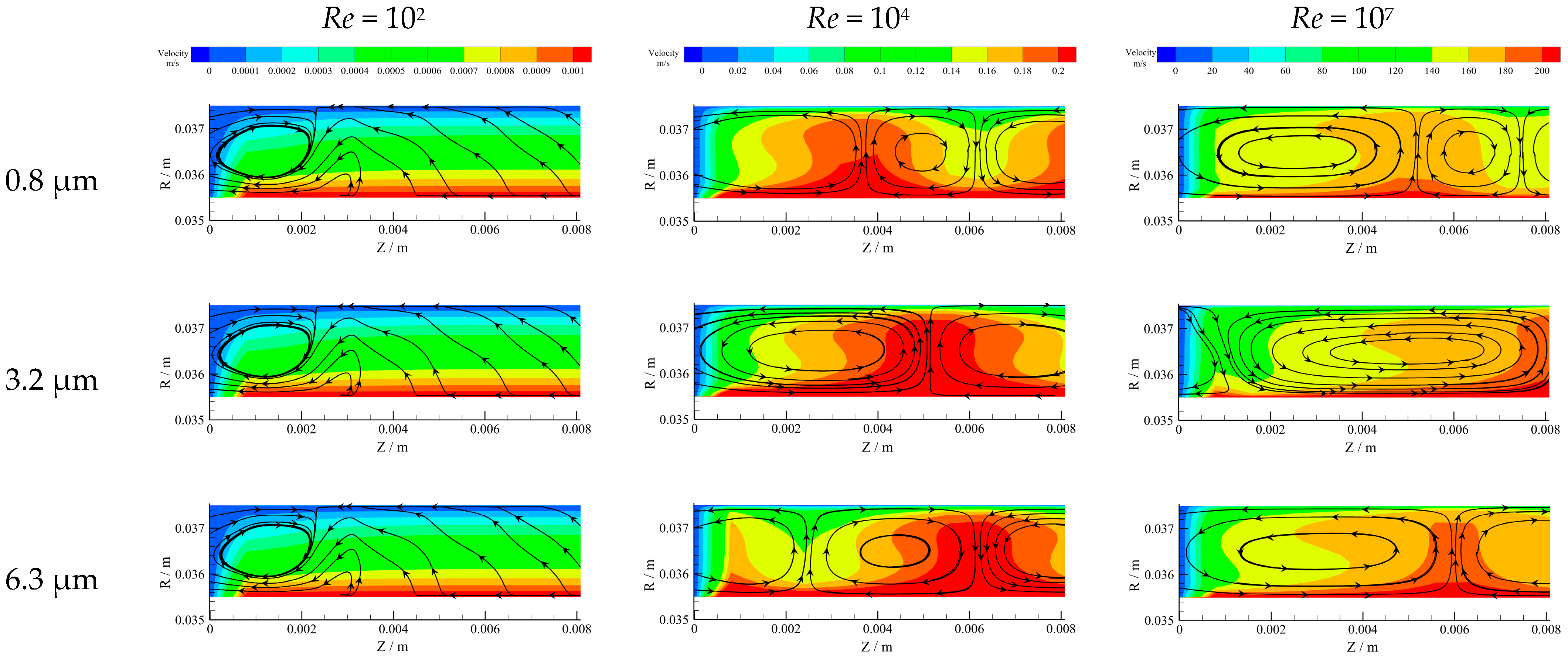
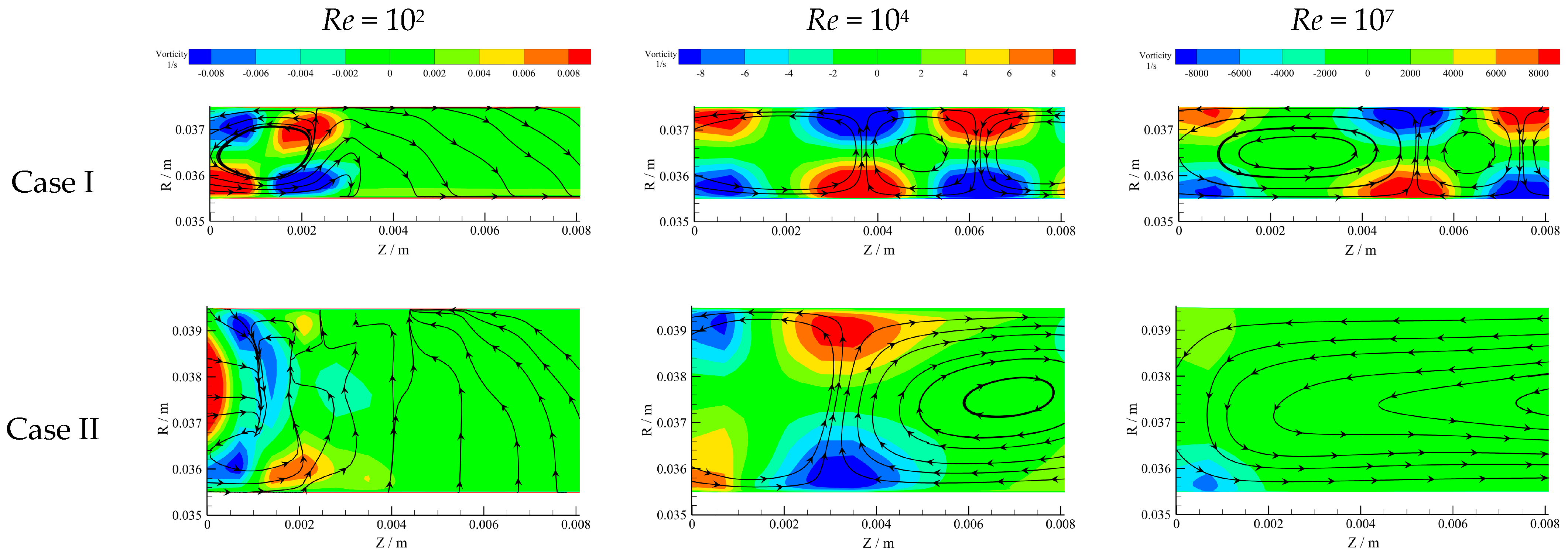
When Re = 102, the flow was laminar and similar for different Ra, but when Re > 102, it transitioned to TC flow and periodic Taylor vortexes appeared, the number of which increased with Ra. The velocity could be divided into three regions, and the speed-stable region increased with Ra. The velocity gradient in speed-drop regions was larger than that in speed-stable regions. These results indicated that Ra influenced the thickness of the boundary layer and the flow at the center of the gap was more stable.
(3)
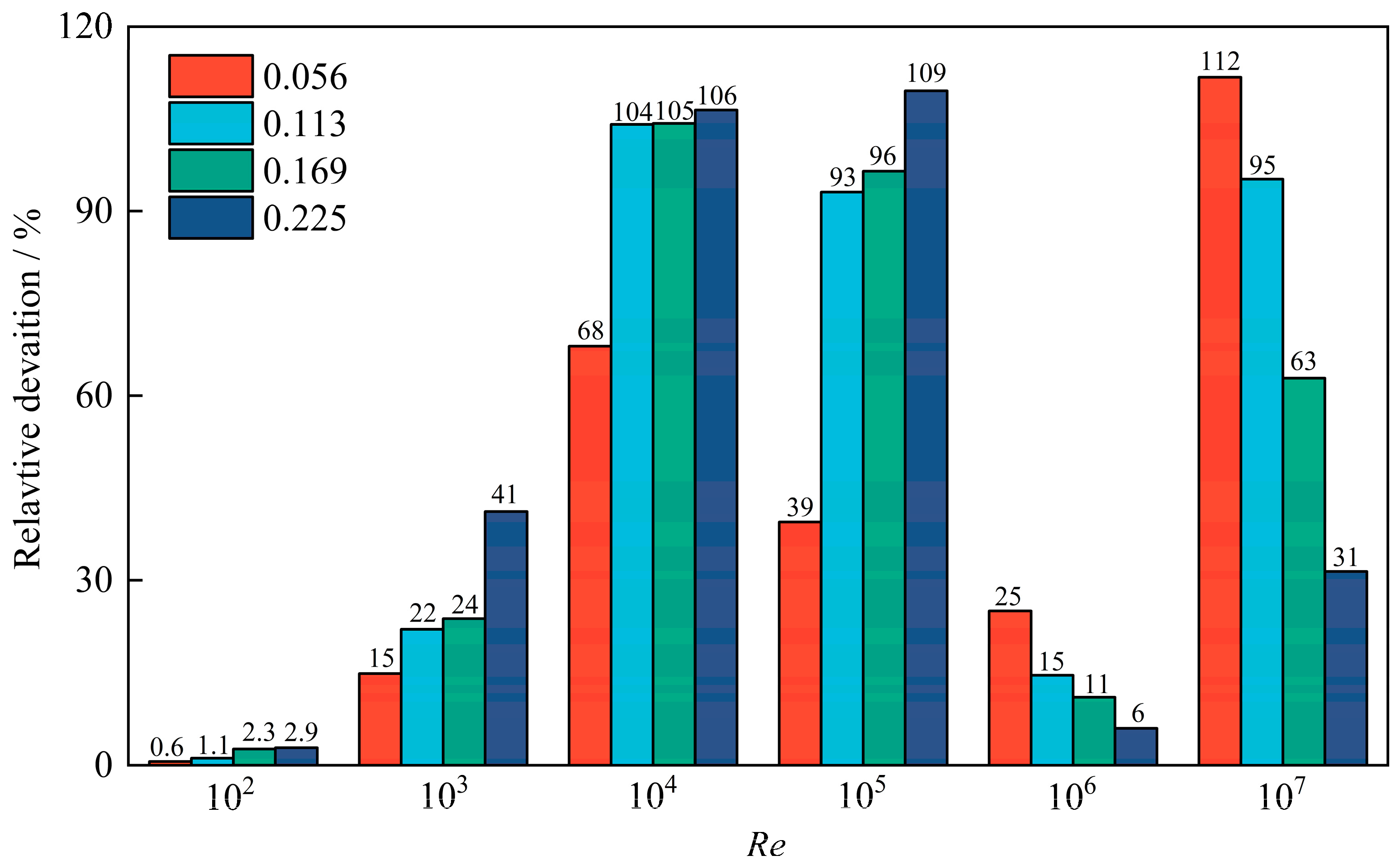
Cf and the variation rate increased with η, indicating the Cf was seriously influenced by larger η. Moreover, the relative deviations increased with η when Re ≤ 105, which indicated that Cf was more easily influenced by rough walls for larger η under low Re conditions, since the interaction between rough walls and working fluid affected windage loss. However, the opposite was true when Re > 105 because the flow became the primary source of windage loss in a smaller gap width at high Re.
(4)
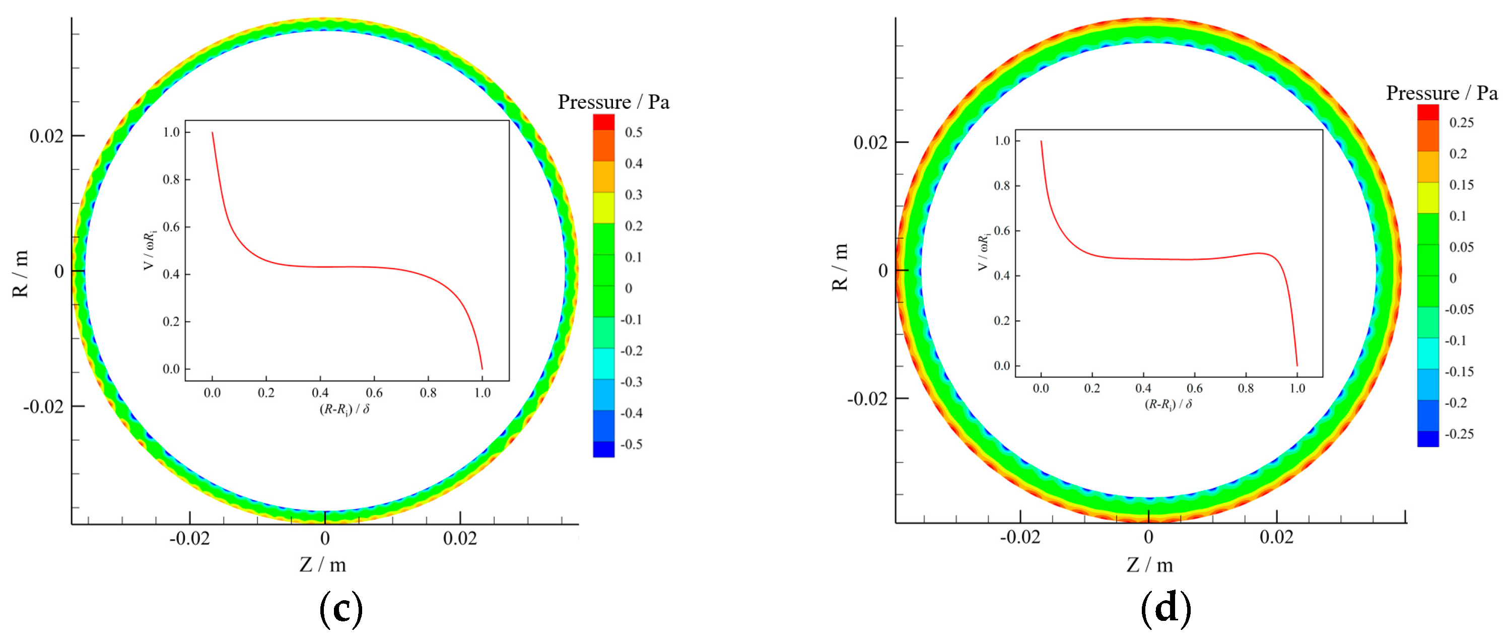
The size of Taylor vortexes increased with η, leading to fewer vortexes. In addition, the pressure gradually increased from the rotational to stationary walls but decreased with increasing η as a whole. Additionally, there were periodic low-pressure and high-pressure regions near the walls due to Taylor vortexes in the gap, but the periodic high-pressure regions near the stationary walls decreased at larger η, since the number of Taylor vortexes decreased. Moreover, the velocity gradient near the stationary walls for Case IV was smaller than that of other Cases due to the significantly large η.

Author Contributions

Methodology, L.H.; software, L.H.; data curation, Q.D. and J.L.; writing—original draft preparation, L.H.; writing—review and editing, Q.D. and Z.F.; visualization, Z.L.; supervision, Q.D.; funding acquisition, Q.D. All authors have read and agreed to the published version of the manuscript.

Funding

This work was supported by the Joint Funds of the National Natural Science Foundation of China (U20A20303) and the National Key R&D Program of China (2017YFB0601804).

Institutional Review Board Statement

Not applicable.

Informed Consent Statement

Not applicable.

Data Availability Statement

Data will be made available on request.

Acknowledgments

We acknowledge the support and internal funding from the Joint Funds of the National Natural Science Foundation of China (U20A20303) and the National Key R&D Program of China (2017YFB0601804).

Conflicts of Interest

The authors declared no conflict of interest.

References

  1. Xu, J.; Sun, E.; Li, M.; Liu, H.; Zhu, B. Key issues and solution strategies for supercritical carbon dioxide coal fired power plant. Energy 2018, 157, 227–246. [Google Scholar] [CrossRef]
  2. Sathish, S.; Kumar, P. Equation of state based analytical formulation for optimization of sCO2 Brayton cycle. J. Supercrit. Fluids. 2021, 177, 105351. [Google Scholar] [CrossRef]
  3. Xue, J.; Nie, X.; Zhao, L.; Zhao, R.; Wang, J.; Yang, C.; Lin, A. Molecular dynamics investigation on shear viscosity of the mixed working fluid for supercritical CO2 Brayton cycle. J. Supercrit. Fluids 2022, 182, 105533. [Google Scholar] [CrossRef]
  4. Cao, R.; Li, Z.; Deng, Q.; Li, J. Design and aerodynamic performance investigations of supercritical carbon dioxide centrifugal compressor. In Proceedings of the ASME Turbo Expo, American Society of Mechanical Engineers (ASME), Virtual, 21–25 September 2020. [Google Scholar] [CrossRef]
  5. Hu, L.; Deng, Q.; Li, J.; Feng, Z. Model improvement for shaft-type windage loss with CO2. J. Supercrit. Fluids. 2022, 190, 105747. [Google Scholar] [CrossRef]
  6. Fleming, D.; Conboy, T.; Pash, J.; Rochau, G.; Fuller, R.; Holschuh, T.; Wright, S. Scaling Considerations for a Multi-Megawatt Class Supercritical CO2 Brayton Cycle and Commercialization; Sandia National Laboratory: Albuquerque, NM, USA, 2013.
  7. Wright, S. Summary of the Sandia Supercritical CO2 Development Program; Sandia National Laboratory: Albuquerque, NM, USA, 2011.
  8. Quiban, R.; Changenet, C.; Marchesse, Y.; Ville, F. Experimental investigations about the power loss transition between churning and windage for spur gears. J. Tribol. 2020, 143, 024501. [Google Scholar] [CrossRef]
  9. Zhao, Z.; Song, W.; Jin, Y.; Lu, J. Effect of rotational speed variation on the flow characteristics in the rotor-stator system cavity. Appl. Sci. 2021, 11, 11000. [Google Scholar] [CrossRef]
  10. Shen, G.; Yao, J.; Lou, W.; Chen, Y.; Guo, Y.; Xing, Y. An experimental investigation of streamwise and vertical wind fields on a typical three-dimensional hill. Appl. Sci. 2020, 10, 1463. [Google Scholar] [CrossRef] [Green Version]
  11. Conboy, T.; Wright, S.; Pasch, J.; Fleming, D.; Rochau, D.; Fuller, R. Performance characteristics of an operating supercritical CO2 Brayton cycle. J. Eng. Gas Turbines Power. 2012, 134, 111703. [Google Scholar] [CrossRef]
  12. Anderson, K.; Lin, J.; Namara, M.; Magri, V. CFD study of forced air cooling and windage losses in a high speed electric motor. J. Electron. Cool. Therm. Control. 2015, 5, 27–44. [Google Scholar] [CrossRef]
  13. Asami, F.; Miyatake, M.; Yoshimoto, S.; Tanaka, E.; Yamauchi, T. A method of reducing windage power loss of a high-speed motor using a viscous vacuum pump. Precis. Eng. 2017, 48, 60–66. [Google Scholar] [CrossRef]
  14. Kiyota, K.; Kakishima, T.; Chiba, A. Estimation and comparison of the windage loss of a 60 kW switched reluctance motor for hybrid electric vehicles. In Proceedings of the 2014 International Power Electronics Conference, Hiroshima, Japan, 18–21 May 2014. [Google Scholar] [CrossRef]
  15. Liu, M.; Sixel, W.; Ding, H.; Sarlioglu, B. Investigation of rotor structure influence on the windage loss and efficiency of FSPM machine. In Proceedings of the 2018 IEEE Energy Conversion Congress and Exposition, Portland, OR, USA, 23–27 September 2018. [Google Scholar] [CrossRef]
  16. Sun, D.; Zhou, M.; Zhao, H.; Liu, J.; Fei, C.; Li, H. Numerical and experimental investigations on windage heating effect of labyrinth seals. J. Aerosp. Eng. 2020, 33, 04020057. [Google Scholar] [CrossRef]
  17. Nachouane, A.; Abdelli, A.; Friedrich, G.; Vivier, S. Estimation of windage losses inside very narrow air gaps of high speed electrical machines without an internal ventilation using CFD methods. In Proceedings of the 2016 International Conference on Electrical Machines, Lausanne, Switzerland, 4–7 September 2016. [Google Scholar] [CrossRef]
  18. Wendt, V. Turbulente strmungen zwischen zwei rotierenden konaxialen zylinder. Ingenieur-Archiv 1933, 4, 577–595. [Google Scholar] [CrossRef]
  19. Bilgen, E.; Boulos, R. Functional dependence of torque coefficient of coaxial cylinders on gap width and Reynolds numbers. J. Fluid. Eng. 1973, 95, 122–126. [Google Scholar] [CrossRef]
  20. Yamada, Y. Torque resistance of a flow between rotating co-axial cylinders having axial flow. Bull. JSME 1962, 186, 634–642. [Google Scholar] [CrossRef] [Green Version]
  21. Vrancik, J. Prediction of Windage Power Loss in Alternators; NASA: Washington, DC, USA, 1968.
  22. Deng, Q.; Hu, L.; Zhao, Y.; Yang, G.; Li, J.; Feng, Z. Verification of windage loss model and flow characteristic analysis in shaft-type gap. J. Xi’an Jiaotong. Univ. 2022, 56, 57–66. [Google Scholar] [CrossRef]
  23. Sarri, J. Thermal Analysis of High-Speed Induction Machines; Helsinki University of Technology: Espoo, Finland, 1998. [Google Scholar]
  24. Hu, L.; Deng, Q.; Zhao, Z.; Li, J.; Feng, Z. Flow characteristics and windage loss of CO2 in shaft-type rotor-stator gap. J. Eng. Thermophys. 2022, 43, 647–655. [Google Scholar]
  25. Theodorsen, T.; Regier, A. Experiments on Drag of Revolving Disks, Cylinders, and Streamline Rods at High Speeds; NACA: Boston, MA, USA, 1944.
  26. Nakabayashi, K.; Yamada, Y.; Kishimoto, T. Viscous frictional torque in the flow between two concentric rotating rough cylinders. J. Fluid Mech. 1982, 119, 409–422. [Google Scholar] [CrossRef]
  27. Rasmussen, E.; Yellapantula, S.; Martin, M. How equation of state selection impacts accuracy near the critical point: Forced convection supercritical CO2 flow over a cylinder. J. Supercrit. Fluids 2021, 171, 105141. [Google Scholar] [CrossRef]
  28. NIST Standard Reference Database 23. NIST Thermodynamic and Transport Properties of Refrigerants and Refrigerant Mixtures-REFPROP; Version 6.01; National Institute of Standards and Technology: Gaithersburg, MD, USA, 1998. [Google Scholar]
  29. Span, R.; Wagner, W. A new equation of state for carbon dioxide covering the fluid region from the triple point temperature to 1100 K at pressures up to 800 MPa. Phys. Chem. Ref. Data 1996, 25, 1509–1596. [Google Scholar] [CrossRef] [Green Version]
  30. Qin, K.; Li, D.; Huang, C.; Sun, Y.; Wang, J.; Luo, K. Numerical investigation on heat transfer characteristics of Taylor Couette flows operating with CO2. Appl. Therm. Eng. 2020, 163, 114570. [Google Scholar] [CrossRef]
  31. Adebayo, D.; Rona, A. Numerical investigation of the three-dimensional pressure distribution in Taylor Couette flow. J. Fluids Eng. 2017, 139, 111201. [Google Scholar] [CrossRef]
  32. Tao, W. Numerical Heat Transfer, 2nd ed.; Xi’an Jiaotong University Press: Xi’an, China, 2010. [Google Scholar]
  33. ANSYS. ANSYS Fluent Theory Guide 2020 R2; ANSYS Inc.: Canonsburg, PA, USA, 2020. [Google Scholar]
Figure 1. Meridian plane of a turbine-alternator-compressor (TAC) unit.
Applsci 12 12631 g001
Figure 2. Schematic diagram of computational domain composed of two end walls, a rotational wall and a fixed wall.
Applsci 12 12631 g002
Figure 3. Schematic diagram of Saari’s experimental apparatus [23].
Applsci 12 12631 g003
Figure 4. Comparison of numerical results for three turbulence models and Nakabayashi’s experimental data.
Applsci 12 12631 g004
Figure 5. Structured mesh of computational domain and its partially enlarged detail.
Applsci 12 12631 g005
Figure 6. Skin friction coefficient Cf under different Re for four different meshes of 1.6 million, 3.2 million, 6.4 million, and 9.6 million grids.
Applsci 12 12631 g006
Figure 7. Skin friction coefficient Cf versus Re for the geometry of Case I when Ra ranges from 0 (smooth wall) to 6.3 μm.
Applsci 12 12631 g007
Figure 8. Relative deviation versus Re under Ra of 0.8~6.3 μm conditions.
Applsci 12 12631 g008
Figure 9. Streamlines and velocity magnitude at meridional plane with Re of 102, 104, and 107 for Ra, Ra = 0.8~6.3 μm.
Applsci 12 12631 g009
Figure 10. Averaged velocity in the radial direction with Re = 104 and Ra = 0.8~6.3 μm.
Applsci 12 12631 g010
Figure 11. Skin friction coefficient Cf versus Re for η ranging from 0.056 to 0.225 at Ra = 0.8 μm.
Applsci 12 12631 g011
Figure 12. Relative deviations versus Re under η = 0.056~0.225 conditions.
Applsci 12 12631 g012
Figure 13. Streamlines and vorticity contours at meridional plane with Re of 102, 104, and 107 at different η = 0.056~0.225.
Applsci 12 12631 g013aApplsci 12 12631 g013b
Figure 14. Pressure contours in the tangential direction and velocity distribution in the radial direction for Re = 104 (a) Case I; (b) Case II; (c) Case III; (d) Case IV.
Applsci 12 12631 g014aApplsci 12 12631 g014b
Table 1. Dimensions of outer radius Ro, gap width δ, and radius ratio η.
DescriptionCase ICase IICase IIICase IVUnit
Outer radius Ro37.539.541.543.5mm
Gap width δ2468mm
Radius ratio η0.0560.1130.1690.225
Table 2. Device’s dimensions and experimental conditions used for turbulence model validation.
DescriptionValueUnit
Inner radius Ri30.7mm
Outer radius Ro33.6mm
Gap width δ2.9mm
Axial length L90mm
Surface roughness Ra0.211mm
Table 3. Values of Cf at different Re when Ra ranges from 0 (smooth wall) to 6.3 μm for Case I.
ReRa/mmCf
10202.69 × 10−2
0.82.70 × 10−2
3.22.70 × 10−2
6.32.69 × 10−2
10306.92 × 10−3
0.87.96 × 10−3
3.27.88 × 10−3
6.37.88 × 10−3
10402.19 × 10−3
0.83.68 × 10−3
3.23.72 × 10−3
6.33.74 × 10−3
10501.26 × 10−3
0.81.39 × 10−3
3.21.54 × 10−3
6.31.75 × 10−3
10607.55 × 10−4
0.89.44 × 10−4
3.21.31 × 10−3
6.31.52 × 10−3
10704.30 × 10−4
0.89.11 × 10−4
3.21.16 × 10−3
6.31.30 × 10−3
Table 4. Values of Cf versus Re for η ranging from 0.056 to 0.225 at Ra = 0.8 μm.
ReRa/mmCf
1020.0562.70 × 10−2
0.1134.93 × 10−2
0.1698.47 × 10−2
0.2251.49 × 10−1
1030.0567.96 × 10−3
0.1139.11 × 10−3
0.1691.09 × 10−2
0.2251.56 × 10−2
1040.0563.68 × 10−3
0.1134.55 × 10−3
0.1695.16 × 10−3
0.2255.49 × 10−3
1050.0561.39 × 10−3
0.1132.35 × 10−3
0.1692.54 × 10−3
0.2252.68 × 10−3
1060.0569.44 × 10−4
0.1131.19 × 10−3
0.1691.50 × 10−3
0.2251.71 × 10−3
1070.0569.11 × 10−4
0.1139.51 × 10−4
0.1691.29 × 10−3
0.2251.49 × 10−3
Publisher’s Note: MDPI stays neutral with regard to jurisdictional claims in published maps and institutional affiliations.

