Article

Mathematical Models of Grinding Forces in the Hob Cutter Sharpening Process

by
Błażej Witkowski
,
Wojciech Stachurski
,
Witold Pawłowski
,
Małgorzata Sikora
and
Norbert Kępczak
*
Institute of Machine Tools and Production Engineering, Faculty of Mechanical Engineering, Lodz University of Technology, Stefanowskiego 1/15, 90-537 Lodz, Poland
*
Author to whom correspondence should be addressed.
Materials 2025, 18(1), 138; https://doi.org/10.3390/ma18010138
Submission received: 8 December 2024 / Revised: 30 December 2024 / Accepted: 30 December 2024 / Published: 1 January 2025

Abstract

:
The article presents the results of research aimed at developing mathematical models for determining the components of grinding force occurring during the sharpening of the rake face of hob cutters. The development of the models was based on the results obtained during experimental tests conducted in the first stage of the research. The studies were carried out using a tool grinder and an aluminum oxide grinding wheel. During the tests, two components of the grinding force were measured, using a piezoelectric dynamometer. A sample made of HS6-5-2 high-speed steel was ground. Grinding was carried out using different sets of cutting parameters. Based on the obtained measurement results, two mathematical models were developed in the form of (1) a multiple regression function and (2) a polynomial function, enabling the calculation of the normal and the tangential force. The experimentally obtained results were then compared with those calculated based on the developed models, and the results of this comparison showed that the developed models provide a good basis for analyzing the sharpening process of hob cutters in terms of variable grinding parameters.

1. Introduction

In the era of mass industrial production of gears [1], the proper regeneration of hob cutters, cutting tools commonly used for manufacturing toothed elements, is of great importance [2]. This is because improperly selected grinding conditions during the sharpening of the rake surfaces of the cutters can adversely affect the technological properties of the surface layer, causing, among other things, high thermal stresses leading to a network of cracks [3,4], and structural changes significantly reducing the cutting properties of the edges [5] and deteriorating their operational properties [6].
Therefore, it is extremely important to consciously shape the surface layer during grinding. The means to achieve this is to assess the course of the machining process, and one of the most important elements allowing for such an assessment is the knowledge of cutting forces. The significance of such an assessment lies in the dependence of the adjustable machining values, such as grinding parameters, the geometry of the contact between the grinding wheel and the workpiece, the characteristics of the grinding wheel, and the material properties on the values of the occurring forces. Moreover, knowledge of the obtained values of the grinding force components allows, among other things, for the determination of the grinding force coefficient μ, which provides information about the grinding efficiency [7], and the calculation of the total grinding power P, enabling the determination of the grinding index Ks [8]. Generally, the grinding force is considered a key indicator of the material removal process, which directly affects the machining efficiency, the quality of the machined surface, and the durability of the grinding wheel [9].
In a broader perspective, the values of the grinding force components obtained experimentally allow for the creation of mathematical models, and the force model is the simplest and most versatile mathematical expression describing the mechanical behaviour of material removal [9]. As shown by the comparative analysis presented in the study [9], mathematical models of the grinding force can come from various sources, including experimental data, empirical formulas, or theoretical analyses. It should be remembered that modelling the grinding force is a complex process, and the factors influencing the magnitude of the grinding force can include the physical properties of the machined material, the shape, size, and number of abrasive grains, grinding parameters, cooling and lubrication conditions, and the type of grinding process [10,11,12].
It is worth noting that grinding force models can be used in further research to model the dynamic grinding process. An example of such use is the model of the external plunge grinding process [13,14,15], the process of longitudinal cylindrical external grinding [16], and the process of peripheral surface grinding [17].
Therefore, this article presents research work, as a result of which two mathematical models were determined to predict the components of the grinding force during the sharpening of the rake surfaces of hob cutters. The research began with experimental studies, the conditions and methodology of which, as well as the results, are described in Section 2 and Section 3, respectively. The first of the two mathematical models presented in Section 4 is a modification of the model proposed by Werner [18]. It is worth noting that this model is often used, also with appropriate modifications, by other researchers [12,19,20]. The second mathematical model in the form of a multiple regression function was determined on the basis of algorithm of the “acceptance and rejection” method [21]. In the final part of the work, a comparison of the results obtained based on calculations using the proposed mathematical models with the results obtained experimentally was made. The work concludes with a summary and conclusions.

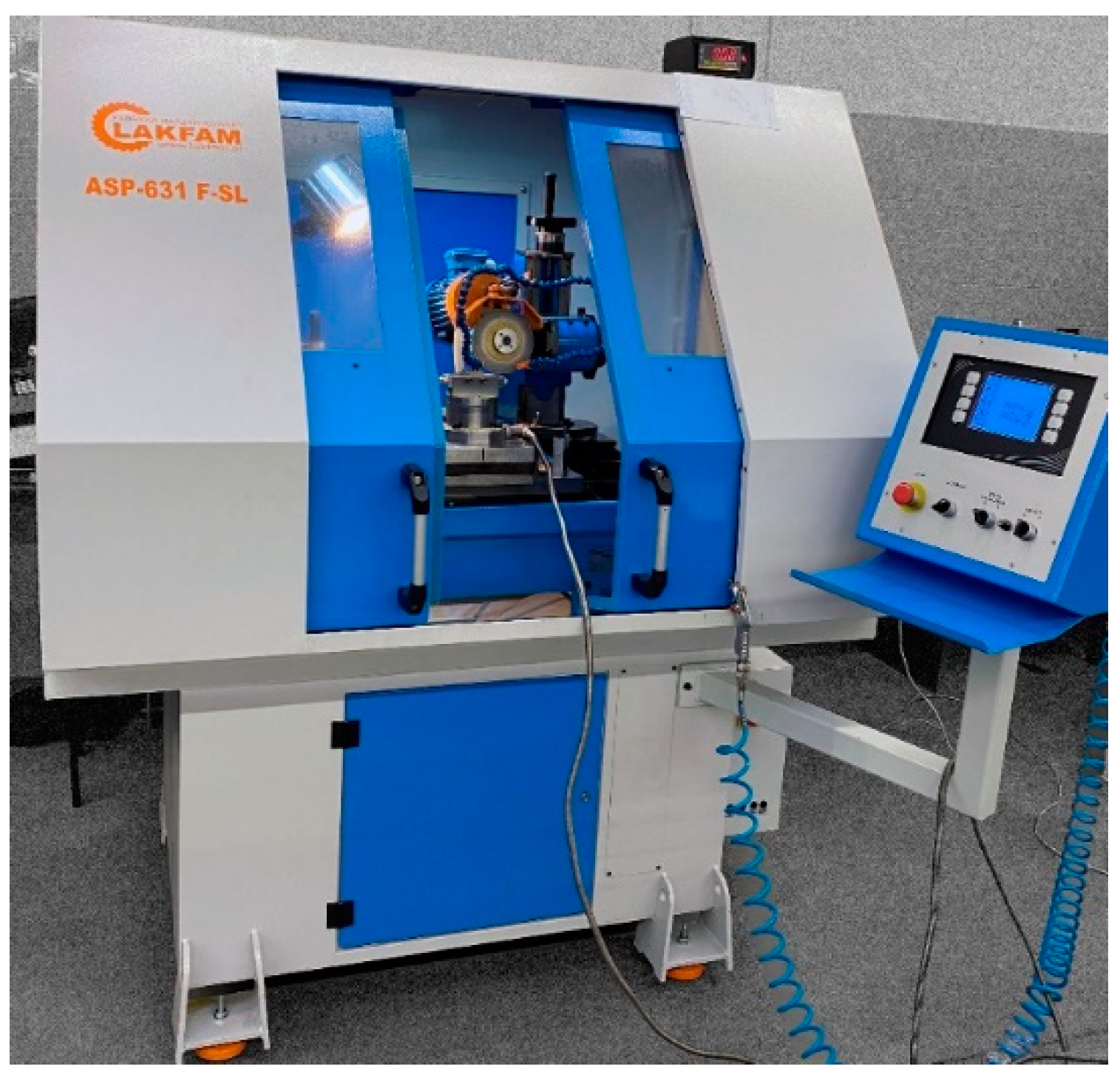
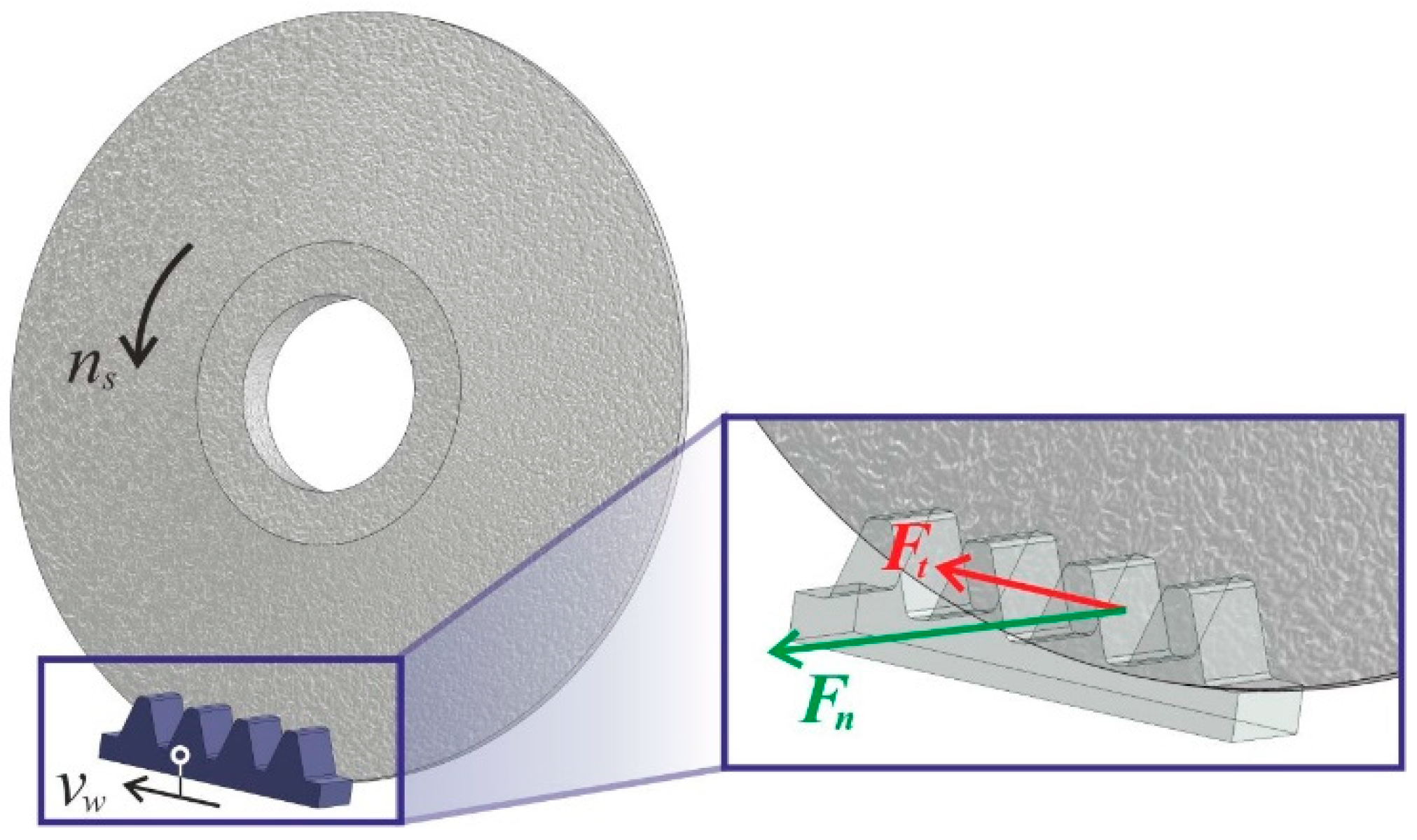
2. The Conditions and Methodology of the Research

The experimental studies were conducted on the ASP-631 F-SL tool grinder (Lakfam, Kowary, Poland), a general view of which is shown in Figure 1. The ASP-631 F-SL is a numerically controlled grinder in three axes for the automatic grinding of cutting tools along straight and helical lines. As such, it can be used for sharpening the rake surfaces of hob cutters.
In Figure 2, the workspace of the ASP-631 F-SL tool grinder is shown. As can be observed, a 4-component piezoelectric dynamometer type 9272 (Kistler, Winterthur, Switzerland) is mounted on the grinder table, previously separated from the table by a layer of insulator. The dynamometer was used to measure the components of the grinding force—the normal component Fn and the tangential component Ft. The signal from the dynamometer was transmitted to a four-channel amplifier Kistler type 5019A, then to the data acquisition card type KUSB-3108 (Keithley Instruments, Cleveland, OH, USA), which was finally connected to a PC. The Keithley quick DAQ software (version 1.6) was used to record the measurement signal.
A special holder for mounting the sample was attached to the upper surface of the dynamometer. During the tests, a sample made of high-speed steel HS6-5-2 with a hardness of 62 ± 1 HRC was ground. The shape of the sample in the part subjected to grinding had the outline of a gear, with dimensions corresponding to the dimensions of the cutting edge gear of a hob cutter with a module m = 3 mm and a pressure angle α = 20°, in accordance with ISO 53 and ISO 54. The geometric dimensions of the gear were selected according to PN 4468, taking into account the accuracy of the hob cutter edge in class B.
As the cutting tool, a T3 type grinding wheel with dimensions (D × T × H) 125 × 9/2 × 32 mm was used. The parameter D denotes the outer diameter of the grinding wheel, the parameter T is its thickness, and the parameter H specifies the diameter of the central hole. It is worth noting that due to the conical shape of the grinding wheel’s active surface, the thickness T varies from 2 mm to 9 mm. The grinding wheels were made of alumina with a vitrified bond and marked with the symbol 38A60KVBE (Norton, Koło, Poland).
During the tests, a constant grinding speed vs, six workpiece speeds vw, and three cutting depths ae were used, allowing for 18 sets of cutting parameters. The machining conditions used during the tests are summarized in Table 1.
Each grinding test began with 10 spark-out passes. Then, a grinding test was carried out by removing the machining allowance (depth of cut) ae in one work cycle consisting of two passes: a working (grinding) pass and a return pass. The working pass was performed in the counter-direction, while the return pass was performed in the co-direction, without disengagement.
During the entire grinding test, the signal from the dynamometer was recorded using the previously discussed measurement setup. As mentioned earlier, two components of the grinding force were recorded—the normal component Fn and the tangential component Ft (Figure 3). The component Fn is the force acting perpendicular to the ground surface, while the component Ft is the force acting parallel to that surface.
As the cooling and lubricating fluid, a water–oil emulsion based on AGIP Aquamet 104 Plus oil in 5% concentration was used. Aquamet 104 Plus is a semi-synthetic emulsifying oil containing mineral and synthetic oils, as well as anticorrosive, detergent, and EP additives. The oil manufacturer states that its kinematic viscosity (at 40 °C) ν = 28 mm2/s, and its density (at 20 °C) ρ = 1.01 g/cm3. Emulsion was supplied to the grinding zone through two nozzles with a total flow rate of Q = 3 L/min.

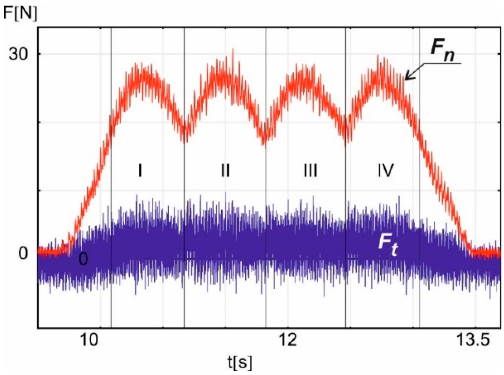
3. Experimental Results

In Figure 4, an example time plot of the tangential component Ft and the normal component Fn of the grinding force is presented, recorded during the working pass using the following machining parameters: ae = 0.01 mm and vw = 0.9 m/min.
As shown in the above graph, the shape of the course of both components of the grinding force depends on the length of contact between the grinding wheel and the workpiece. This length changes with the position of the grinding wheel relative to the gear-shaped sample with four teeth. For this reason, the graph is divided into four segments of force variability, corresponding to the four teeth of the hob cutter edge. These segments are numbered sequentially as I, II, III, and IV.
As can be observed in Figure 4, the highest value of the grinding normal force components in each of the four segments was obtained near the tooth tips, where the contact line is the longest. Similarly, the lowest value of the grinding force components was recorded at the tooth roots, where the contact line is the shortest.
It is worth noting that the presented force measurement is noisy. Fourier transformation showed that the noise frequency is close to the frequency associated with the variable dimensions of the gear-shaped sample.
The example time plot of the grinding force components shown in Figure 4 was obtained for one of the 54 measurements conducted under different machining conditions, considering three repetitions for each of the 18 sets of grinding parameters. To quantitatively compare the obtained results, the average value of Ft and Fn from segment II was calculated for each of the 54 working passes. This segment was taken from the full measurement, from the moment of reaching the minimum near segments I and II, to reaching the next minimum near segments II and III, as shown in Figure 4. Then, each of the three calculated average values for each of the 18 sets of grinding parameters was used to determine the average value of Ft and Fn representing a specific set of grinding parameters.
In Figure 5, the average normal component Fn of the grinding force is shown as a function of the workpiece speed vw and three different values of machining allowance ae. The smallest and largest values for each of the 18 sets of measurement results are also marked on the graph.
Similarly to the above, Figure 6 shows the average tangential component Ft of the grinding force as a function of the workpiece speed vw.
As shown in Figure 5 and Figure 6, increasing the workpiece speed vw at a constant grinding depth ae causes an increase in both the normal component Fn and the tangential component Ft of the grinding force. A similar effect is observed when increasing the grinding depth ae while maintaining a constant workpiece speed vw, as shown in Figure 7 and Figure 8. As expected, the smallest values of both Fn and Ft were achieved during grinding at the lowest workpiece speed (vw = 0.9 m/min), while simultaneously removing the smallest machining allowance (ae = 0.01 mm).

4. Force Models of Grinding Process

4.1. The Polynominal Model Force

The obtained experimental results allowed for the construction of a model for the normal component and the tangential component of the grinding force occurring during the hob cutter sharpening process. The models for the normal component Fn available in the literature gave divergent results compared to the conducted experiment. Ultimately, the best-fitting model was accepted, whose general form as a polynomial for the normal component Fn was presented by Werner in [18]:
F n = K · C 1 γ · Q w v s 2 1 · a e 1 · d s 1 ,
where K is the proportionality factor, C1 is the cutting edge density, γ is an exponent depending on the grinding parameter, Qw is the specific material removal rate, vs is the grinding wheel peripheral speed, is an exponent depending on the workpiece material, ae is a grinding depth, and ds is the diameter of the grinding wheel.
Based on Equation (1), our own mathematical model was proposed, encompassing both components of the grinding force, in the form of the equation:
F n , t v w , a e = K · v w v s 2 f 1 · a e D f · D ,
where
  • K—grinding coefficient, N/mm;
  • f—exponential coefficient;
  • vw—workpiece speed, m/min;
  • vs—grinding wheel peripheral speed, m/s;
  • ae—grinding depth, mm;
  • D—grinding wheel outer diameter, mm.
Based on the results obtained from the experimental studies, the parameters of the mathematical model were calculated using the least squares method, in the Mathematica software (version 8). After substituting them into Equation (2), two equations for calculating the components of the grinding force were obtained:
F n v w , a e = 506.751 · v w v s 0.3622 · a e D 0.6811 · D ,
F t v w , a e = 598.263 · v w v s 0.5995 · a e D 0.7998 · D ,
where
  • vs = 30.1 m/s;
  • D = 125 mm.
The multiple regression coefficient for these procedures was estimated at 0.9989 for normal force Fn and 0.9946 for tangential force Ft.

4.2. The Regression Analysis Procedure

To determine the mathematical relationships for calculating the normal component Fn and the tangential component Ft of the grinding force, the SKZ program (version 1.0) was used, which has been successfully developed and utilized by the authors in other research works [22,23,24]. The measured values from the experimental studies were used as input data.
The SKZ program determines the coefficients of the multiple regression equation using a regression analysis procedure based on the “acceptance and rejection” method [21]. The selection of critical values of the statistic (Fkr) is made at a significance level of α = 0.4, and after determining the regression function, it is changed to a value of α = 0.1. Calculations begin with the simplest regression function, sequentially adding new terms. When a newly added term reduces the significance of an already introduced term, it is considered insignificant and removed from the regression function. After introducing all significant terms, a panel with a preview of the calculation results is displayed on the monitor screen.
Ultimately, the function of the research object took the following general form:
F n , t = F 0 · v w f v · a e f a ,
where
  • F0—constant of the equation;
  • fv, fa—exponents of the equation.
The constants and coefficients determined from the calculations allowed for obtaining the relationship for the normal component Fn of the grinding force with a multiple correlation coefficient R = 0.8893:
F n = 876.6 · v w 0.338 · a e 0.685 .
Similar calculations allowed for obtaining the relationship for the tangential component Ft of the grinding force with a multiple correlation coefficient R = 0.8604:
F t = 775.9 · v w 0.529 · a e 1.052 .
The significance of the obtained multiple correlation coefficients R was determined using the Fisher–Snedecor F-test. For this purpose, the test values of the F factor were calculated and compared with the critical values Fkr. Since the F values are greater than the Fkr values, the correlation coefficients should be considered significant, which, as indicated in [25], entails the agreement (at a significance level of α = 0.1) of the regression function equation with the results of the conducted experimental studies.

4.3. Comparison of Models and Experiment Results

Despite the satisfactory values of the multiple correlation coefficients for the developed mathematical models, they were also verified by comparing the calculated values of the normal component Fn and the tangential component Ft of the grinding force with the values obtained during the experimental studies. For this purpose, the values of the grinding force components Fn and Ft were calculated for the 18 sets of grinding parameters used in the studies using Equations (6) and (7). Additionally, the values of both force components were also determined based on Equations (3) and (4) of the polynomial model.
In Figure 9, a comparison of the experimental results with the results obtained from the mathematical models describing the normal component Fn of the grinding force is presented. A similar graph showing the tangential component Ft of the grinding force is shown in Figure 10.
The calculation results of Fn and Ft obtained from the two presented models are summarized in Table 2 and Table 3, respectively. In the case of the normal component Fn of the grinding force, the relative errors of the models are larger compared to those obtained for the tangential component Ft of the grinding force. The largest relative error for Fn in the regression model occurs at a grinding depth ae = 0.01 mm (( ¯ ) = 3.820%), while for the polynomial model it occurs at a grinding depth ae = 0.02 mm (( ¯ ) = 3.922%). Nevertheless, the overall average errors for both models remain relatively small, amounting to 3.241% for the regression model and 3.228% for the polynomial model.
It is worth noting that the largest relative error for the models of the tangential component Ft of the grinding force is observed in the regression model (( ¯ ) = 2.016%) and the polynomial model (( ¯ ) = 2.755%) at the same grinding depth ae = 0.01 mm, which is the smallest. The overall average error for both models is quite small, amounting to 1.409% for the regression model and 1.727% for the polynomial model.
Analyzing Table 2 and Table 3, as well as Figure 9 and Figure 10, it can be seen that both models effectively replicate the experimental results. In the case of the normal component Fn, the results obtained from both models are almost identical, while for the tangential component Ft, the results show a very small relative error despite the irregular course of the experimental results. Therefore, the results calculated based on the presented models and the results obtained from the experiment are consistent with each other.

5. Conclusions

The article presents mathematical models in the form of multiple regression functions and polynomial functions, enabling the calculation of the normal component Fn and the tangential component Ft of the grinding force during the sharpening of the rake surfaces of hob cutters. The models were determined based on the results of experimental studies.
Based on the obtained research results, it can be concluded that:
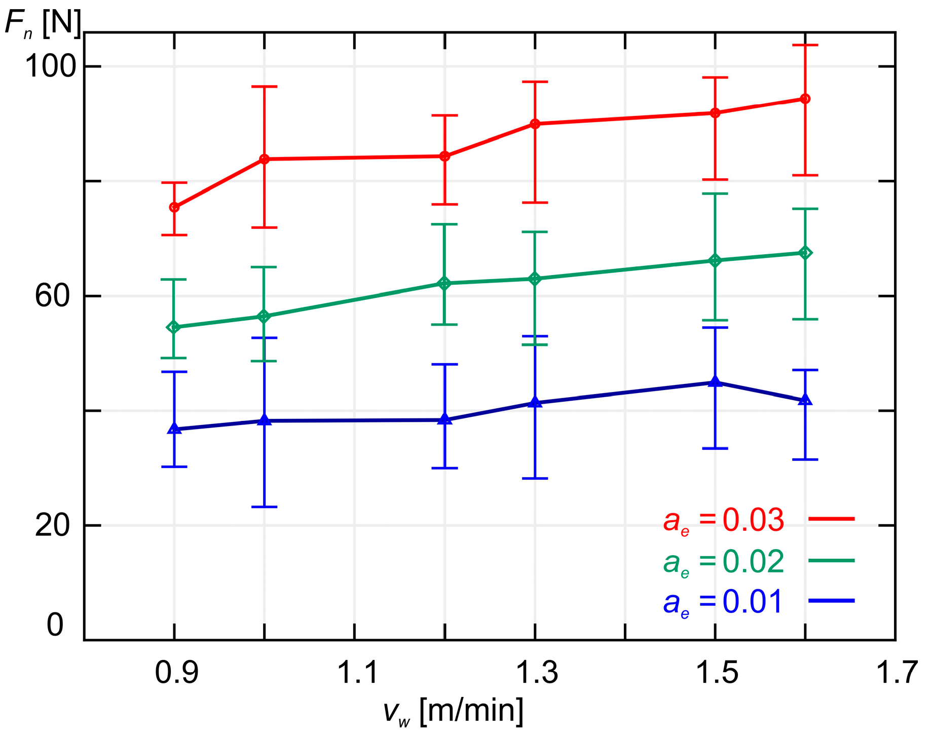
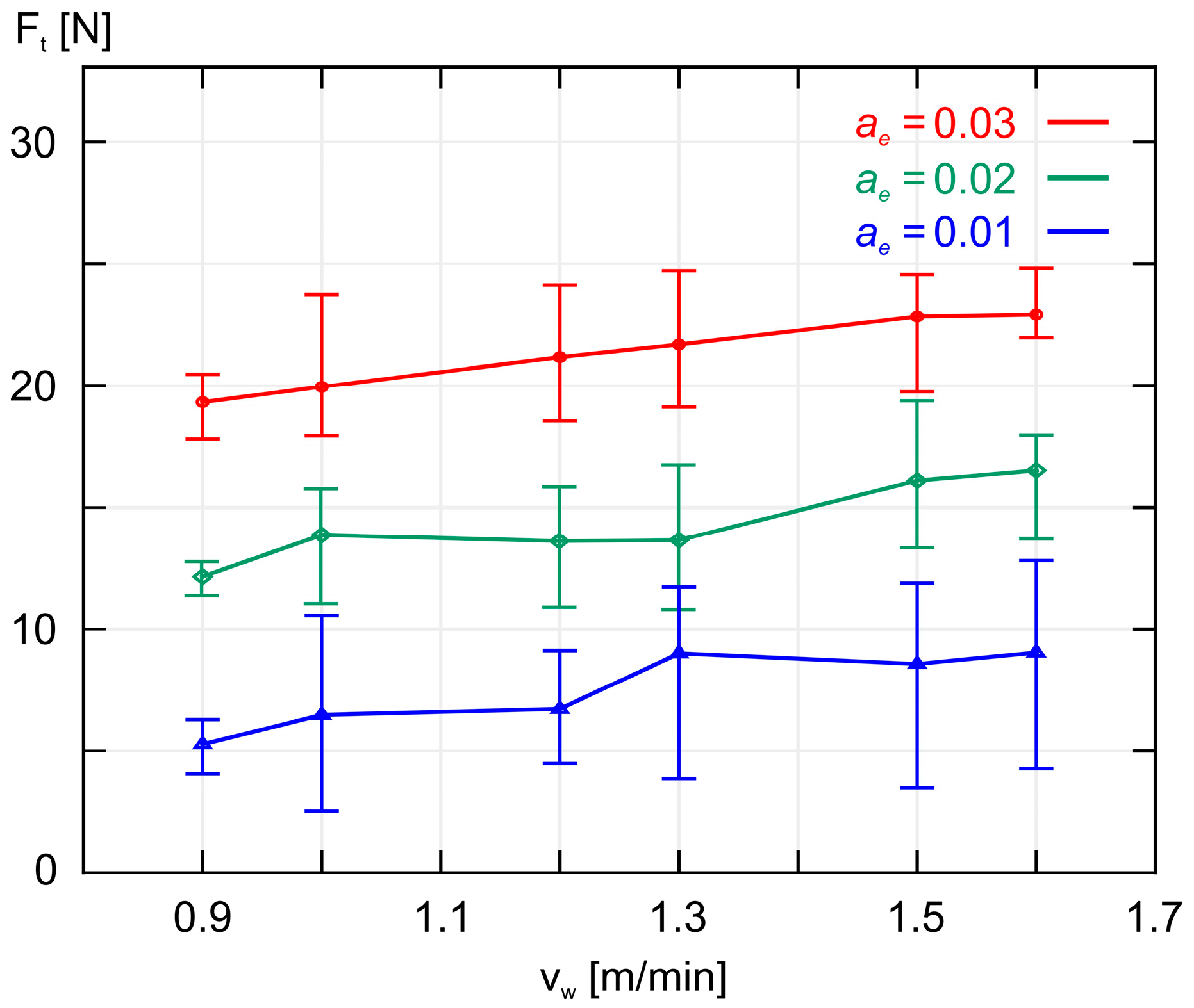
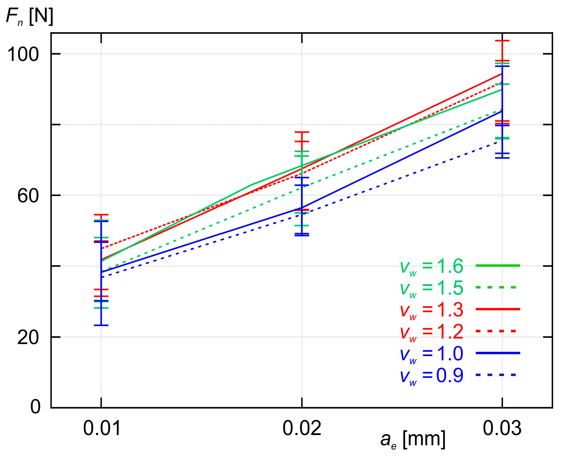
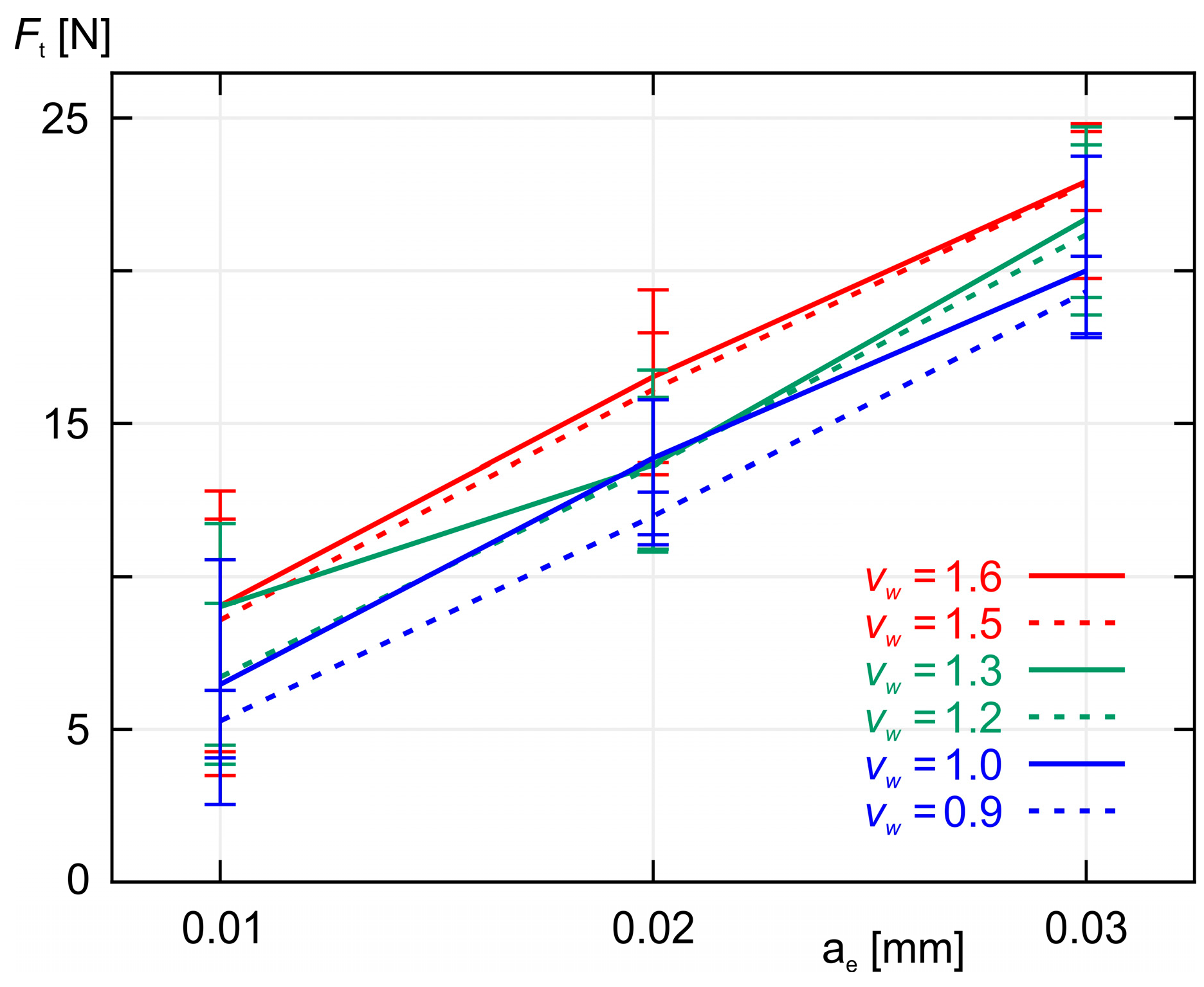
  • Both the experimental results and the results obtained from the calculations based on the models indicate that as the grinding depth ae increases, the values of the grinding force components (Fn and Ft) also increase, which was expected. A similar relationship was found when the workpiece speed vw was increased.
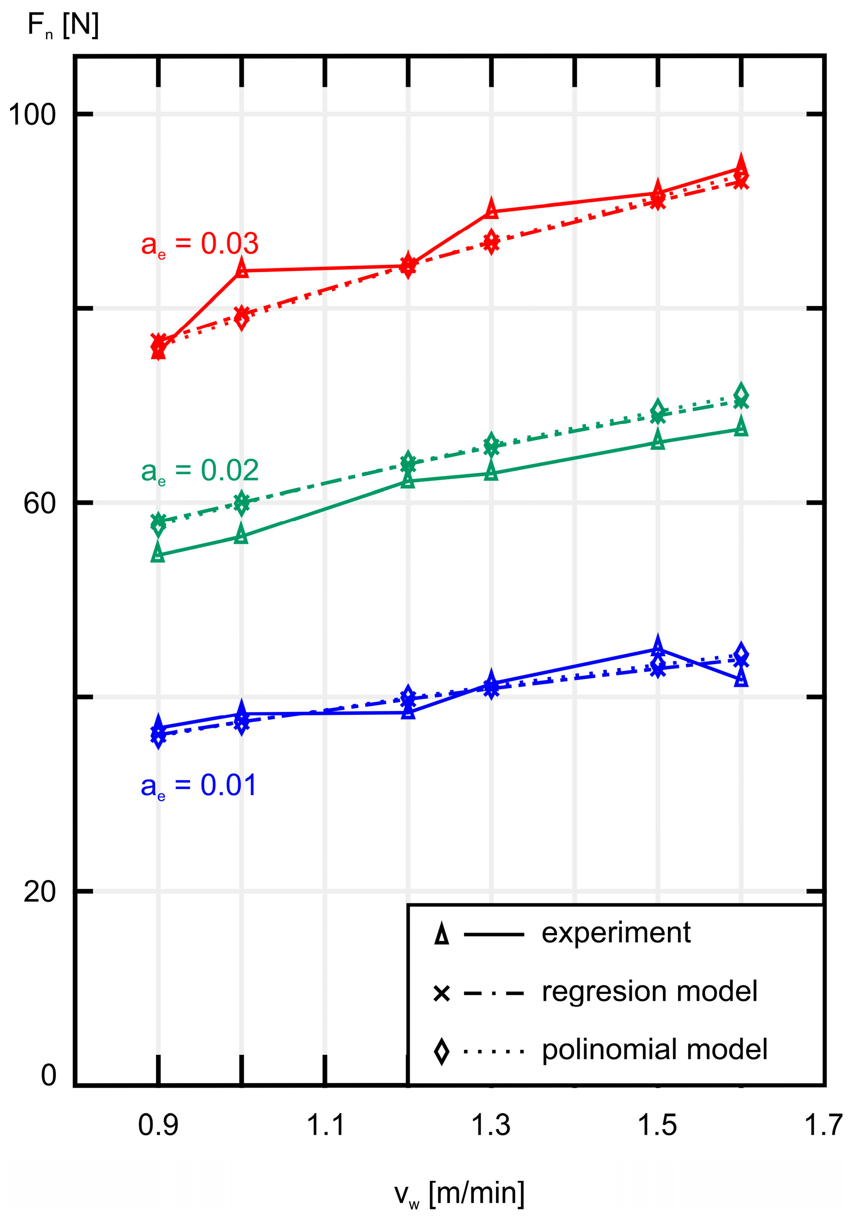
  • In the case of the normal component Fn, the overall percentage average errors for both models remain small, amounting to 3.241% for the regression model and 3.228% for the polynomial model. For the tangential component Ft, the overall percentage average error for both models is small, amounting to 1.409% for the regression model and 1.727% for the polynomial model.
  • The values of both grinding force components calculated based on the mathematical models are consistent with the results obtained from the experiment. In the case of the Fn component, the calculated values in both cases deviate insignificantly from the experimental values, while for the Ft component, the results show a very small relative error despite the irregular course of the experimental results, which should be considered very satisfactory. Additionally, the high value of the multiple regression coefficient for both models demonstrates compliance with the experimental results.
  • The developed models provide a good basis for analyzing the hob cutter sharpening process with variable grinding parameters, and can also be used in modelling the dynamic grinding process.

Author Contributions

Conceptualization, B.W., W.S. and M.S.; Methodology, B.W., W.S. and M.S.; Software, B.W. and W.S.; Validation, B.W., W.S. and N.K.; Formal analysis, B.W., W.S. and W.P.; Investigation, B.W. and W.S.; Data curation, B.W. and W.S.; Writing—original draft, B.W. and W.S.; Writing—review and editing, B.W., W.S., N.K. and W.P. All authors have read and agreed to the published version of the manuscript.

Funding

This research received no external funding.

Institutional Review Board Statement

Not applicable.

Informed Consent Statement

Not applicable.

Data Availability Statement

Data are contained within the article.

Conflicts of Interest

The authors declare no conflicts of interest.

References

  1. Korecki, M.; Wołowiec-Korecka, E. Glenn. Single-piece, high-volume, low-distortion case hardening of gears. Therm. Process. 2016, 9, 32–39. [Google Scholar]
  2. Stachurski, W.; Sawicki, J.; Wójcik, R.; Nadolny, K. Influence of application of hybrid MQL-CCA method of applying coolant during hob cutter sharpening on cutting blade surface condition. J. Clean. Prod. 2018, 171, 892–910. [Google Scholar] [CrossRef]
  3. Moderow, R. The right and wrong of modern hob sharpening. Gear Technol. 1992, 34–38. [Google Scholar]
  4. Kruszyński, B.; Wójcik, R. Residual stress in grinding. J. Mater. Process. Technol. 2001, 109, 254–257. [Google Scholar] [CrossRef]
  5. Malkin, S.; Guo, C. Grinding Technology: Theory and Applications of Machining with Abrasives, 2nd ed.; Industrial Press Inc.: New York, NY, USA, 2008. [Google Scholar]
  6. Stachurski, W.; Nadolny, K. Influence of the condition of the surface layer of a hob cutter sharpened using the MQL-CCA hybrid method of coolant provision on its operational wear. Int. J. Adv. Manuf. Technol. 2018, 98, 2185–2200. [Google Scholar] [CrossRef]
  7. Rowe, W.B. Principles of Modern Grinding Technology, 2nd ed.; Elsevier: Amsterdam, The Netherlands, 2014. [Google Scholar]
  8. Stachurski, W.; Dębkowski, R.; Rosik, R.; Święcik, R.; Pawłowski, W. Evaluation of the influence of the cooling method used during grinding on the operating properties of ceramic grinding wheels made with different abrasives. Adv. Sci. Technol. Res. J. 2023, 17, 1–18. [Google Scholar] [CrossRef]
  9. Li, L.; Zhang, Y.; Cui, X.; Said, Z.; Sharma, S.; Liu, M.; Gao, T.; Zhou, Z.; Wang, X.; Li, C. Mechanical behavior and modeling of grinding force: A comparative analysis. J. Manuf. Process. 2023, 102, 921–954. [Google Scholar] [CrossRef]
  10. Li, B.; Li, X.; Hou, S.; Yang, S.; Li, Z.; Qian, J.; He, Z. Prediction and analysis of grinding force on grinding heads based on grain measurement statistics and single-grain grinding simulation. Int. J. Adv. Manuf. Technol. 2024, 132, 513–532. [Google Scholar] [CrossRef]
  11. Wang, X.; Liu, Q.Y.; Zheng, Y.; Xing, W.; Wang, M. A grinding force prediction model with random distribution of abrasive grains: Considering material removal and undeformed chips. Int. J. Adv. Manuf. Technol. 2022, 120, 7219–7233. [Google Scholar] [CrossRef]
  12. Wu, Z.; Zhang, L. Analytical grinding force prediction with random abrasive grains of grinding wheels. Int. J. Mech. Sci. 2023, 250, 108310. [Google Scholar] [CrossRef]
  13. Yan, Y.; Xu, J.; Wiercigroch, M. Non-linear analysis and quench control of chatter in a plunge grinding. Int. J. Non-Linear Mech. 2015, 70, 134–144. [Google Scholar] [CrossRef]
  14. Yan, Y.; Xu, J.; Wiercigroch, M. Regenerative chatter in self-interrupted plunge grinding. Meccanica 2016, 51, 3185–3202. [Google Scholar] [CrossRef]
  15. Yan, Y.; Xu, J.; Wiercigroch, M. Regenerative chatter in a plunge grinding process with workpiece imbalance. Int. J. Adv. Manuf. Technol. 2017, 89, 2845–2862. [Google Scholar] [CrossRef]
  16. Yan, Y.; Xu, J.; Wiercigroch, M. Chatter in a transverse grinding process. J. Sound Vib. 2014, 333, 937–953. [Google Scholar] [CrossRef]
  17. Sun, C.; Deng, Y.; Lan, D.; Xiu, S. Modeling and predicting ground surface topography on grinding chatter. Procedia CIRP 2018, 71, 364–369. [Google Scholar] [CrossRef]
  18. Werner, G. Influence of work material on grinding forces. Ann. CIRP 1978, 27, 243–248. [Google Scholar]
  19. Meng, Q.; Guo, B.; Zhao, Q.; Li, H.N.; Jackson, M.J.; Linke, B.S.; Luo, X. Modelling of grinding mechanics: A review. Chin. J. Aeronaut. 2022, 36, 25–39. [Google Scholar] [CrossRef]
  20. Mishra, V.K.; Salonitis, K. Empirical estimation of grinding specific forces and energy based on a modified Werner grinding model. Procedia CIRP 2013, 8, 287–292. [Google Scholar] [CrossRef]
  21. Cieciura, M.; Zacharski, J. Probabilistic Methods in Practice; Vizja Press & IT: Warsaw, Poland, 2007. [Google Scholar]
  22. Kruszyński, B.; Midera, S.; Kaczmarek, J. Forces in generating gear grinding-theoretical and experimental approach. CIRP Ann.–Manuf. Technol. 1998, 47, 287–290. [Google Scholar] [CrossRef]
  23. Stachurski, W.; Midera, S.; Kruszyński, B. Mathematical model describing the course of the process of wear of a hob cutter for various methods of cutting fluid supply. Eksploat. Niezawodn. 2016, 18, 123–127. [Google Scholar] [CrossRef]
  24. Stachurski, W.; Sawicki, J.; Krupanek, K.; Midera, S. Mathematical model for determining the expenditure of cooling and lubricating fluid reaching directly the grinding zone. Arch. Mater. Sci. Eng. 2018, 94, 27–34. [Google Scholar] [CrossRef]
  25. Korzyński, M. Methodology of the Experiment-Planning, Implementation and Statistical Analysis of the Results of Technological Experiments; WNT: Warsaw, Poland, 2013. [Google Scholar]
Figure 1. A general view of the ASP-631 F-SL tool grinder (Lakfam, Kowary, Poland).
Materials 18 00138 g001
Figure 2. A view of the workspace of the ASP-631 F-SL tool grinder.
Materials 18 00138 g002
Figure 3. Distribution of grinding force components: Ft—tangential component; Fn—normal component; ns—grinding wheel rotational speed; vw—workpiece speed.
Materials 18 00138 g003
Figure 4. A sample time course of the tangential component Ft and the normal component Fn of the grinding force during the working pass; ae = 0.01 mm, vw = 0.9 m/min, sampling frequency 10 kHz.
Materials 18 00138 g004
Figure 5. A plot of the average values of the normal component Fn of the grinding force as a function of the workpiece speed vw for three different values of machining allowance ae.
Materials 18 00138 g005
Figure 6. A plot of the average values of the tangential component Ft of the grinding force as a function of the workpiece speed vw for three different values of machining allowance ae.
Materials 18 00138 g006
Figure 7. A plot of the average values of the normal component Fn of the grinding force as a function of the machining allowance ae for six different values of workpiece speed vw.
Materials 18 00138 g007
Figure 8. A plot of the average values of the tangential component Ft of the grinding force as a function of the machining allowance ae for six different values of workpiece speed vw.
Materials 18 00138 g008
Figure 9. A plot of the experimental (solid line), regression model (point line), and polynomial model (dotted line) values of mean normal forces Fn versus workpiece speed vw for three grinding depths ae.
Materials 18 00138 g009
Figure 10. A plot of the experimental (solid line), regression model (point line), and polynomial model (dotted line) values of mean tangential forces Ft versus workpiece speed vw for three grinding depths ae.
Materials 18 00138 g010
Table 1. Grinding conditions used during experimental tests.
Workpiece materialHS6-5-2, carburized and hardened with 62 ± 1 HRC
Grinding wheel38A60KVBE
Grinding wheel rotational speedns = 4600 rpm
Grinding wheel peripheral speedvs = 30.1 m/s
Workpiece speedvw1 = 0.9 m/min
vw2 = 1.0 m/min
vw3 = 1.2 m/min
vw4 = 1.3 m/min
vw5 = 1.5 m/min
vw6 = 1.6 m/min
Machining allowance (working engagement, grinding depth)ae1 = 0.01 mm
ae2 = 0.02 mm
ae3 = 0.03 mm
Number of passes: grinding/return1/1
Grinding directionUp grinding
DresserSingle-point diamond dresser
Dresser weightQd = 1.0 kt (0.2 g)
Grinding wheel peripheral speed while dressingvsd = 30.1 m/s
Dressing allowancead = 0.01 mm
Axial table feed speed while dressingvfd = 40 mm/min
Number of dressing passesid = 10
EnvironmentsWET—conventional flood method
CoolantAGIP Aquamet 104 Plus in a 5% concentration
Coolant flow rateQ = 3 L/min
Table 2. The values of the normal component Fn of the grinding force obtained experimentally and calculated based on models.
Input DataRegression ModelPolynomial Model
vw [m/min]ae [mm]Normal Force Fn [N]
(Experiment)
Normal Force Fn [N]
(Regression Model)
Error
|Δ|
Percentage Error
| Δ | F t · 100%
Average Error
| Δ i | n
Percentage Average Error
| Δ i | F t n 100 %
Normal Force Fn [N]
(Polynomial Model)
Error
|Δ|
Percentage Error
| Δ | F t · 100%
Average Error
| Δ i | n
Percentage Average Error
| Δ i | F t n 100 %
0.90.0137.79936.0861.7134.5331.5973.82035.9681.8314.8441.6203.896
1.039.29437.3941.9004.83537.3671.9274.903
1.239.43839.7710.3330.84439.9180.4801.218
1.342.40540.8621.5433.64041.0921.3133.095
1.545.96642.8863.0806.70043.2782.6885.847
1.642.81743.8321.0152.37144.3021.4853.468
0.90.0255.13558.0152.8805.2242.3063.77057.6702.5354.5982.4243.922
1.057.04460.1183.0745.38959.9132.8695.030
1.262.76463.9401.1761.87364.0031.2391.975
1.363.55765.6932.1363.36165.8862.3293.664
1.566.74568.9492.2043.30269.3912.6463.964
1.668.10570.4692.3643.47171.0322.9274.298
0.90.0375.48076.5881.1081.4691.8412.13276.0130.5330.7061.6111.868
1.083.82879.3654.4635.32478.9694.8595.796
1.284.34084.4100.0700.08384.3600.0200.024
1.389.93286.7253.2073.56686.8423.0903.436
1.591.84291.0220.8200.89291.4620.3800.414
1.694.40893.0301.3781.46093.6250.7830.830
Total average error:1.9153.241Total average error:1.8853.228
Table 3. The values of the tangential component Ft of the grinding force obtained experimentally and calculated based on models.
Input DataRegression ModelPolynomial Model
vw [m/min]ae [mm]Tangential Force Ft [N]
(Experiment)
Tangential Force Ft [N]
(Regression Model)
Error
|Δ|
Percentage Error
| Δ | F t · 100%
Average Error
| Δ i | n
Percentage Average Error
| Δ i | F t n 100 %
Tangential Force Ft [N]
(Polynomial Model)
Error
|Δ|
Percentage Error
| Δ | F t · 100%
Average Error
| Δ i | n
Percentage Average Error
| Δ i | F t n 100 %
0.90.015.2805.7760.4961.3110.8552.0167.0691.7894.7321.1122.755
1.06.4766.1070.3690.9407.5291.0532.681
1.26.7196.7250.0060.0158.3991.6804.260
1.39.0267.0162.0104.7408.8120.2140.505
1.58.5877.5681.0192.2189.6011.0142.207
1.69.0607.8301.2302.8729.9800.9202.149
0.90.0212.50111.9750.5260.9540.7241.18512.3050.1960.3560.6281.025
1.014.27212.6621.6102.82313.1071.1652.042
1.214.01313.9440.0690.11114.6210.6080.969
1.314.05314.5470.4940.77715.3401.2872.025
1.516.57215.6910.8811.32016.7140.1420.213
1.617.00116.2360.7651.12417.3730.3720.547
0.90.0319.33818.3460.9921.3150.9011.02517.0182.3203.0741.1631.402
1.019.97519.3970.5780.68918.1281.8472.204
1.221.19721.3610.1640.19520.2210.9761.157
1.321.71622.2850.5690.63321.2150.5010.557
1.522.86524.0381.1731.27723.1160.2510.273
1.622.94524.8721.9272.04224.0281.0831.147
Total average error:0.8271.409Total average error:0.9681.727
Disclaimer/Publisher’s Note: The statements, opinions and data contained in all publications are solely those of the individual author(s) and contributor(s) and not of MDPI and/or the editor(s). MDPI and/or the editor(s) disclaim responsibility for any injury to people or property resulting from any ideas, methods, instructions or products referred to in the content.

