
Numerical Simulation of Moisture Diffusion in the Microstructure of Asphalt Mixtures

Abstract
:1. Introduction
- (1)
- A model that regards an asphalt mixture as a homogeneous material [18]. As such, the amount of data is small and the model operation simple. Because an asphalt mixture is a kind of porous material, there are a large number of pores in the mixture, and these pores comprise the main path of water vapour diffusion. Therefore, ignoring the internal structure of an asphalt mixture will cause a simulation result to deviate from the actual situation.
- (2)
- A model that regards an asphalt mixture as a combination of a fine aggregate–asphalt mixture (aggregate size ≤ 1.18 mm + pore + asphalt) and coarse aggregate (aggregate size > 1.18 mm) [14,19]. In this type of finite element model, the diffusivities of a fine aggregate–asphalt mixture are equal to the effective diffusivities of an asphalt mixture. As a fine aggregate–asphalt mixture and an asphalt mixture have completely different framework structures, they are unlikely to have the same diffusivity as water vapour [1]. Therefore, using this type of model will lead to a great difference between the numerical results and the experimental results.
2. Geometric Model of the Microstructure of the Asphalt Mixture
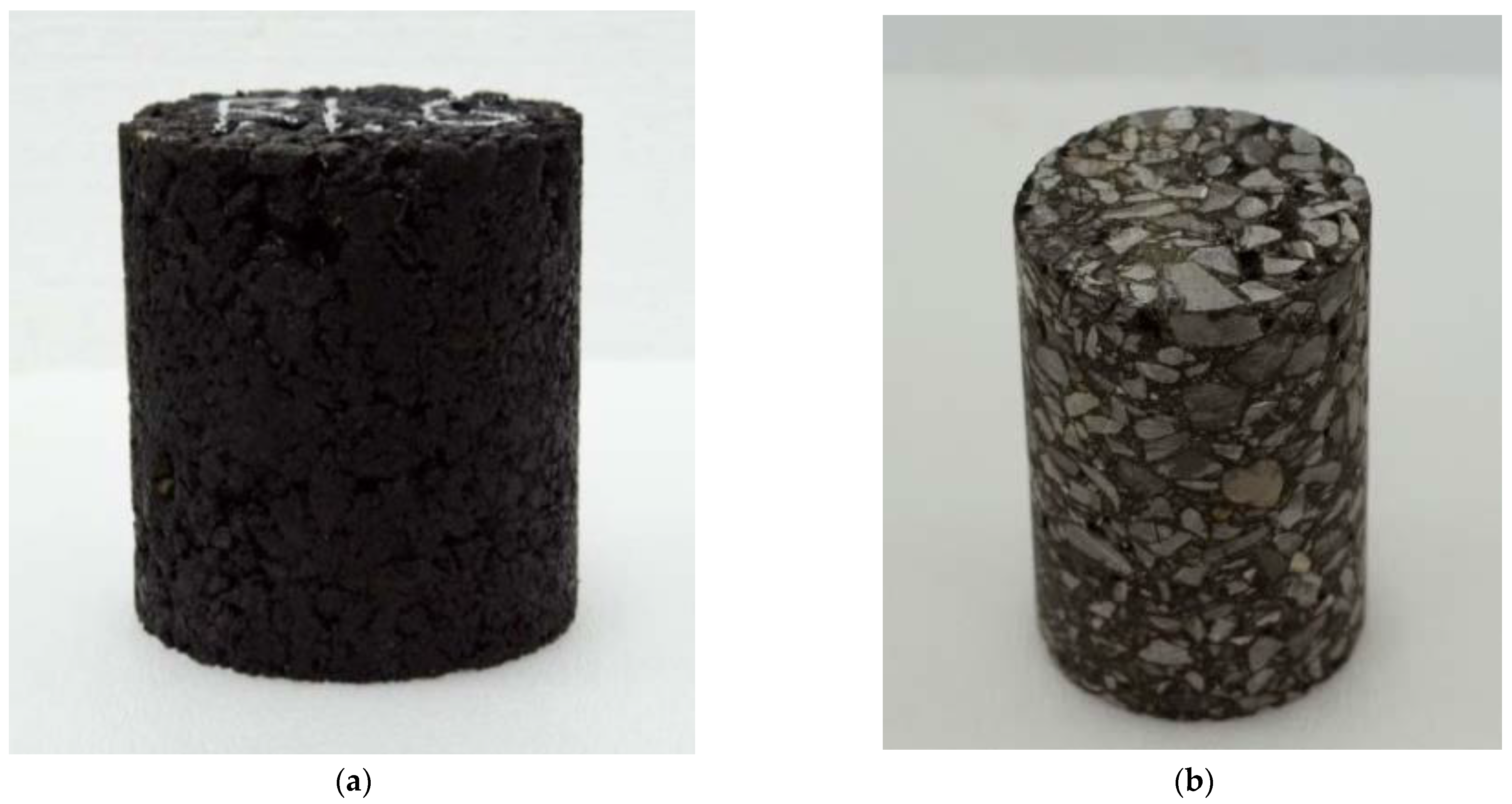
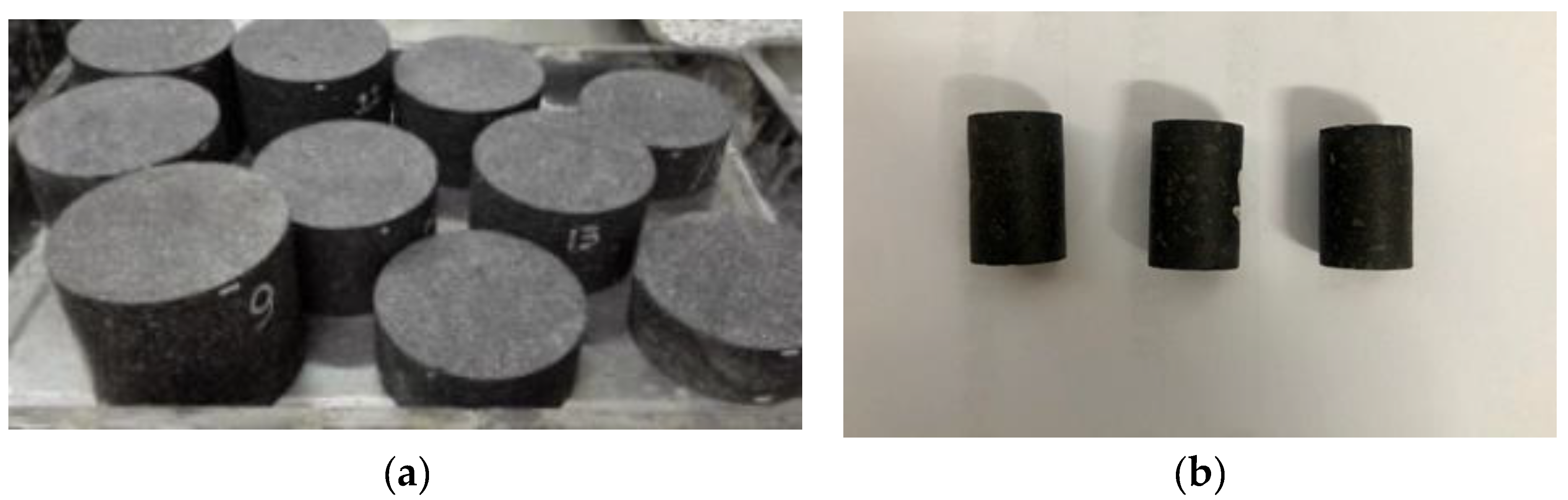
2.1. Preparation of the Asphalt Mixture Specimen
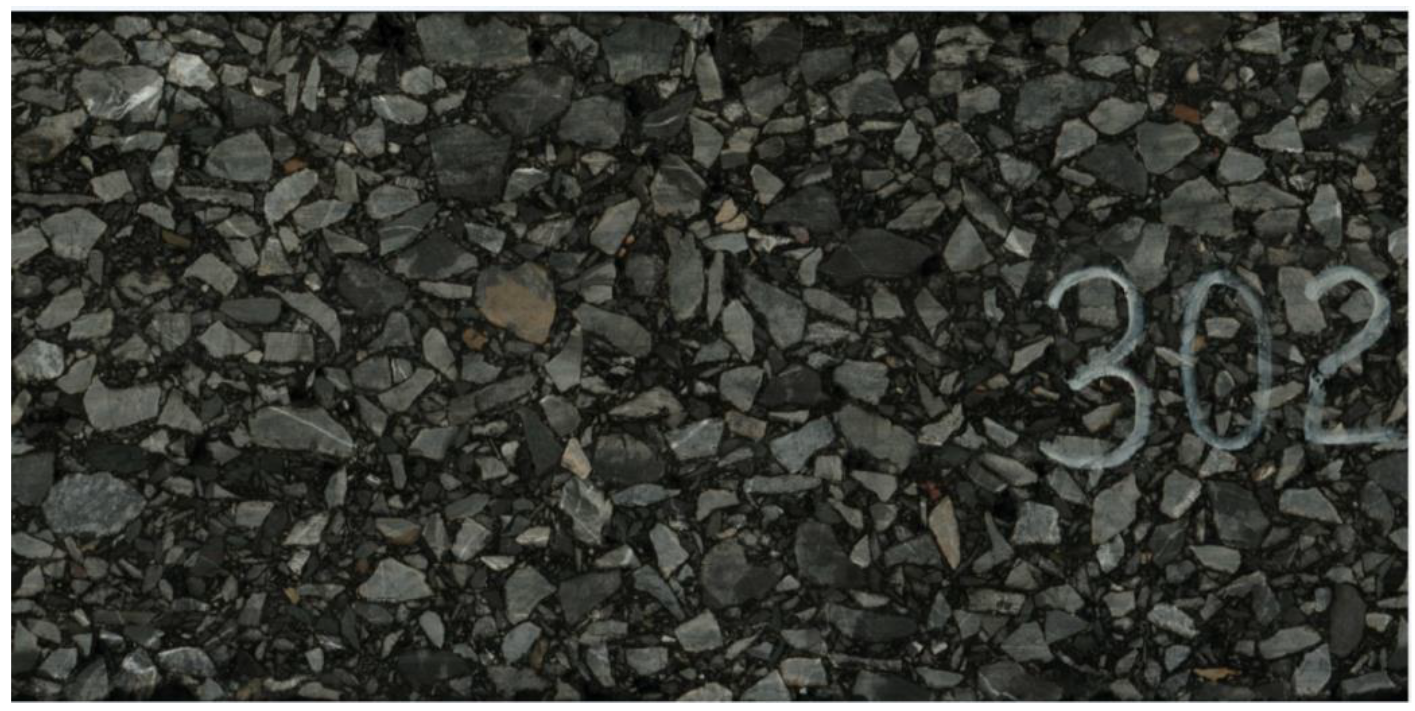
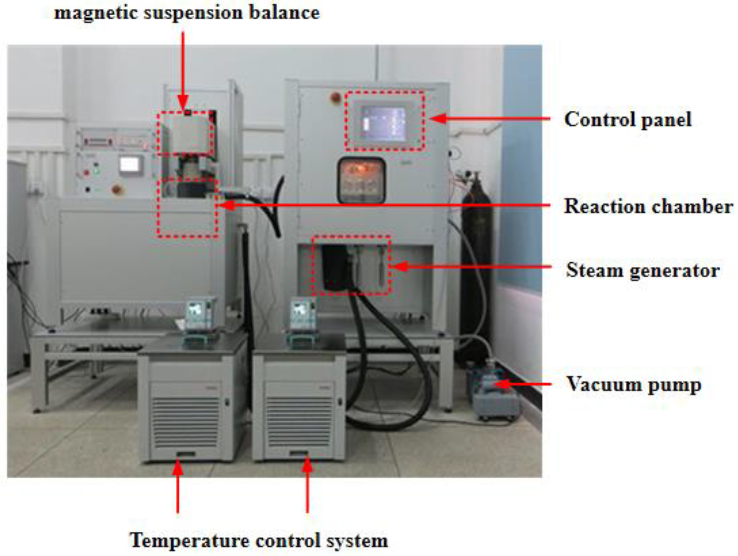
2.2. Scanning the Asphalt Mixture Specimen
2.3. Establishing the Geometric Asphalt Mixture Model
- (1)
- (2)
- Voids could not be distinguished from asphalt within the images [24].
3. Water Vapour Diffusivities of the Asphalt Mixture in the Numerical Model
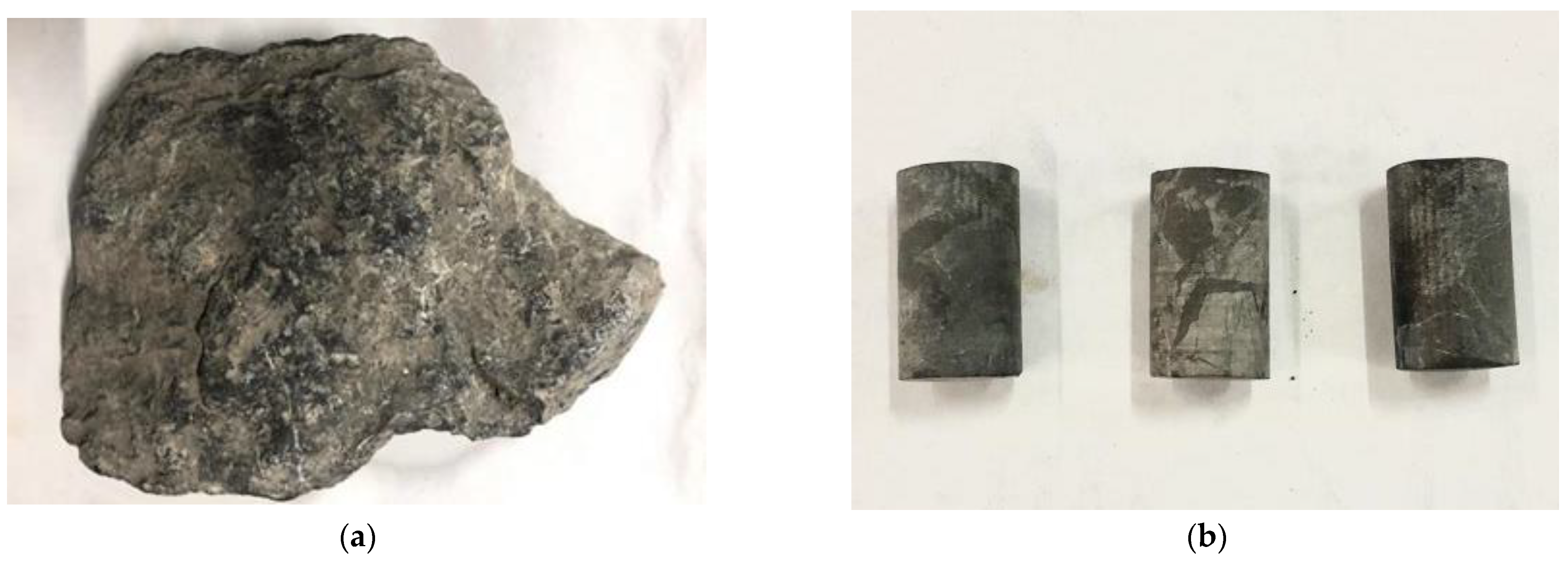
3.1. Water Vapour Diffusivities of Medium I
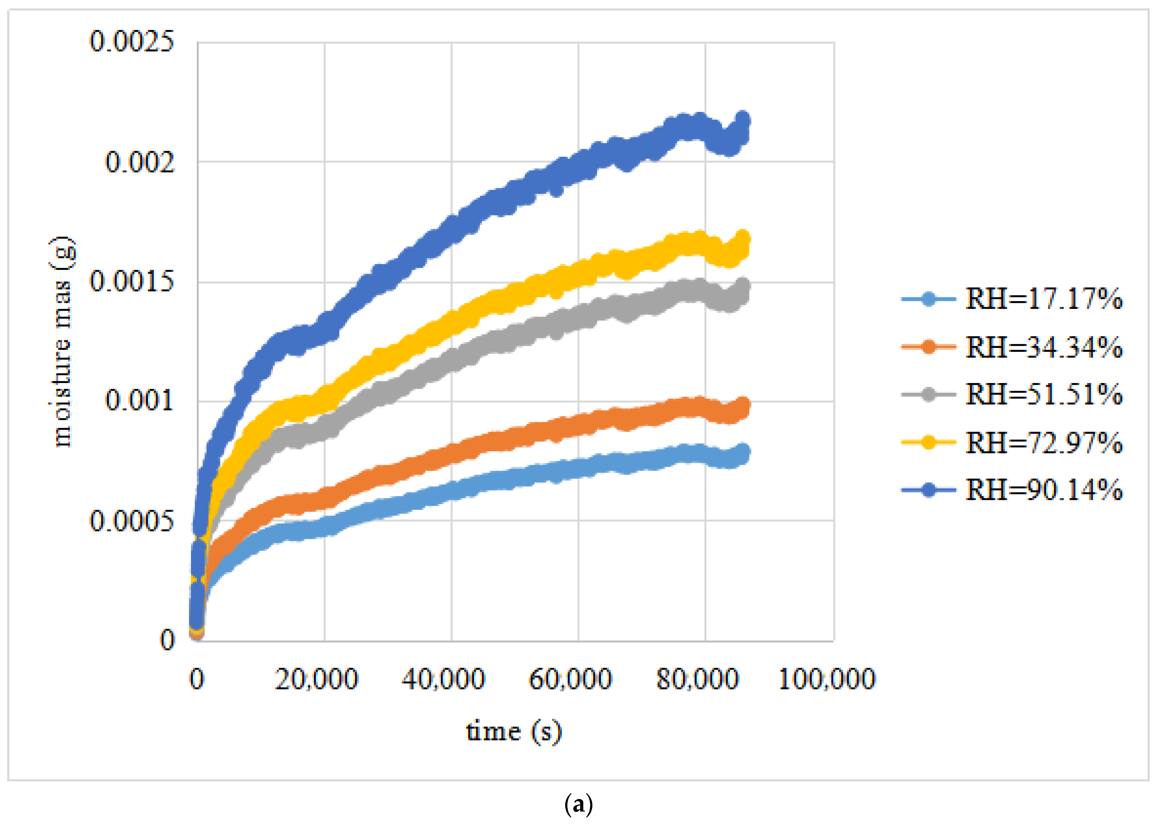
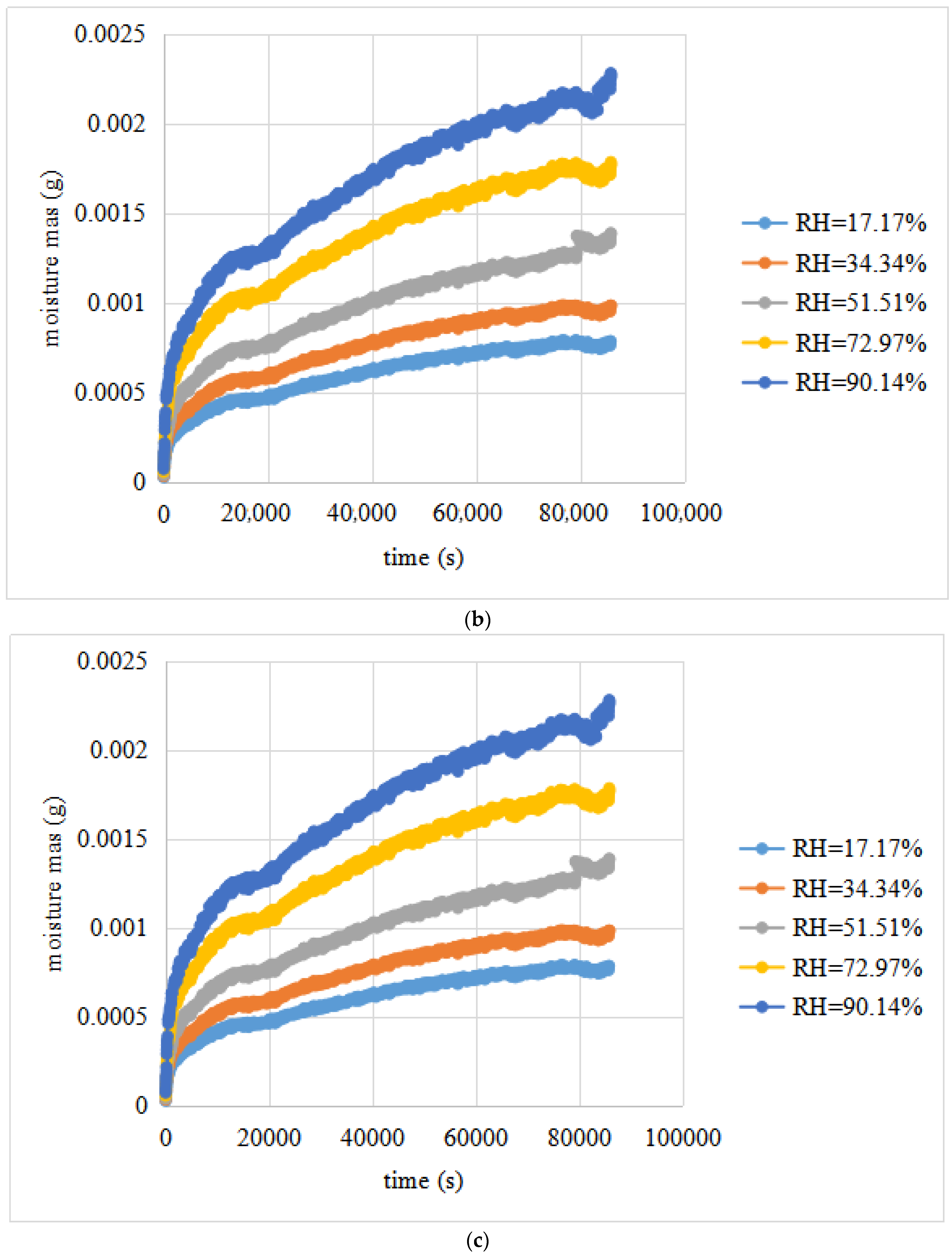
- (a).
- The parameter M(t) exhibited an excellent relationship with t, and every fitting model had an R2 value larger than 0.90.
- (b).
- The fitting curves of the test data of the replicated setups for the same RH differential were fairly close to each other, which demonstrated the repeatability of the designed water vapour diffusion tests.
- (c).
- The average water vapour diffusivities of the limestone were 6.7299 × 10⁻⁴ mm2/s. For different relative humidity conditions, the water vapour diffusivities of the same limestone sample showed little difference, and the CV was less than 10%. This shows that the water vapour diffusivities of the limestone change little with relative humidity.
3.2. Water Vapour Diffusivities of Medium II
3.3. Water Vapour Diffusivities of Medium III
3.3.1. Void Characteristics of the Fine Aggregate–Asphalt Mixture
3.3.2. Calculation of the Diffusivities of Medium III
- (1)
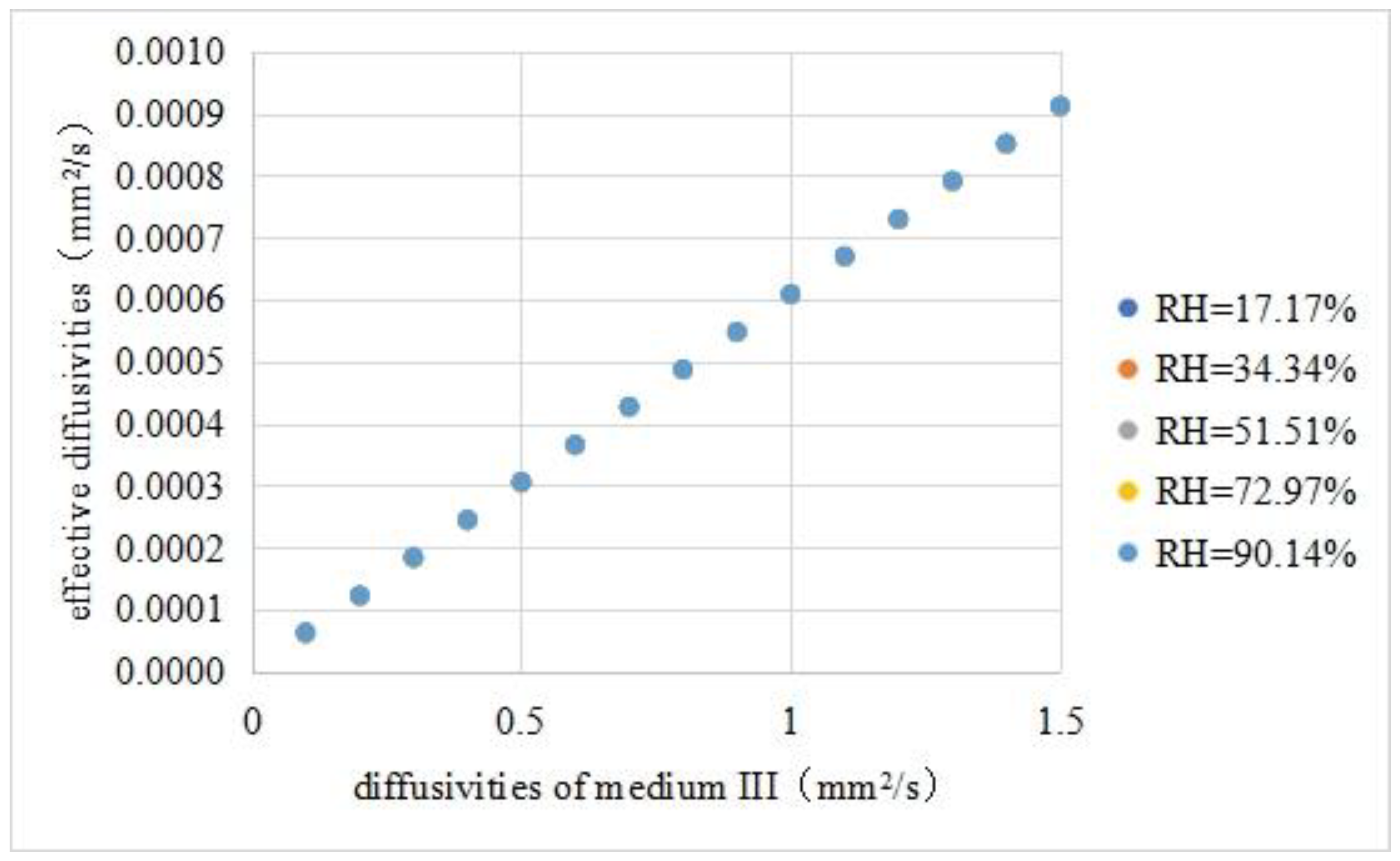
- Effective diffusivities vs. diffusivities of medium III
- 1.
- The effective diffusivities and medium III diffusivities were fitted with a linear equation. The fitting results are shown in Equation (18). The fitness was 0.9999.
- 2.
- The effective diffusivities of the asphalt mixture did not change significantly with the external relative humidity, indicating that the effective diffusivities were mainly affected by the diffusivities of each component and the internal structure.
- 3.
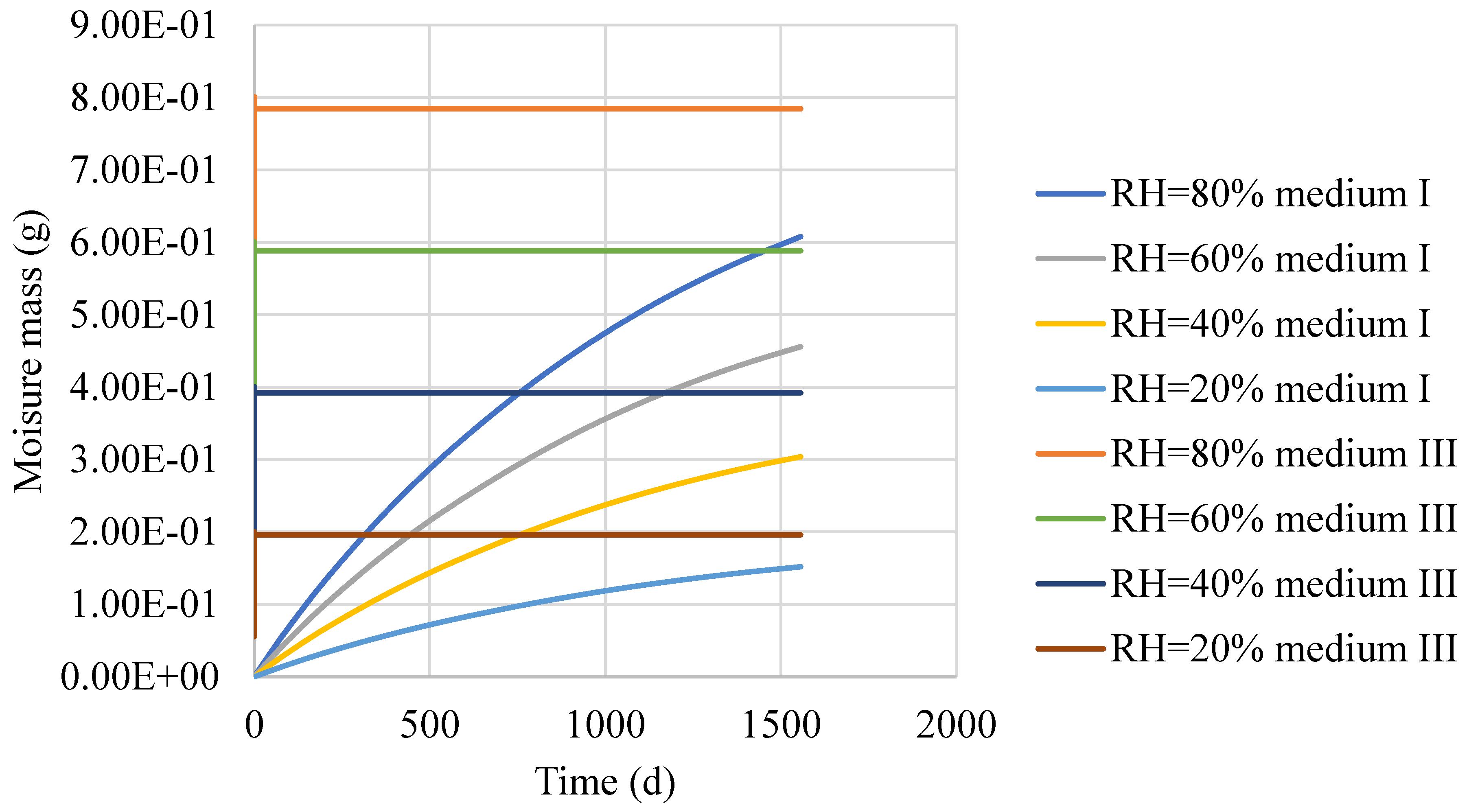
- The effective diffusivities of the asphalt mixture had an order of magnitude of 10−4 mm2/s, and the diffusivities of medium III in the asphalt mixture had an order of magnitude of mm2/s, with a difference of 104. Therefore, the effective diffusivities were used to directly simulate the moisture diffusion of the asphalt mixture, resulting in serious underestimation of the moisture movement rate.
- (2)
- Diffusivities of medium III in the asphalt mixture
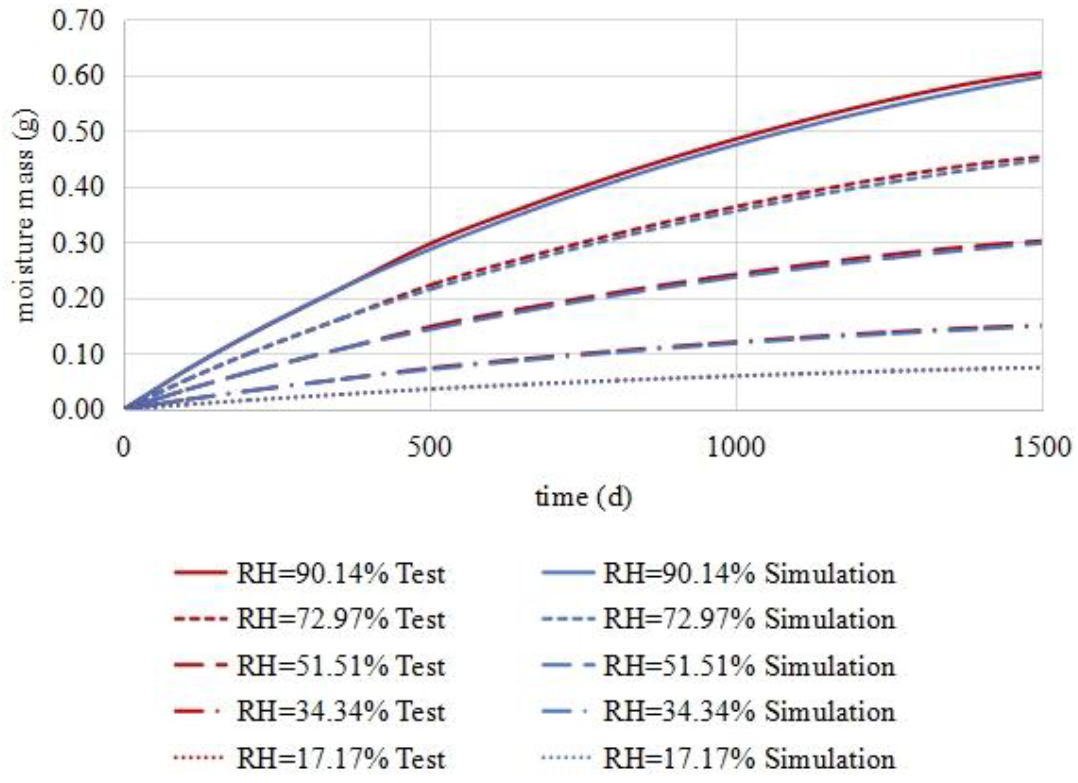
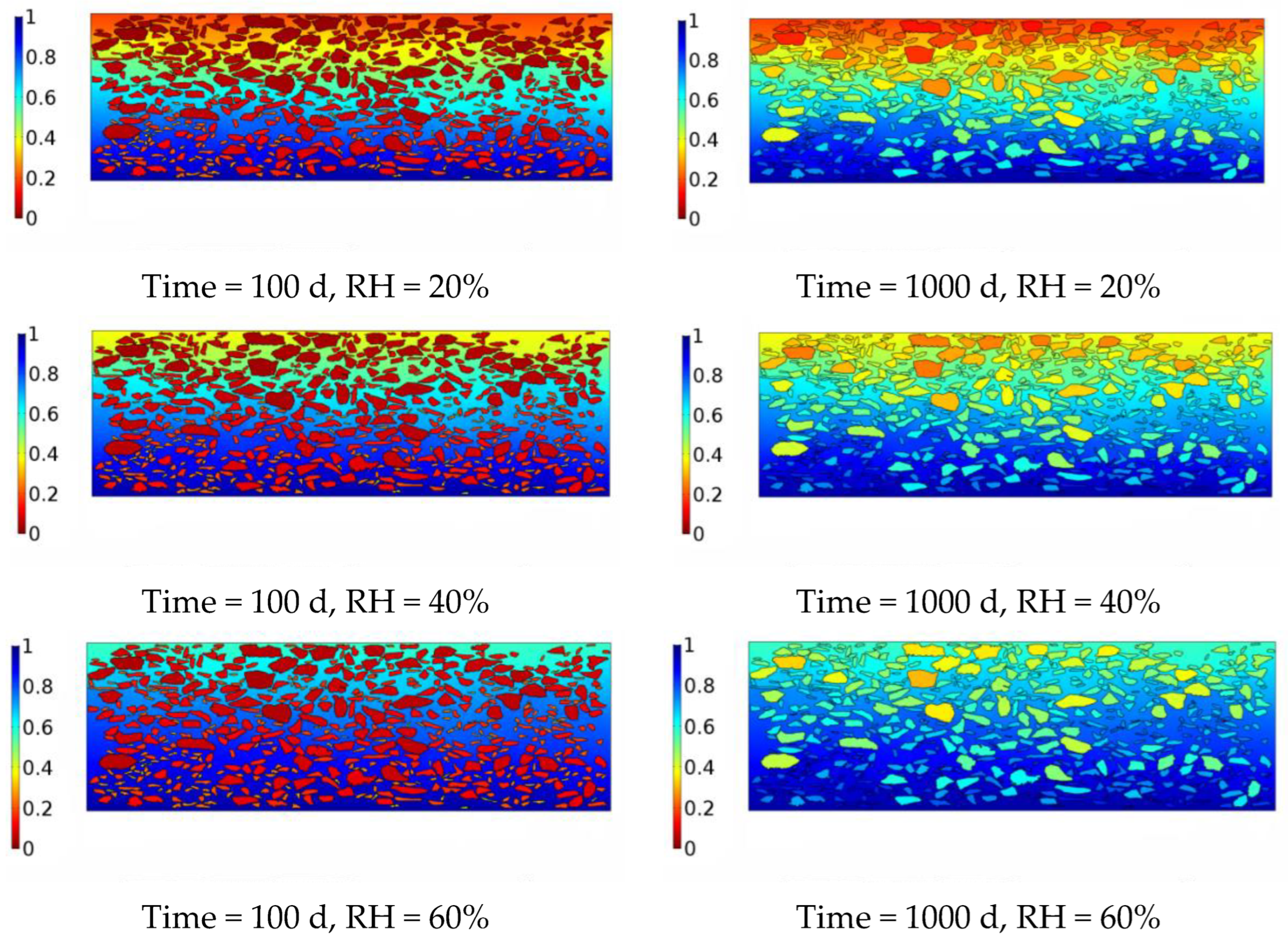
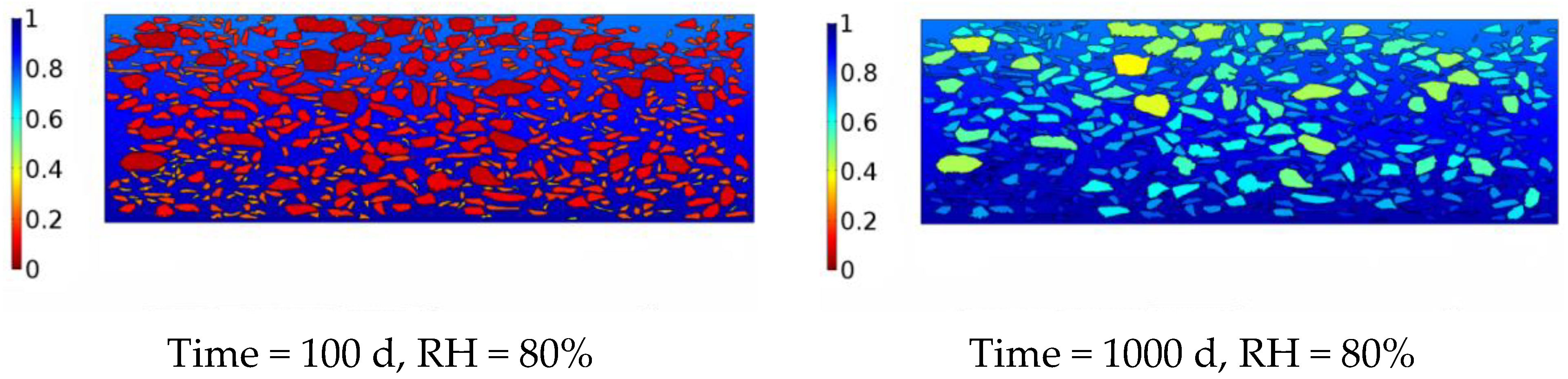
4. Numerical Model of Moisture Diffusion in the Asphalt Mixture
5. Conclusions
Author Contributions
Funding
Institutional Review Board Statement
Informed Consent Statement
Data Availability Statement
Acknowledgments
Conflicts of Interest
References
- Luo, R.; Tu, C. Actual diffusivities and diffusion paths of water vapor in asphalt mixtures. Constr. Build. Mater. 2019, 207, 145–157. [Google Scholar] [CrossRef]
- Vasconcelos, K.L.; Bhasin, A.; Little, D.N. Measurement of Water Diffusion in Asphalt Binders Using Fourier Transform Infrared-Attenuated Total Reflectance. Transp. Res. Rec. 2010, 2179, 29–38. [Google Scholar] [CrossRef]
- Caro, S.; Masad, E.; Bhasin, A.; Little, D. Micromechanical Modeling of the Influence of Material Properties on Moisture-Induced Damage in Asphalt Mixtures. Constr. Build.Mater. 2010, 24, 1184–1192. [Google Scholar] [CrossRef]
- Caro, S.; Masad, E.; Sánchez-Silva, M.; Little, D. Stochastic Micromechanical Model of the Deterioration of Asphalt Mixtures Subject to Moisture Diffusion Processes. Int. J. Numer. Anal. Met. 2011, 35, 1079–1097. [Google Scholar] [CrossRef]
- Rueda, E.J.; Caro, S.; Caicedo, B. Influence of Relative Humidity and Saturation Degree in the Mechanical Properties of Hot Mix asphalt (HMA) Materials. Constr. Build. Mater. 2017, 153, 807–815. [Google Scholar] [CrossRef]
- Rueda, E.J.; Caro, S.; Caicedo, B. Mechanical Response of Asphalt Mixtures Under Partial Saturation Conditions. Road Mater. Pavement 2019, 20, 1291–1305. [Google Scholar] [CrossRef]
- Xi, L.; Luo, R.; Liu, H. Evaluating the Influence of Humidity on Asphalt Mixture Performance by the Flow Number Test. Constr. Build. Mater. 2021, 284, 122754. [Google Scholar] [CrossRef]
- Luo, R.; Hou, Q. Development of Time-temperature-humidity Superposition Principle for Asphalt Mixtures. Mech. Mater. 2021, 156, 103792. [Google Scholar] [CrossRef]
- Tong, Y.; Luo, R.; Lytton, R.L. Modeling Water Vapor Diffusion in Pavement and Its Influence on Fatigue Crack Growth of Fine Aggregate Mixture. Transp. Res. Rec. J. Transp. Res. Board 2013, 2373, 71–80. [Google Scholar] [CrossRef]
- Hossain, M.I.; Faisal, H.M.; Tarefder, R.A. Characterisation and Modelling of Vapour-conditioned Asphalt Binders Using Nanoindentation. Int. J. Pavement Eng. 2015, 16, 382–396. [Google Scholar] [CrossRef]
- Pipintakos, G.; Lommaert, C.; Varveri, A.; Van den Bergh, W. Do Chemistry and Rheology Follow the Same Laboratory Ageing Trends in Bitumen? Mater. Struct. 2022, 55, 146. [Google Scholar] [CrossRef]
- Luo, R.; Liu, Z.; Huang, T.; Tu, C. Water vapor passing through asphalt mixtures under different relative humidity differentials. Constr. Build. Mater. 2018, 165, 920–930. [Google Scholar] [CrossRef]
- Tu, C.; Xi, L.; Luo, R.; Huang, T.; Luo, J. Effect of Water Vapor Concentration on Adhesion Between Asphalt and Aggregate. Mater Struct 2022, 55, 237. [Google Scholar] [CrossRef]
- Huang, T.; Luo, R. Investigation of effect of temperature on water vapor diffusing into asphalt mixtures. Constr. Build. Mater. 2018, 187, 1204–1213. [Google Scholar] [CrossRef]
- Arambula, E.; Caro, S.; Masad, E. Experimental measurement and numerical simulation of water vapor diffusion through asphalt pavement materials. J. Mater. Civ. Eng. 2010, 22, 588–598. [Google Scholar] [CrossRef]
- Kassem, E.; Masad, E.; Bulut, R.; Lytton, R. Measurements of Moisture Suction and Diffusion Coefficient in Hot-mix Asphalt and Their Relationships to Moisture Damage. Transport. Res. Rec. 2006, 1970, 45–54. [Google Scholar] [CrossRef]
- Vasconcelos, K.L.; Bhasin, A.; Little, D.N.; Lytton, R.L. Experimental Measurement of Water Diffusion through Fine Aggregate Mixtures. J. Mater. Civ. Eng. 2011, 23, 445–452. [Google Scholar] [CrossRef]
- Darabi, M.K.; Rahmani, E.; Little, D.N.; Masad, E.A.; Rushing, J.F. A computational-experimental method to determine the effective diffusivity of asphalt concrete. J. Eng. Mech. 2017, 143, 04017076. [Google Scholar] [CrossRef]
- Arambula, E.; Garboczi, E.J.; Masad, E.; Kassem, E. Numerical Analysis of Moisture Vapor Diffusion in Asphalt Mixtures Using Digital Images. Mater. Struct. 2010, 43, 897–911. [Google Scholar] [CrossRef]
- Li, H.; Rincon, C.; Bowden, E.; Zand, A.; Sikorski, Y.; Sanders, M.; Navaz, H.K. Experimental Measurements of Diffusivity of Vapors through Porous Substrates. 2007. Available online: http://meetings.aps.org/link/BAPS.2007.OSS07.P1.24 (accessed on 30 December 2022).
- Vasconcelos, K.L.; Bhasin, A.; Little, D.N. History dependence of water diffusion in asphalt binders. Int. J. Pavement Eng. 2011, 12, 497–506. [Google Scholar] [CrossRef]
- Masad, E.; Arambula, E.; Ketcham, R.A.; Abbas, A.R.; Martin, A.E. Nondestructive measurements of moisture transport in asphalt mixtures. J. Assoc. Asph. Paving Technol. 2007, 76, 919–952. [Google Scholar]
- Kassem, E.; Masad, E.; Lytton, R.; Bulut, R. Measurements of the Moisture Diffusion Coefficient of Asphalt Mixtures and Its Relationship to Mixture Composition. Int. J. Pavement Eng. 2009, 10, 389–399. [Google Scholar] [CrossRef]
- Kutay, M.E.; Ozturk, H.I.; Abbas, A.R.; Hu, C. Comparison of 2d and 3d Image-based Aggregate Morphological Indices. Int. J. Pavement Eng. 2011, 12, 421–431. [Google Scholar] [CrossRef]
- Fernández, W.D.; Pacateque, J.D.; Puerto, M.S.; Balaguera, M.I.; Reyes, F. Asphalt mixture digital reconstruction based on CT images. Cienc. Ing. Neogranadina 2005, 25, 17–25. [Google Scholar] [CrossRef]
- Nguyen, T.; Nguyen, T.; Bentz, D.; Seiler, J. Development of a Technique for the In Situ Measurement of Water at the Asphalt/Model Siliceous Aggregate Interface. Abstr. Pap. Am. Chem. Soc. 1992. [Google Scholar] [CrossRef]
- Bagampadde, U.; Karlsson, R. Laboratory Studies on Stripping at Bitumen/Substrate Interfaces Using Ftir-atr. J. Mater. Sci. 2007, 42, 3197–3206. [Google Scholar] [CrossRef]
- Arnold, J.C.; Alston, S.M.; Korkees, F. An Assessment of Methods to Determine the Directional Moisture Diffusion Coefficients of Composite Materials. Compos. Part A Appl. Sci. Manuf. 2013, 55, 120–128. [Google Scholar] [CrossRef]
- Lu, B.; Torquato, S. Nearest-surface Distribution Functions for Polydispersed Particle Systems. Phys. Rev. A 1992, 45, 5530–5544. [Google Scholar] [CrossRef]
- Radovskiy, B. Analytical Formulas for Film Thickness in Compacted Asphalt Mixture. Transp. Res. Rec. 2003, 1829, 26–32. [Google Scholar] [CrossRef]


| Sieve Size (mm) | 19 | 16 | 13.2 | 9.5 | 4.75 | 2.36 | 1.18 | 0.6 | 0.3 | 0.15 | 0.075 | Pan |
| Passing (%) | 100 | 97.8 | 89.5 | 78.1 | 54.4 | 34.6 | 23.0 | 18.8 | 13.7 | 9.5 | 7.1 | 5.5 |
| Set No. | Quality (g) | Diameter (mm) | Height (mm) |
|---|---|---|---|
| L-1 | 5.2241 | 12.02 | 20.01 |
| L-2 | 5.1276 | 12.00 | 19.89 |
| L-3 | 5.2408 | 12.04 | 19.94 |
| Test Temperature (°C) | Initial Condition | Test Condition | ||
|---|---|---|---|---|
| Pressure (mbar) | RH (%) | Pressure (mbar) | RH (%) | |
| 20 | 0 | 0 | 4 | 17.17 |
| 8 | 34.34 | |||
| 12 | 51.51 | |||
| 17 | 72.97 | |||
| 21 | 90.14 | |||
| Set No. | RH (%) | M(∞) (10−3 g) | Diffusivities (D1, 10−4 mm2/s) | Average Diffusivities (10−4 mm2/s) | CV (%) | R2 |
|---|---|---|---|---|---|---|
| L-1 | 17.17 | 0.2842 | 7.1038 | 6.7023 | 5.51% | 0.9328 |
| 34.34 | 0.8969 | 6.3121 | 0.9832 | |||
| 51.51 | 1.2921 | 6.3058 | 0.9779 | |||
| 72.97 | 1.7490 | 6.9046 | 0.9729 | |||
| 90.14 | 2.5240 | 6.885 | 0.9723 | |||
| L-2 | 17.17 | 0.3018 | 7.4143 | 6.6614 | 6.92% | 0.9430 |
| 34.34 | 0.6976 | 6.7868 | 0.9804 | |||
| 51.51 | 1.1182 | 6.3749 | 0.9809 | |||
| 72.97 | 1.6589 | 6.436 | 0.9802 | |||
| 90.14 | 2.2370 | 6.2952 | 0.9701 | |||
| L-3 | 17.17 | 0.3240 | 7.7633 | 6.8050 | 8.58% | 0.9522 |
| 34.34 | 0.7566 | 6.7959 | 0.9757 | |||
| 51.51 | 1.2780 | 6.4421 | 0.9845 | |||
| 72.97 | 1.8345 | 6.2448 | 0.9743 | |||
| 90.14 | 2.5196 | 6.7791 | 0.9771 |
| Sieve Size (mm) | 19 | 16 | 13.2 | 9.5 | 4.75 | 2.36 | 1.18 | 0.6 | 0.3 | 0.15 | 0.075 | Pan |
| Apparent Specific Density | 2.734 | 2.734 | 2.712 | 2.712 | 2.712 | 2.692 | 2.758 | 2.758 | 2.758 | 2.758 | 2.758 | 2.651 |
| Bulk Specific Density | 2.754 | 2.754 | 2.749 | 2.749 | 2.749 | 2.769 | 2.758 | 2.758 | 2.758 | 2.758 | 2.758 | 2.651 |
| Property | ||||||||||
|---|---|---|---|---|---|---|---|---|---|---|
| Value | 4.3 | 2.441 | 14.0 | 1.0 | 2.716 | 1.034 | 2.596 | 6.42 | 4.45 | 7.486 |
| Sieve Size (mm) | Passing of Asphalt Mixture | Passing of FAM | Passing of Medium III |
|---|---|---|---|
| 26.5 | 100 | ||
| 19 | 97.8 | ||
| 16 | 89.5 | ||
| 13.2 | 78.1 | ||
| 9.5 | 54.4 | ||
| 4.75 | 34.6 | ||
| 2.36 | 23 | 100 | 100 |
| 1.18 | 18.8 | 81.74 | 81.74 |
| 0.6 | 13.7 | 59.57 | 59.57 |
| 0.3 | 9.8 | 42.61 | 42.61 |
| 0.15 | 7.1 | 30.87 | 30.87 |
| 0.075 | 5.5 | 23.91 | 23.91 |
| <0.075 | 0 | 0 | 0 |
| Sieve Size (mm) | Effective Density of Aggregate (g/mm3) | SSAi | SAi | Percentage |
|---|---|---|---|---|
| 19 | 2.754 | 0.10 | 0.22 | 6.77% |
| 16 | 2.754 | 0.13 | 1.04 | |
| 13.2 | 2.749 | 0.15 | 1.72 | |
| 9.5 | 2.749 | 0.20 | 4.68 | |
| 4.75 | 2.749 | 0.35 | 6.82 | |
| 2.36 | 2.769 | 0.70 | 7.99 | |
| 1.18 | 2.758 | 1.40 | 5.80 | 93.22% |
| 0.6 | 2.758 | 2.76 | 13.95 | |
| 0.3 | 2.758 | 5.46 | 21.21 | |
| 0.15 | 2.758 | 10.88 | 29.37 | |
| 0.075 | 2.758 | 21.75 | 34.81 | |
| <0.075 | 2.651 | 39.65 | 204.25 |
| Set Compaction Height (mm) | Set No. | Thickness (mm) | Mass (g) | Porosity (%) |
|---|---|---|---|---|
| 20 | F-20-1 | 19.87 | 5.7910 | 3.76 |
| F-20-2 | 20.02 | 5.9277 | 3.82 | |
| F-20-3 | 19.93 | 5.8146 | 3.79 | |
| 18 | F-18-1 | 19.97 | 5.8772 | 3.02 |
| F-18-2 | 20.01 | 5.9267 | 3.11 | |
| F-18-3 | 19.81 | 5.7831 | 3.07 | |
| 16 | F-16-1 | 19.81 | 5.7891 | 2.34 |
| F-16-2 | 20.08 | 5.8866 | 2.32 | |
| F-16-3 | 19.96 | 5.9591 | 2.38 | |
| 14 | F-14-1 | 20.07 | 5.7049 | 1.55 |
| F-14-2 | 19.95 | 5.7991 | 1.49 | |
| F-14-3 | 20.05 | 5.7594 | 1.48 | |
| 12 | F-12-1 | 19.91 | 5.8205 | 1.16 |
| F-12-2 | 19.83 | 5.8747 | 1.13 | |
| F-12-3 | 19.92 | 5.8112 | 1.14 |
| Diffusivity of Medium III (mm2/s) | Effective Diffusivity of Asphalt Mixture (10−4 mm2/s) | ||||
|---|---|---|---|---|---|
| RH = 17.17% | RH = 17.17% | RH = 17.17% | |||
| 0.1 | 0.6066 | 0.1 | 0.6066 | 0.1 | 0.6066 |
| 0.2 | 1.2136 | 0.2 | 1.2136 | 0.2 | 1.2136 |
| 0.3 | 1.8205 | 0.3 | 1.8205 | 0.3 | 1.8205 |
| 0.4 | 2.4275 | 0.4 | 2.4275 | 0.4 | 2.4275 |
| 0.5 | 3.0344 | 0.5 | 3.0344 | 0.5 | 3.0344 |
| 0.6 | 3.6414 | 0.6 | 3.6414 | 0.6 | 3.6414 |
| 0.7 | 4.2484 | 0.7 | 4.2484 | 0.7 | 4.2484 |
| 0.8 | 4.8553 | 0.8 | 4.8553 | 0.8 | 4.8553 |
| 0.9 | 5.4623 | 0.9 | 5.4623 | 0.9 | 5.4623 |
| 1 | 6.0692 | 1 | 6.0692 | 1 | 6.0692 |
| 1.1 | 6.6762 | 1.1 | 6.6762 | 1.1 | 6.6762 |
| 1.2 | 7.2831 | 1.2 | 7.2831 | 1.2 | 7.2831 |
| 1.3 | 7.8901 | 1.3 | 7.8901 | 1.3 | 7.8901 |
| 1.4 | 8.4970 | 1.4 | 8.4970 | 1.4 | 8.4970 |
| 1.5 | 9.1040 | 1.5 | 9.1040 | 1.5 | 9.1040 |
| Set No. | RH (%) | Effective Diffusivity of Asphalt Mixture (10−4 mm2/s) | Average Diffusivity (10−4 mm2/s) | CV | R2 |
|---|---|---|---|---|---|
| 1 | 17.17 | 5.6414 | 5.0634 | 7.37% | 0.9860 |
| 34.34 | 4.9004 | 0.9819 | |||
| 51.51 | 4.6283 | 0.9806 | |||
| 72.97 | 5.0128 | 0.9769 | |||
| 90.14 | 5.1341 | 0.9811 | |||
| 2 | 17.17 | 5.2177 | 5.2843 | 7.64% | 0.9886 |
| 34.34 | 4.9494 | 0.9869 | |||
| 51.51 | 4.8516 | 0.9858 | |||
| 72.97 | 5.7235 | 0.9799 | |||
| 90.14 | 5.6791 | 0.9854 | |||
| 3 | 17.17 | 4.0449 | 0.9853 | ||
| 34.34 | 4.9004 | 4.7441 | 9.13% | 0.9833 | |
| 51.51 | 4.6283 | 0.9911 | |||
| 72.97 | 5.0128 | 0.9801 | |||
| 90.14 | 5.1341 | 0.9941 |
| Property | Value | ||||
|---|---|---|---|---|---|
| Diffusivity | Medium I | 6.7229 × 10⁻⁴ mm2/s | |||
| Medium II | 3.60 × 10⁻⁷ mm2/h | ||||
| Medium III | 0.8383 mm2/s | ||||
| Boundary condition | Upper boundary | RH = 20% | RH = 40% | RH = 60% | RH = 80% |
| Lower boundary | RH = 100% | ||||
| Time step | 1 day | ||||
| Total calculated duration | 1500 days | ||||
Disclaimer/Publisher’s Note: The statements, opinions and data contained in all publications are solely those of the individual author(s) and contributor(s) and not of MDPI and/or the editor(s). MDPI and/or the editor(s) disclaim responsibility for any injury to people or property resulting from any ideas, methods, instructions or products referred to in the content. |
© 2023 by the authors. Licensee MDPI, Basel, Switzerland. This article is an open access article distributed under the terms and conditions of the Creative Commons Attribution (CC BY) license (https://creativecommons.org/licenses/by/4.0/).
Share and Cite
Tu, C.; Luo, R.; Huang, T. Numerical Simulation of Moisture Diffusion in the Microstructure of Asphalt Mixtures. Materials 2023, 16, 2504. https://doi.org/10.3390/ma16062504
Tu C, Luo R, Huang T. Numerical Simulation of Moisture Diffusion in the Microstructure of Asphalt Mixtures. Materials. 2023; 16(6):2504. https://doi.org/10.3390/ma16062504
Chicago/Turabian StyleTu, Chongzhi, Rong Luo, and Tingting Huang. 2023. "Numerical Simulation of Moisture Diffusion in the Microstructure of Asphalt Mixtures" Materials 16, no. 6: 2504. https://doi.org/10.3390/ma16062504
APA StyleTu, C., Luo, R., & Huang, T. (2023). Numerical Simulation of Moisture Diffusion in the Microstructure of Asphalt Mixtures. Materials, 16(6), 2504. https://doi.org/10.3390/ma16062504