

Hybrid Machine-Learning-Based Prediction Model for the Peak Dilation Angle of Rock Discontinuities


Abstract
:1. Introduction
2. Methodological Background
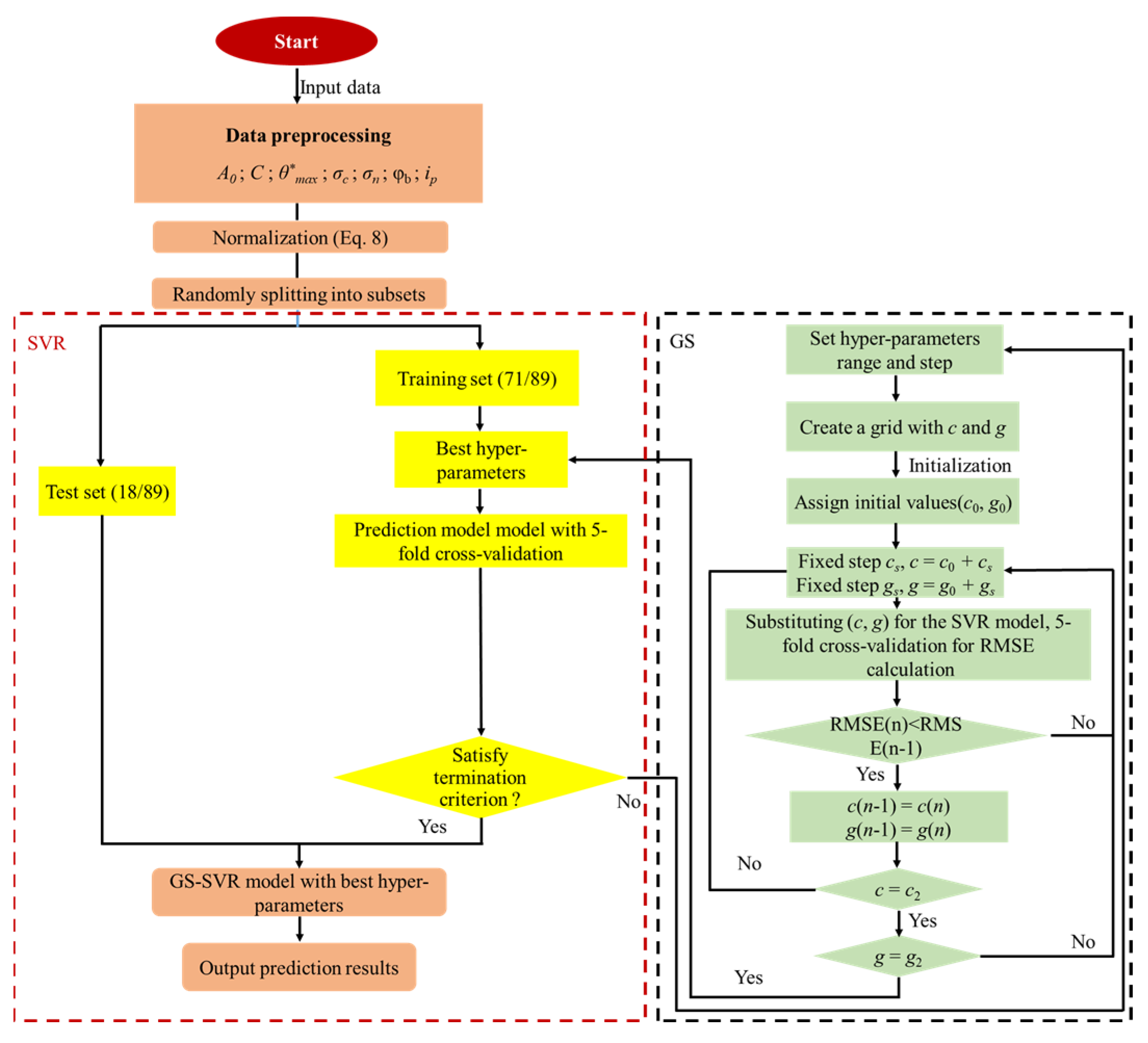
2.1. SVR
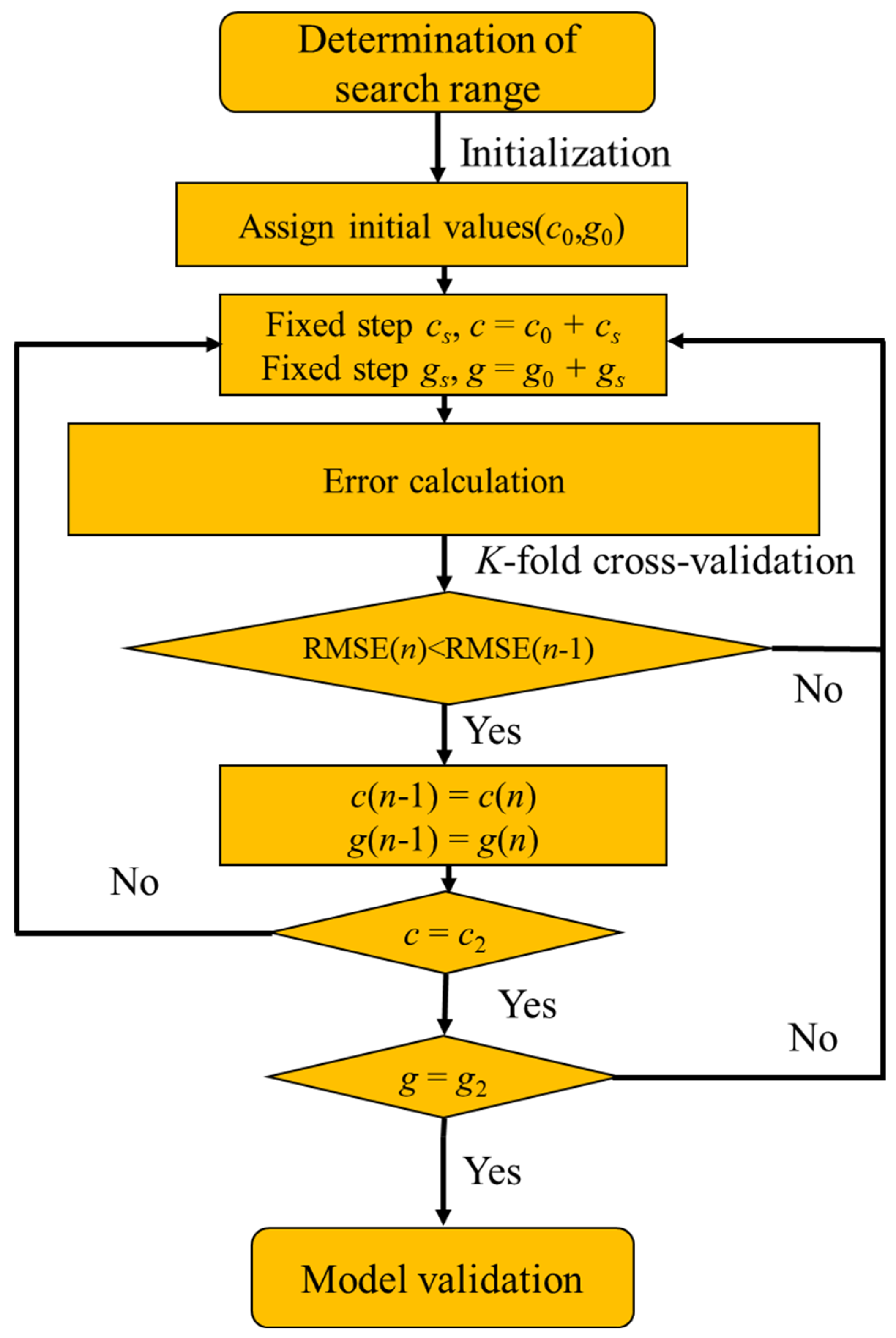
2.2. GS Optimization
3. Data Pre-Processing
4. Results and Comparisons
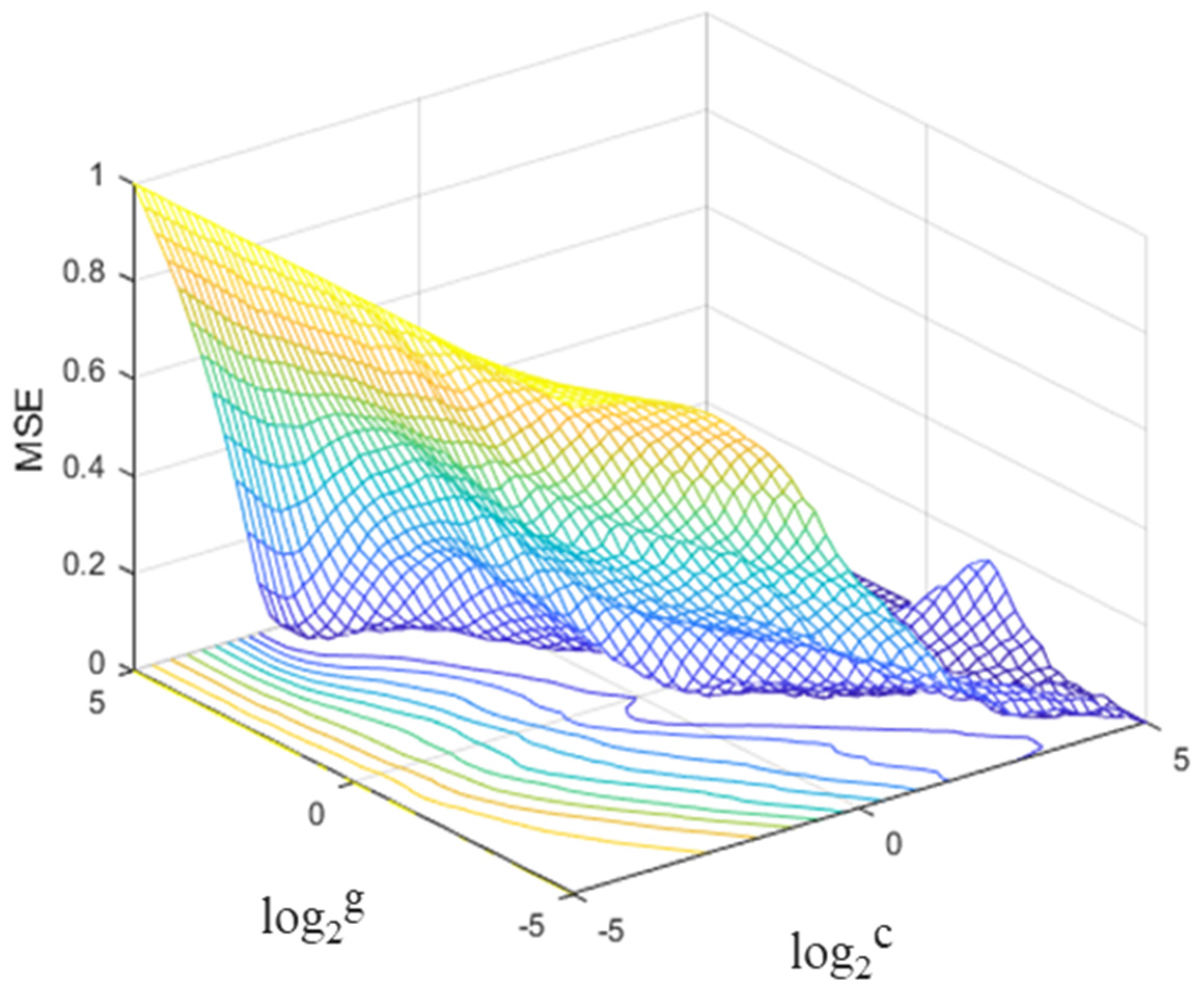
4.1. Hyperparameters Tuning Process
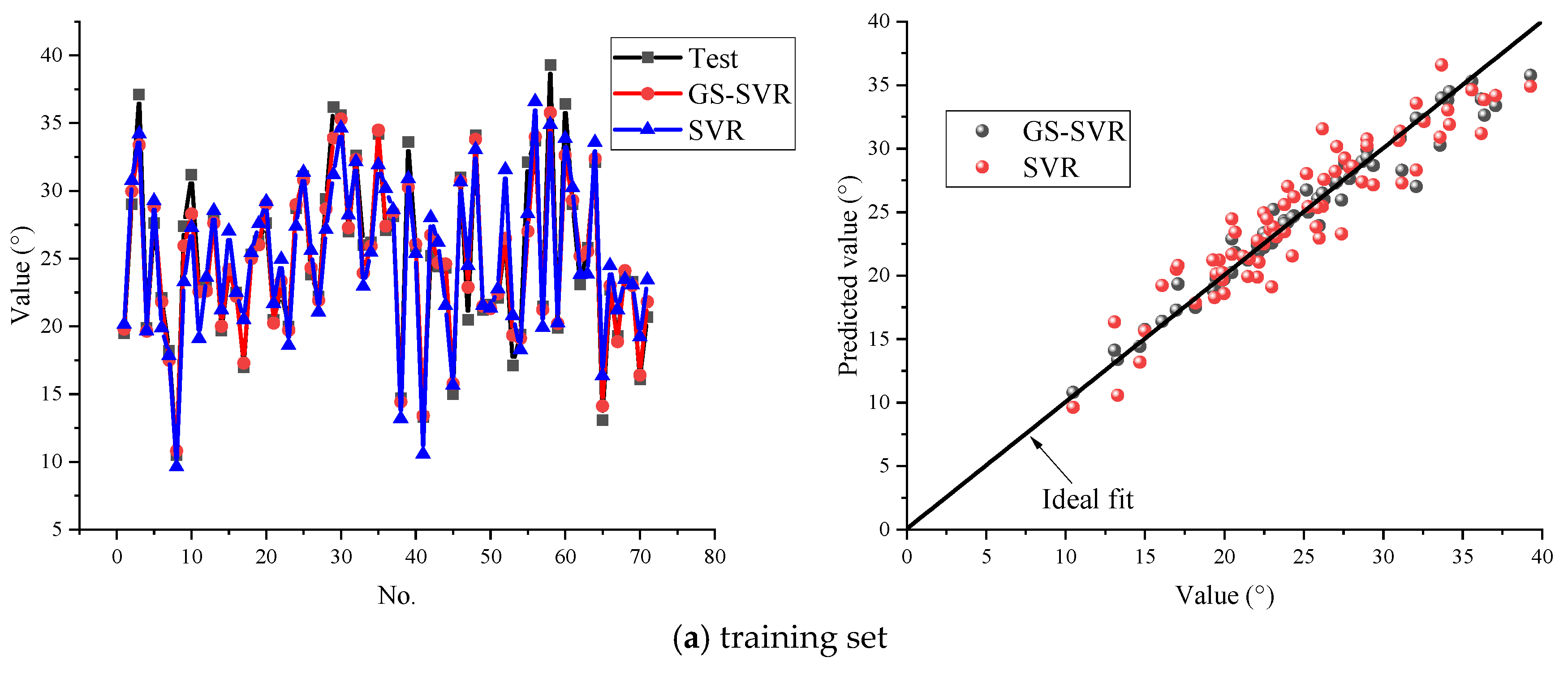
4.2. Performance of GS-SVR Model
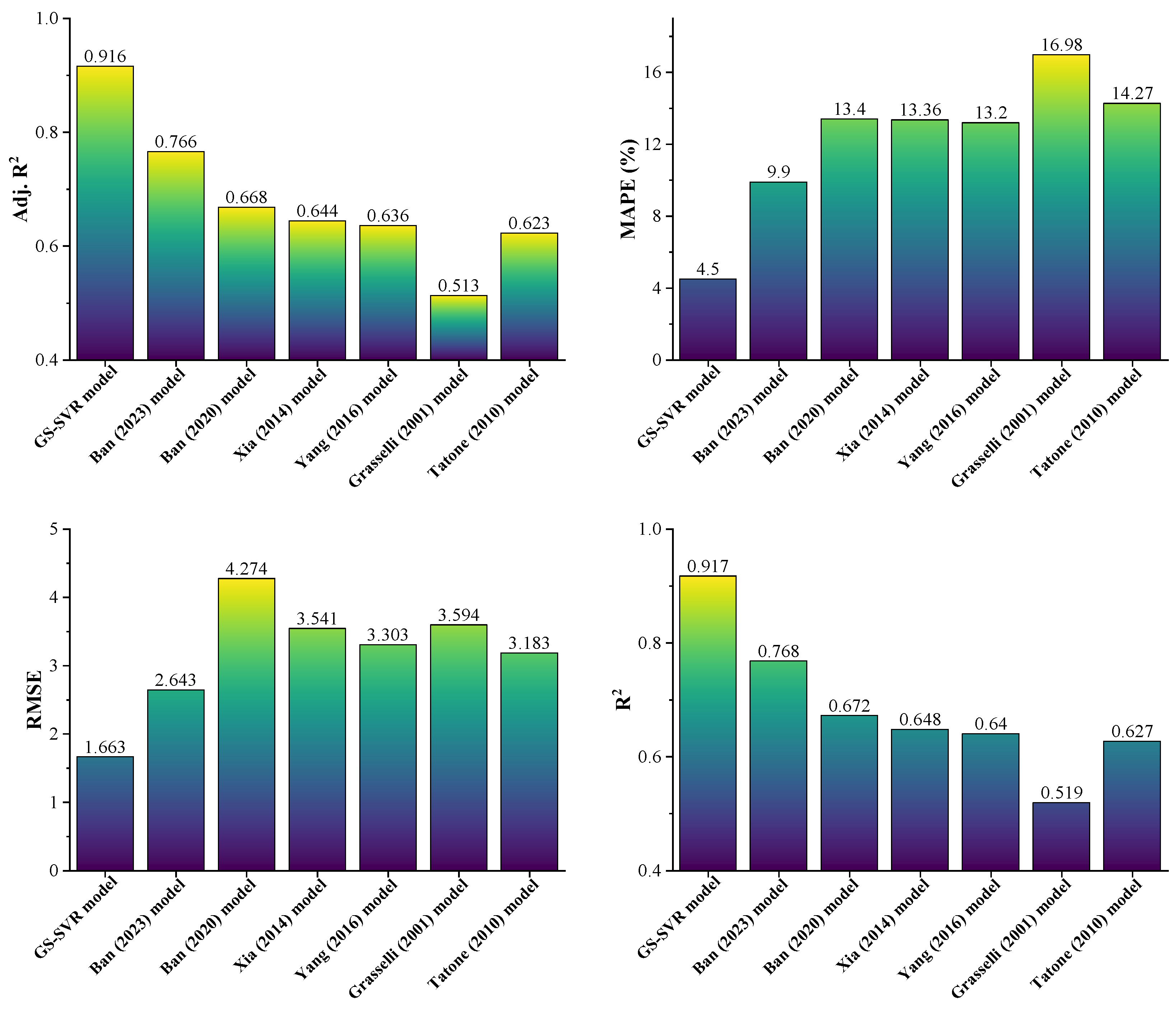
4.3. Comparison with Existing Models
5. Discussion
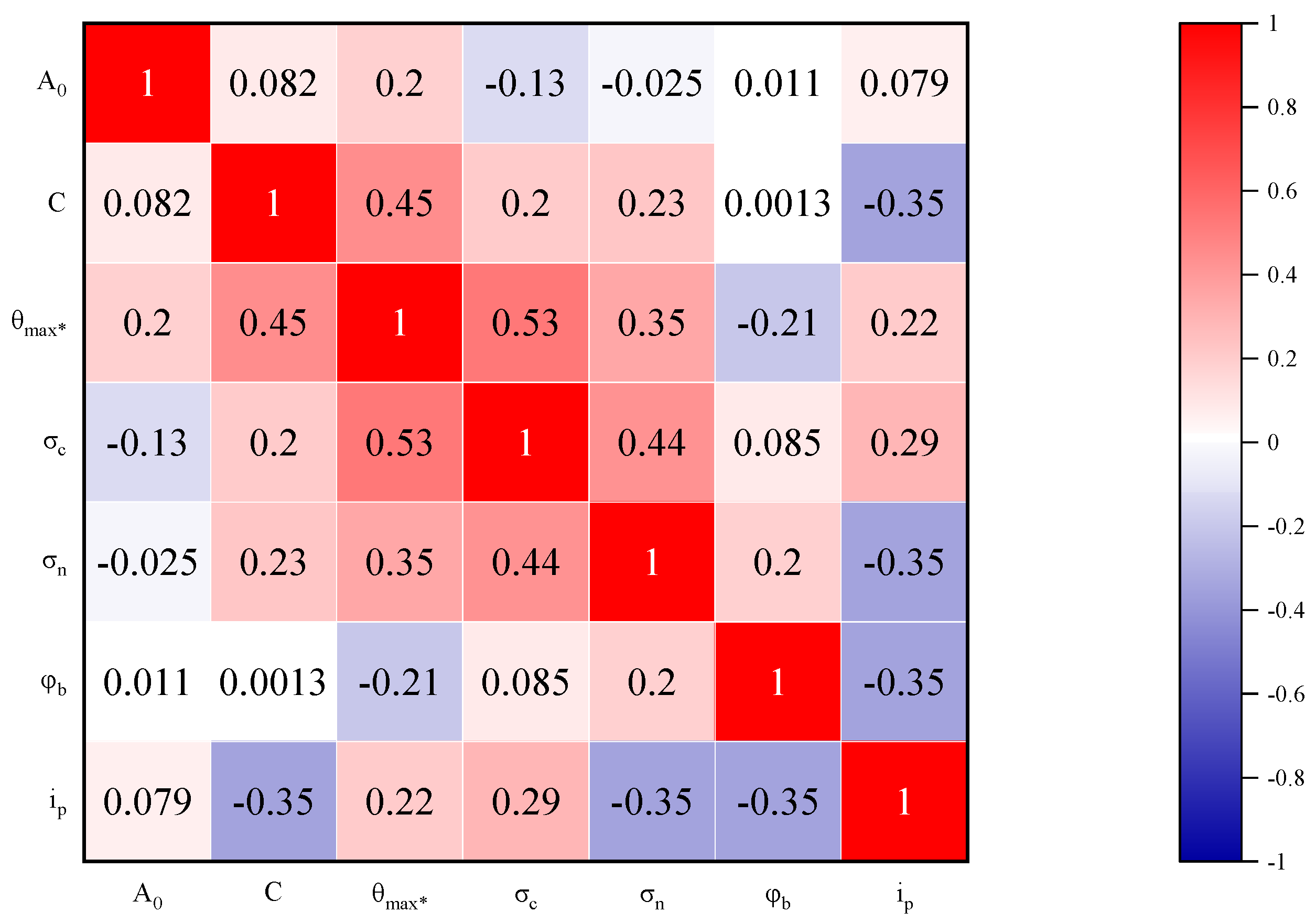
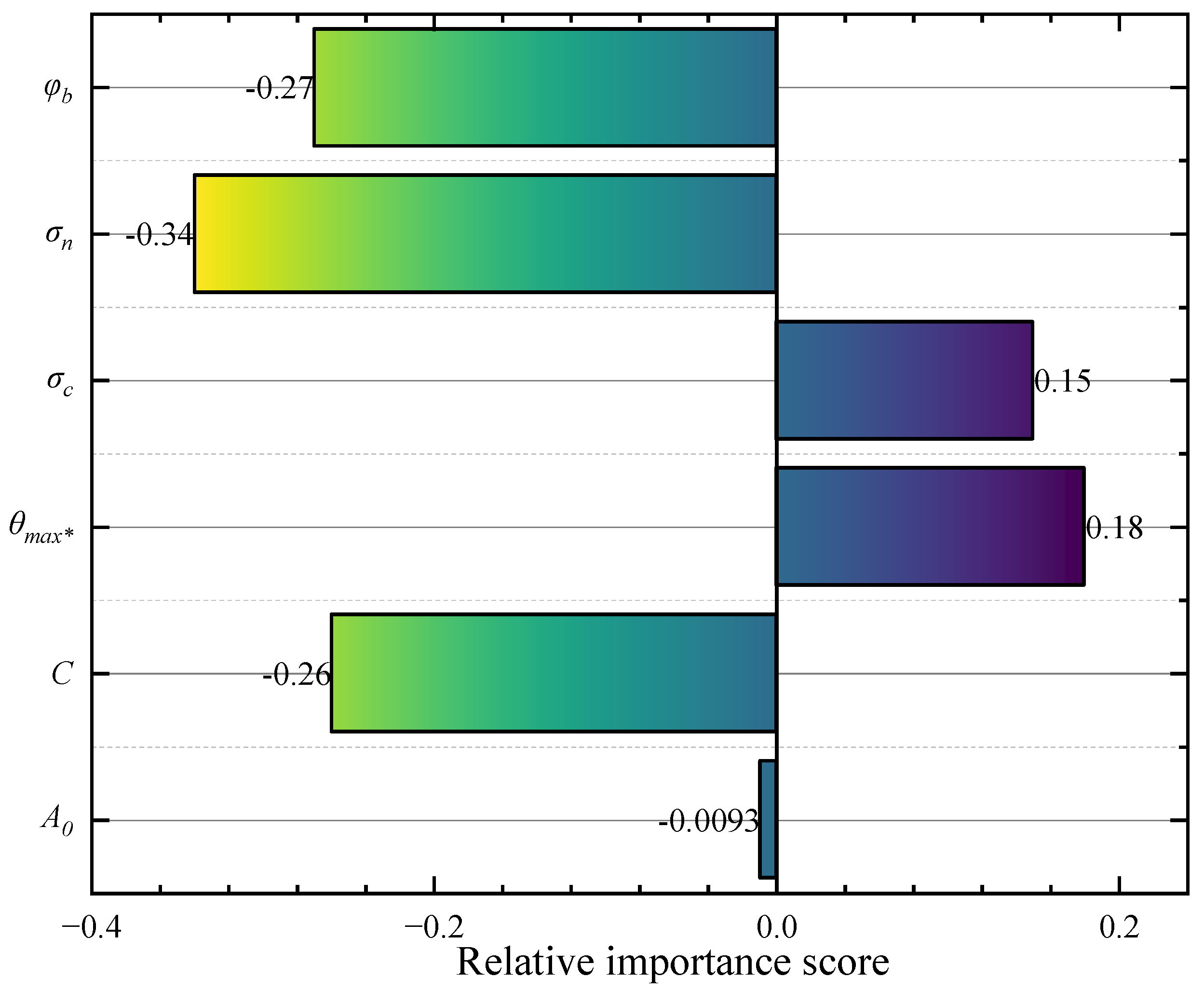
5.1. Relative Importance of Inputs
5.2. Contribution and Limitations
6. Conclusions
Supplementary Materials
Author Contributions
Funding
Data Availability Statement
Conflicts of Interest
Abbreviations
| τp | Shear strength |
| ip | Peak dilation angle |
| i0 | Dilation angle under zero normal stress (°) |
| φb | Basic friction angle |
| k1k2 | Fitting constant |
| SRP | Stationary roughness profile |
| p, q | Regression coefficients |
| C | Roughness parameter characterizing distribution of apparent dip angles over joint surface |
| θA | Average angle of asperities facing shear direction |
| JRC | Joint roughness coefficient |
| JCS | Joint wall compressive strength |
| σn | Normal stress |
| σc | Uniaxial compressive strength |
| a, c, d | Fitting constants |
| σt | Tension strength |
| A0 | Maximum potential contact area for the specified shear direction |
| θmax | Maximum apparent dip angle (°) |
| Average of the mean profile angles | |
| Fitting constant |
References
- Liu, J.; Zhao, Y.; Tan, T.; Zhang, L.; Zhu, S.; Xu, F. Evolution and modeling of mine water inflow and hazard characteristics in southern coalfields of China: A case of Meitanba mine. Int. J. Min. Sci. Technol. 2022, 32, 513–524. [Google Scholar] [CrossRef]
- Yu, W.J.; Li, K.; Liu, Z.; An, B.F.; Wang, P.; Wu, H. Mechanical characteristics and deformation control of surrounding rock in weakly cemented siltstone. Environ. Earth Sci. 2021, 80, 337. [Google Scholar] [CrossRef]
- Hu, K.; Zheng, J.; Wu, H.; Jia, Q. Temperature distribution and equipment layout in a deep chamber: A case study of a coal mine substation. Sustainability 2022, 14, 3852. [Google Scholar] [CrossRef]
- Yuan, W.; Cheng, Y.; Min, M.; Wang, X. Study on acoustic emission characteristics during shear deformation of rock structural planes based on particle flow code. Comput. Part. Mech. 2023. [Google Scholar] [CrossRef]
- Lin, H.; Feng, J.J.; Cao, R.H.; Xie, S.J. Comparative analysis of rock damage models based on different distribution functions. Geotech. Geol. Eng. 2022, 40, 301–310. [Google Scholar] [CrossRef]
- Chen, W.; Wan, W.; Zhao, Y.; Peng, W. Experimental study of the crack predominance of rock-like material containing parallel double fissures under uniaxial compression. Sustainability 2020, 12, 5188. [Google Scholar] [CrossRef]
- Niktabar, S.M.M.; Rao, K.S.; Shrivastava, A.K.; Scucka, J. Effect of varying normal stiffness on soft rock joints under cyclic shear loads. Materials 2023, 16, 4272. [Google Scholar] [CrossRef] [PubMed]
- Xie, S.J.; Lin, H.; Chen, Y.F.; Wang, Y.X.; Cao, R.H.; Li, J.T. Statistical damage shear constitutive model of rock joints under seepage pressure. Front. Earth Sci. 2020, 8, 16. [Google Scholar] [CrossRef]
- Li, M.; Lv, H.; Lu, Y.; Wang, D.; Shi, S.; Li, R. Instantaneous discharge characteristics and its methane ignition mechanism of coal mine rock damage. Environ. Sci. Pollut. Res. 2022, 29, 62495–62506. [Google Scholar] [CrossRef]
- Cai, W.; Zhu, H.; Liang, W. Three-dimensional tunnel face extrusion and reinforcement effects of underground excavations in deep rock masses. Int. J. Rock Mech. Min. Sci. 2022, 150, 104999. [Google Scholar] [CrossRef]
- Cai, W.; Zhu, H.; Liang, W. Three-dimensional stress rotation and control mechanism of deep tunneling incorporating generalized Zhang–Zhu strength-based forward analysis. Eng. Geol. 2022, 308, 106806. [Google Scholar] [CrossRef]
- Xie, S.; Lin, H.; Duan, H. A novel criterion for yield shear displacement of rock discontinuities based on renormalization group theory. Eng. Geol. 2023, 314, 107008. [Google Scholar] [CrossRef]
- Develi, K. Computation of direction dependent joint surface parameters through the algorithm of triangular prism surface area method: A theoretical and experimental study. Int. J. Solids Struct. 2020, 202, 895–911. [Google Scholar] [CrossRef]
- Pellet, F.L.; Keshavarz, M.; Boulon, M. Influence of humidity conditions on shear strength of clay rock discontinuities. Eng. Geol. 2013, 157, 33–38. [Google Scholar] [CrossRef]
- Zhao, Y.L.; Liu, Q.; Zhang, C.S.; Liao, J.; Lin, H.; Wang, Y.X. Coupled seepage-damage effect in fractured rock masses: Model development and a case study. Int. J. Rock Mech. Min. Sci. 2021, 144, 104822. [Google Scholar] [CrossRef]
- Xin, J.; Jiang, Q.; Li, S.; Chen, P.; Zhao, H. Fracturing and energy evolution of rock around prefabricated rectangular and circular tunnels under shearing load: A comparative analysis. Rock Mech. Rock Eng. 2023. [Google Scholar] [CrossRef]
- Shaunik, D.; Singh, M. Bearing capacity of foundations on rock slopes intersected by non-persistent discontinuity. Int. J. Min. Sci. Technol. 2020, 30, 669–674. [Google Scholar] [CrossRef]
- Bahaaddini, M.; Hagan, P.C.; Mitra, R.; Khosravi, M.H. Experimental and numerical study of asperity degradation in the direct shear test. Eng. Geol. 2016, 204, 41–52. [Google Scholar] [CrossRef]
- Wu, H.; Jia, Q.; Wang, W.; Zhang, N.; Zhao, Y. Experimental test on nonuniform deformation in the tilted strata of a deep coal mine. Sustainability 2021, 13, 13280. [Google Scholar] [CrossRef]
- Peng, Y.; Liu, G.; Wu, L.; Zuo, Q.; Liu, Y.; Zhang, C. Comparative study on tunnel blast-induced vibration for the underground cavern group. Environ. Earth Sci. 2021, 80, 68. [Google Scholar] [CrossRef]
- Yan, Y.-T.; Wang, S.-W. Simulation investigation of mechanical and failure characteristics of jointed rock with different shapes of joint asperities under compression loading. Comput. Part. Mech. 2023, 10, 45–59. [Google Scholar] [CrossRef]
- Liren, B.; Yuhang, H.; Weisheng, D.; Jin, Y.; Chengzhi, Q.; Renliang, S. A new peak dilation angle model for rock joints considering different contribution proportions of actual contact joint asperities to shear strength. J. China Coal Soc. 2023, 1–12. [Google Scholar] [CrossRef]
- Xie, S.; Lin, H.; Chen, Y. New constitutive model based on disturbed state concept for shear deformation of rock joints. Arch. Civ. Mech. Eng. 2022, 23, 26. [Google Scholar] [CrossRef]
- Khayrutdinov, M.M.; Kongar-Syuryun, C.B.; Khayrutdinov, A.M.; Tyulyaeva, Y.S. Improving safety when extracting water-soluble ores by optimizing the parameters of the backfill mass. Occup. Saf. Ind. 2021, 53–59. [Google Scholar] [CrossRef]
- Rybak, J.; Tyulyaeva, Y.; Kongar-Syuryun, C.; Khayrutdinov, A.M.; Akinshin, I. Geomechanical substantiation of parameters of technology for mining salt deposits with a backfill. Min. Sci. 2021, 28, 19–32. [Google Scholar] [CrossRef]
- Tang, Z.; Xia, C.; Song, Y. New peak shear strength criteria for roughness joints. Chin. J. Geotech. Eng. 2013, 35, 571–577. [Google Scholar]
- Yuan, W.; Min, M. Investigation on the scale dependence of shear mechanical behavior of rock joints using DEM simulation. Comput. Part. Mech. 2023. [Google Scholar] [CrossRef]
- Nguyen, V.-M.; Konietzky, H.; Frühwirt, T. New methodology to characterize shear behavior of joints by combination of direct shear box testing and numerical simulations. Geotech. Geol. Eng. 2014, 32, 829–846. [Google Scholar] [CrossRef]
- Cai, W.; Zhu, H.; Liang, W.; Wang, X.; Su, C.; Wei, X. A post-peak dilatancy model for soft rock and its application in deep tunnel excavation. J. Rock Mech. Geotech. 2023, 15, 683–701. [Google Scholar] [CrossRef]
- Zhao, Y.L.; Zhang, C.S.; Wang, Y.X.; Lin, H. Shear-related roughness classification and strength model of natural rock joint based on fuzzy comprehensive evaluation. Int. J. Rock Mech. Min. Sci. 2021, 137, 104550. [Google Scholar] [CrossRef]
- Yuan, Z.; Zhao, J.; Li, S.; Jiang, Z.; Huang, F. A unified solution for surrounding rock of roadway considering seepage, dilatancy, strain-softening and intermediate principal stress. Sustainability 2022, 14, 8099. [Google Scholar] [CrossRef]
- Wang, F.; Xie, H.; Zhou, C.; Wang, Z.; Li, C. Combined effects of fault geometry and roadway cross-section shape on the collapse behaviors of twin roadways: An experimental investigation. Tunn. Undergr. Space Technol. 2023, 137, 105106. [Google Scholar] [CrossRef]
- Cai, W.; Su, C.; Zhu, H.; Liang, W.; Ma, Y.; Xu, J.; Xu, C. Elastic–plastic response of a deep tunnel excavated in 3D Hoek–Brown rock mass considering different approaches for obtaining the out-of-plane stress. Int. J. Rock Mech. Min. Sci. 2023, 169, 105425. [Google Scholar] [CrossRef]
- Xie, S.; Lin, H.; Cheng, C.; Chen, Y.; Wang, Y.; Zhao, Y.; Yong, W. Shear strength model of joints based on Gaussian smoothing method and macro-micro roughness. Comput. Geotech. 2022, 143, 104605. [Google Scholar] [CrossRef]
- Ding, L.; Li, G. Research on peak shear strength criterion of rock joints based on the evolution of dilation angle. Geotech. Geol. Eng. 2021, 39, 4887–4900. [Google Scholar] [CrossRef]
- Ladanyi, B.; Archambault, G. (Eds). In Simulation of shear behavior of a jointed rock mass. In Proceedings of the 11th US Symposium on Rock Mechanics (USRMS), Berkeley, CA, USA, 16 June 1969; OnePetro: Richardson, TX, USA, 1969. [Google Scholar]
- Schneider, H. The friction and deformation behaviour of rock joints. Rock Mech. 1976, 8, 169–184. [Google Scholar] [CrossRef]
- Xia, C.-C.; Tang, Z.-C.; Xiao, W.-M.; Song, Y.-L. New peak shear strength criterion of rock joints based on quantified surface description. Rock Mech. Rock Eng. 2014, 47, 387–400. [Google Scholar] [CrossRef]
- Yang, J.; Rong, G.; Hou, D.; Peng, J.; Zhou, C. Experimental study on peak shear strength criterion for rock joints. Rock Mech. Rock Eng. 2016, 49, 821–835. [Google Scholar] [CrossRef]
- Ban, L.; Du, W.; Qi, C. A peak dilation angle model considering the real contact area for rock joints. Rock Mech. Rock Eng. 2020, 53, 4909–4923. [Google Scholar] [CrossRef]
- Barton, N. Review of a new shear-strength criterion for rock joints. Eng. Geol. 1973, 7, 287–332. [Google Scholar] [CrossRef]
- Jing, L.; Nordlund, E.; Stephansson, O. An experimental study on the anisotropy and stress-dependency of the strength and deformability of rock joints. Int. J. Rock Mech. Min. Sci. 1992, 29, 535–542. [Google Scholar] [CrossRef]
- Kulatilake, P.; Shou, G.; Huang, T.; Morgan, R. New peak shear strength criteria for anisotropic rock joints. Int. J. Rock Mech. Min. Sci. 1995, 32, 673–697. [Google Scholar] [CrossRef]
- Ghazvinian, A.H.; Taghichian, A.; Hashemi, M.; Mar’ashi, S.A. The shear behavior of bedding planes of weakness between two different rock types with high strength difference. Rock Mech. Rock Eng. 2010, 43, 69–87. [Google Scholar] [CrossRef]
- Ghazvinian, A.H.; Azinfar, M.J.; Geranmayeh Vaneghi, R. Importance of tensile strength on the shear behavior of discontinuities. Rock Mech. Rock Eng. 2012, 45, 349–359. [Google Scholar] [CrossRef]
- Tang, Z.-C.; Liu, Q.-S.; Huang, J.-H. New criterion for rock joints based on three-dimensional roughness parameters. J. Cent. South Univ. 2014, 21, 4653–4659. [Google Scholar] [CrossRef]
- Kumar, R.; Verma, A.K. Anisotropic shear behavior of rock joint replicas. Int. J. Rock Mech. Min. Sci. 2016, 90, 62–73. [Google Scholar] [CrossRef]
- Cao, P.; Long, L.; Fan, W.; Fan, X.; Cao, R. Peak shear strength criterion for rock joints based on undulating characteristics. J. Cent. South Univ. 2017, 48, 1081–1087. [Google Scholar]
- Zhao, Y.L.; Tang, J.Z.; Chen, Y.; Zhang, L.Y.; Wang, W.J.; Wan, W.; Liao, J.P. Hydromechanical coupling tests for mechanical and permeability characteristics of fractured limestone in complete stress-strain process. Environ. Earth Sci. 2017, 76, 24. [Google Scholar] [CrossRef]
- Zhao, Y.L.; Luo, S.L.; Wang, Y.X.; Wang, W.J.; Zhang, L.Y.; Wan, W. Numerical analysis of karst water inrush and a criterion for establishing the width of water-resistant rock pillars. Mine Water Environ. 2017, 36, 508–519. [Google Scholar] [CrossRef]
- Peng, K.; Yi, G.; Wang, Y.; Luo, S.; Wu, H. Experimental and theoretical analysis of spalling in deep hard rock tunnels with different arch structures. Theor. Appl. Fract. Mech. 2023, 127, 104054. [Google Scholar] [CrossRef]
- Luo, S.; Gong, F.; Peng, K.; Liu, Z. Influence of water on rockburst proneness of sandstone: Insights from relative and absolute energy storage. Eng. Geol. 2023, 323, 107172. [Google Scholar] [CrossRef]
- Xie, S.J.; Lin, H.; Wang, Y.X.; Chen, Y.F.; Xiong, W.; Zhao, Y.L.; Du, S.G. A statistical damage constitutive model considering whole joint shear deformation. Int. J. Damage Mech. 2020, 29, 988–1008. [Google Scholar] [CrossRef]
- Xie, S.J.; Lin, H.; Chen, Y.F.; Wang, Y.X. A new nonlinear empirical strength criterion for rocks under conventional triaxial compression. J. Cent. South Univ. 2021, 28, 1448–1458. [Google Scholar] [CrossRef]
- Xie, S.; Lin, H.; Chen, Y.; Duan, H.; Liu, H.; Liu, B. Prediction of shear strength of rock fractures using support vector regression and grid search optimization. Mater. Today Commun. 2023, 36, 106780. [Google Scholar] [CrossRef]
- Jaskowiec, K.; Wilk-Kolodziejczyk, D.; Bartlomiej, S.; Reczek, W.; Bitka, A.; Malysza, M.; Doroszewski, M.; Pirowski, Z.; Boron, L. Assessment of the quality and mechanical parameters of castings using machine learning methods. Materials 2022, 15, 2884. [Google Scholar] [CrossRef] [PubMed]
- Sun, Z.; Li, Y.; Li, Y.; Su, L.; He, W. Prediction of chloride ion concentration distribution in basalt-polypropylene fiber reinforced concrete based on optimized machine learning algorithm. Mater. Today Commun. 2023, 36, 106565. [Google Scholar] [CrossRef]
- Sun, Z.; Niu, D.; Luo, D.; Wang, X.; Zhang, L.; Su, L.; Li, Y. Hybrid machine learning-based prediction model for the bond strength of corroded Cr alloy-reinforced coral aggregate concrete. Mater. Today Commun. 2023, 35, 106141. [Google Scholar] [CrossRef]
- Wu, Y.; Wang, Y.; Li, D.; Zhang, J. Two-step detection of concrete internal condition using array ultrasound and deep learning. NDT E Int. 2023, 139, 102945. [Google Scholar] [CrossRef]
- Zhang, H.; Su, Y.; Li, A.; Guo, P. Experimental investigation of novel pre-compressed viscoelastic dampers with different matrix materials. Structures 2023, 53, 625–641. [Google Scholar] [CrossRef]
- Xu, G.; Guo, T.; Li, A.Q.; Zhang, H.Y. Self-centering beam-column joints with variable stiffness for steel moment resisting frame. Eng. Struct. 2023, 278, 115526. [Google Scholar] [CrossRef]
- Garcia-Gonzalo, E.; Fernandez-Muniz, Z.; Nieto, P.J.G.; Sanchez, A.B.; Fernandez, M.M. Hard-rock stability analysis for span design in entry-type excavations with learning classifiers. Materials 2016, 9, 531. [Google Scholar] [CrossRef]
- Fakhri, D.; Mahmoodzadeh, A.; Hussein Mohammed, A.; Khodayari, A.; Hashim Ibrahim, H.; Rashidi, S.; Taher Karim, S.H. Forecasting failure load of Sandstone under different Freezing-Thawing cycles using Gaussian process regression method and grey wolf optimization algorithm. Theor. Appl. Fract. Mec. 2023, 125, 103876. [Google Scholar] [CrossRef]
- Chen, J.; Huang, H.; Cohn, A.G.; Zhang, D.; Zhou, M. Machine learning-based classification of rock discontinuity trace: SMOTE oversampling integrated with GBT ensemble learning. Int. J. Min. Sci. Technol. 2022, 32, 309–322. [Google Scholar] [CrossRef]
- Sun, Z.; Wang, L.; Zhou, J.-Q.; Wang, C. A new method for determining the hydraulic aperture of rough rock fractures using the support vector regression. Eng. Geol. 2020, 271, 105618. [Google Scholar] [CrossRef]
- Huang, J.; Zhang, J.; Gao, Y. Intelligently predict the rock joint shear strength using the support vector regression and firefly algorithm. Lithosphere 2021, 2021, 2467126. [Google Scholar] [CrossRef]
- Babanouri, N.; Fattahi, H. Constitutive modeling of rock fractures by improved support vector regression. Environ. Earth Sci. 2018, 77, 243. [Google Scholar] [CrossRef]
- Ceryan, N.; Ozkat, E.C.; Can, N.K.; Ceryan, S. Machine learning models to estimate the elastic modulus of weathered magmatic rocks. Environ. Earth Sci. 2021, 80, 448. [Google Scholar] [CrossRef]
- Xu, C.; Nait Amar, M.; Ghriga, M.A.; Ouaer, H.; Zhang, X.; Hasanipanah, M. Evolving support vector regression using Grey Wolf optimization; forecasting the geomechanical properties of rock. Eng. Comput. 2022, 38, 1819–1833. [Google Scholar] [CrossRef]
- Safari, M.; Rabiee, A.H.; Joudaki, J. Developing a support vector regression (SVR) model for prediction of main and lateral bending angles in laser tube bending process. Materials 2023, 16, 3251. [Google Scholar] [CrossRef]
- Wu, Y.; Zhou, Y. Splitting tensile strength prediction of sustainable high-performance concrete using machine learning techniques. Environ. Sci. Pollut. Res. 2022, 29, 89198–89209. [Google Scholar] [CrossRef]
- Samui, P. Slope stability analysis: A support vector machine approach. Environ. Geol. 2008, 56, 255–267. [Google Scholar] [CrossRef]
- Wu, Y.Q.; Zhou, Y.S. Hybrid machine learning model and Shapley additive explanations for compressive strength of sustainable concrete. Constr. Build. Mater. 2022, 330, 127298. [Google Scholar] [CrossRef]
- Gilan, S.S.; Jovein, H.B.; Ramezanianpour, A.A. Hybrid support vector regression—Particle swarm optimization for prediction of compressive strength and RCPT of concretes containing metakaolin. Constr. Build. Mater. 2012, 34, 321–329. [Google Scholar] [CrossRef]
- Al-Sodani, K.A.A.; Adewumi, A.A.; Ariffin, M.A.M.; Maslehuddin, M.; Ismail, M.; Salami, H.O.; Owolabi, T.O.; Mohamed, H.D. Experimental and modelling of alkali-activated mortar compressive strength using hybrid support vector regression and genetic algorithm. Materials 2021, 14, 3049. [Google Scholar] [CrossRef]
- Anton, C.; Curteanu, S.; Lisa, C.; Leon, F. Machine learning methods applied for modeling the process of obtaining bricks using silicon-based materials. Materials 2021, 14, 7232. [Google Scholar] [CrossRef]
- Muhammad; Kennedy, J.; Lim, C.W. Machine learning and deep learning in phononic crystals and metamaterials—A review. Mater. Today Commun. 2022, 33, 104606. [Google Scholar] [CrossRef]
- Chen, J.; Zhou, M.; Huang, H.; Zhang, D.; Peng, Z. Automated extraction and evaluation of fracture trace maps from rock tunnel face images via deep learning. Int. J. Rock Mech. Min. Sci. 2021, 142, 104745. [Google Scholar] [CrossRef]
- Grasselli, G. Shear Strength of Rock Joints Based on Quantified Surface Description; EPFL: Lausanne, Switzerland, 2001. [Google Scholar]
- Tatone, B.S.A.; Grasselli, G. A method to evaluate the three-dimensional roughness of fracture surfaces in brittle geomaterials. Rev. Sci. Instrum. 2009, 80, 125110. [Google Scholar] [CrossRef]
- Lei, Y.; Zhou, S.; Luo, X.; Niu, S.; Jiang, N. A comparative study of six hybrid prediction models for uniaxial compressive strength of rock based on swarm intelligence optimization algorithms. Front. Earth Sci. 2022, 10, 930130. [Google Scholar] [CrossRef]
- Xie, S.; Lin, H.; Duan, H.; Chen, Y. Modeling description of interface shear deformation: A theoretical study on damage statistical distributions. Constr. Build. Mater. 2023, 394, 132052. [Google Scholar] [CrossRef]


| References | Shear Strength Model | Peak Dilation Angle |
|---|---|---|
| [41] | ||
| [37] | ||
| [42] | ||
| [43] | ||
| [44] | ||
| [45] | ||
| [38] | ||
| [46] | ||
| [47] | ||
| [39] | ||
| [48] | ||
| [40] | / | |
| [22] | / |
| Variables | Type | Maximum | Minimum | Mean | Standard Deviation | Kurtosis | Skewness |
|---|---|---|---|---|---|---|---|
| A0 | Input | 0.69 | 0.43 | 0.51517 | 0.05727 | 2.76052 | 1.54207 |
| C | Input | 13 | 3.21 | 8.12258 | 2.18752 | −0.36112 | −0.43657 |
| θmax* (°) | Input | 90 | 39 | 68.11685 | 12.15342 | −0.65228 | −0.30474 |
| σc (MPa) | Input | 173 | 10 | 64.52247 | 54.23245 | −0.33911 | 1.08714 |
| σn (MPa) | Input | 8 | 0.2 | 1.95169 | 1.48853 | 4.13201 | 1.80875 |
| φb (°) | Input | 37 | 28 | 33.53933 | 2.64169 | −0.13365 | −0.66941 |
| ip (°) | Output | 39.3 | 8.5 | 24.89888 | 6.32154 | −0.02348 | −0.1438 |
| Model | Training Set | Test Set | ||||||
|---|---|---|---|---|---|---|---|---|
| R2 | Adj. R2 | RMSE | MAPE | R2 | Adj. R2 | RMSE | MAPE | |
| GS-SVR | 0.959 | 0.959 | 1.138 | 3.1% | 0.891 | 0.884 | 1.798 | 10.8% |
| SVR | 0.868 | 0.866 | 2.102 | 7.8% | 0.780 | 0.767 | 3.237 | 12.7% |
| Rock Type | Peak Dilation Angle (°) | |||||||
|---|---|---|---|---|---|---|---|---|
| Measured | GS-SVR Model | Ban (2023) Model [22] | Ban (2020) Model [40] | Xia (2014) Model [38] | Yang (2016) Model [39] | Grasselli (2001) Model [79] | Tatone (2010) Model [80] | |
| Sandstone [80] | 36.4 | 32.63 | 32.4 | 33.2 | 33 | 24.5 | 33.8 | 33.6 |
| 32.1 | 32.39 | 31.7 | 31.7 | 30.2 | 24.6 | 31.2 | 31.6 | |
| 31.1 | 30.82 | 28.9 | 29.1 | 27.3 | 23.3 | 28.8 | 29.2 | |
| 30.3 | 27.30 | 30.4 | 30.3 | 27.3 | 24.8 | 27.6 | 28.6 | |
| 28.5 | 25.85 | 29 | 29.3 | 25.7 | 24.4 | 26.1 | 27.1 | |
| 27.6 | 29.01 | 27.2 | 27.1 | 23.1 | 22.9 | 24.2 | 25 | |
| Sandstone [38] | 24.6 | 18.32 | 19.7 | 19.7 | 17.3 | 18.4 | 22 | 22.4 |
| 15 | 15.75 | 17 | 17 | 15.1 | 16.6 | 18.1 | 18.8 | |
| 14.7 | 14.41 | 15.4 | 15.4 | 13.6 | 14.9 | 15.1 | 15.8 | |
| 13.3 | 13.38 | 14.2 | 14.2 | 12.6 | 13.4 | 12.8 | 13.6 | |
| 8.5 | 8.44 | 12.4 | 12.4 | 11.4 | 10.9 | 10.1 | 10.7 | |
| 31.2 | 28.29 | 28.5 | 28.6 | 24.5 | 24.9 | 24.5 | 25.1 | |
| 25.3 | 25.0 | 24.9 | 24.9 | 20.7 | 22.9 | 19.9 | 20.8 | |
| 20.7 | 21.80 | 22.6 | 22.6 | 18.5 | 21 | 16.9 | 17.8 | |
| 19.3 | 18.85 | 20.9 | 20.9 | 17.2 | 19.2 | 15.1 | 15.8 | |
| 13.1 | 14.09 | 18.4 | 18.4 | 16.1 | 16.2 | 13.5 | 13.9 | |
| 39.3 | 35.78 | 31.2 | 31.4 | 36.9 | 25.6 | 26.5 | 27 | |
| 32.6 | 32.31 | 27.7 | 27.8 | 31.9 | 23.6 | 22.6 | 23.4 | |
| 27.6 | 28.81 | 25.5 | 25.5 | 28.6 | 21.7 | 19.6 | 20.5 | |
| 25.4 | 20.54 | 23.8 | 23.8 | 26.4 | 20 | 17.5 | 18.4 | |
| 19.5 | 19.78 | 21.3 | 21.3 | 24.1 | 17 | 15.2 | 15.8 | |
| Sandstone [39] | 37.1 | 33.40 | 28.3 | 38.9 | 29 | 29 | 29 | 29 |
| 26.2 | 26.48 | 28.2 | 39.9 | 38.6 | 31.5 | 29 | 29 | |
| 29 | 29.29 | 29.9 | 34.5 | 29 | 29 | 25.2 | 25.2 | |
| 29 | 29.96 | 28.6 | 31.2 | 22.9 | 27.6 | 22.9 | 22.9 | |
| 24.3 | 24.59 | 27.1 | 28.6 | 24.3 | 26.8 | 21.5 | 19.9 | |
| 29 | 22.47 | 28.8 | 31.8 | 27.2 | 28.1 | 21.7 | 20.5 | |
| 27.4 | 25.95 | 26.2 | 27.5 | 19.7 | 25.8 | 18.6 | 17.3 | |
| 26.2 | 25.91 | 25.5 | 26.7 | 18.1 | 25.4 | 17 | 17 | |
| 24.4 | 24.69 | 23.7 | 24.5 | 15.8 | 24.4 | 15.8 | 14.7 | |
| 27.3 | 21.03 | 25.8 | 27.3 | 19.9 | 25.6 | 17.5 | 16.6 | |
| Marble [79] | 25.9 | 26.06 | 27.5 | 30.2 | 27.2 | 25.9 | 27.2 | 27.2 |
| 16.1 | 16.38 | 20.3 | 20.3 | 20.4 | 17.2 | 24.6 | 24.6 | |
| 17.1 | 19.32 | 23.5 | 23.9 | 19.2 | 21.2 | 25.9 | 25.9 | |
| 19.9 | 20.19 | 20.6 | 20.9 | 21.2 | 19.5 | 22.1 | 22.5 | |
| 22.5 | 22.20 | 20.4 | 20.6 | 21.9 | 18.6 | 23.6 | 23.6 | |
| 21.9 | 20.92 | 20.3 | 20.6 | 17.9 | 20 | 22.5 | 23 | |
| 19 | 19.67 | 19.2 | 19.4 | 19 | 20.4 | 21.2 | 22.1 | |
| 22.1 | 21.80 | 19.2 | 19.4 | 17.7 | 19.6 | 20.9 | 21.7 | |
| 23 | 22.54 | 17.9 | 18 | 17.9 | 17.2 | 22.5 | 22.5 | |
| 22.9 | 22.61 | 24 | 24.4 | 22.9 | 21.2 | 25.9 | 25.9 | |
| 22.2 | 21.91 | 22.8 | 23.1 | 19.5 | 20.4 | 26.6 | 25.3 | |
| 17 | 17.27 | 19.8 | 20.3 | 20.5 | 17 | 14.9 | 17 | |
| 10.5 | 10.78 | 8.4 | 8.4 | 14 | 4.9 | 12.3 | 11.1 | |
| 10.8 | 10.41 | 13.8 | 14 | 16.3 | 9.5 | 29.1 | 13.1 | |
| Granite [79] | 34.1 | 33.81 | 35 | 42.3 | 33 | 35.7 | 29.5 | 30.4 |
| 33.7 | 33.99 | 34.3 | 44.5 | 36.5 | 35.7 | 31.8 | 32.2 | |
| 31.5 | 30.10 | 34.2 | 36.9 | 31.5 | 29 | 29 | 29.6 | |
| 31 | 30.71 | 33.9 | 35.4 | 29.1 | 25.5 | 30.1 | 30.1 | |
| 34.9 | 31.36 | 34.6 | 42.6 | 33.5 | 32.7 | 31 | 31.9 | |
| 34.2 | 34.49 | 34.8 | 42 | 32.7 | 31.9 | 31 | 31.9 | |
| 35.6 | 35.31 | 33 | 44.6 | 38.8 | 32.7 | 32.7 | 33.5 | |
| Granite [39] | 27.9 | 27.63 | 27.6 | 34.2 | 33.2 | 28 | 28 | 28 |
| 28.7 | 28.98 | 27.9 | 32.2 | 28 | 28 | 27.1 | 27.1 | |
| 29.4 | 28.67 | 27.1 | 29.7 | 23.8 | 27.4 | 25.1 | 25.1 | |
| 27.1 | 27.39 | 27 | 29.8 | 24.9 | 27.1 | 24.4 | 24.4 | |
| 24 | 24.18 | 23.8 | 24.8 | 19.5 | 24 | 21.4 | 21.4 | |
| 22.7 | 22.99 | 23.1 | 23.9 | 19.2 | 23.4 | 20.4 | 20.4 | |
| 22.6 | 20.57 | 22.2 | 22.8 | 20 | 22 | 19.6 | 20 | |
| 25.8 | 25.52 | 24.8 | 26.4 | 23.4 | 24.4 | 20 | 20.3 | |
| 23.3 | 23.01 | 23.4 | 24.5 | 19.7 | 23.3 | 18.3 | 18.6 | |
| 23.8 | 24.09 | 25.1 | 27.1 | 22.3 | 24.8 | 19 | 19 | |
| Limestone [79] | 28.1 | 28.39 | 26.9 | 30.5 | 27 | 28.1 | 24.6 | 25.9 |
| 27 | 27.28 | 28 | 35.4 | 28.1 | 31.7 | 28.1 | 28.1 | |
| 20 | 19.70 | 19.7 | 20.4 | 19 | 17.9 | 20 | 19 | |
| 26 | 23.93 | 24.8 | 27.1 | 24.9 | 23.2 | 23.2 | 22.5 | |
| 22.1 | 22.39 | 23.8 | 26.2 | 24.1 | 23.1 | 23.1 | 22.7 | |
| 28.1 | 28.39 | 27.9 | 33.4 | 33.3 | 28.1 | 28.1 | 28.1 | |
| 21.6 | 21.30 | 23.5 | 25.5 | 25.8 | 21.6 | 21.6 | 21.6 | |
| Cement mortar [40] | 33.6 | 30.27 | 24.6 | 24.7 | 25.7 | 21.7 | 24.7 | 25.4 |
| 25.2 | 26.73 | 21.5 | 21.5 | 23.1 | 20 | 20.9 | 21.5 | |
| 22.5 | 23.33 | 19.5 | 19.5 | 21.3 | 18.4 | 17.7 | 18.5 | |
| 20.5 | 20.22 | 18 | 18 | 20 | 17 | 15.5 | 16.3 | |
| 30.3 | 25.53 | 21.5 | 21.5 | 22.9 | 19.6 | 23.6 | 24 | |
| 22.5 | 21.53 | 18.6 | 18.6 | 20.7 | 17.7 | 20 | 20.7 | |
| 21.2 | 21.48 | 16.8 | 16.8 | 19.1 | 16.3 | 16.9 | 17.7 | |
| 19.4 | 19.10 | 15.5 | 15.5 | 18.1 | 15 | 14.7 | 15.5 | |
| 32.1 | 27.02 | 23.8 | 23.9 | 27.9 | 22.1 | 24.7 | 25 | |
| 23.8 | 24.31 | 20.7 | 20.8 | 25.4 | 20 | 21.3 | 21.9 | |
| 21.8 | 20.09 | 18.8 | 18.8 | 23.5 | 18.1 | 18.4 | 19.3 | |
| 19.9 | 19.62 | 17.4 | 17.4 | 22.1 | 16.3 | 16.3 | 17.1 | |
| 26.3 | 26.01 | 22.7 | 22.7 | 27.9 | 20.5 | 24.3 | 24.7 | |
| 20.5 | 22.88 | 19.8 | 19.8 | 25.4 | 18.7 | 21.3 | 21.9 | |
| 19.7 | 19.99 | 18 | 18 | 23.6 | 16.9 | 18.5 | 19.3 | |
| 18.2 | 17.47 | 16.6 | 16.7 | 22.3 | 15.4 | 16.4 | 17.3 | |
| 36.2 | 33.91 | 27.9 | 28.1 | 33.2 | 23.3 | 26.7 | 27 | |
| 27.6 | 25.92 | 24.7 | 24.8 | 29.8 | 21.5 | 22.9 | 23.6 | |
| 23.1 | 25.19 | 22.6 | 22.7 | 27.3 | 20 | 19.9 | 20.7 | |
| 21.5 | 21.21 | 21 | 21.1 | 25.5 | 18.6 | 17.7 | 18.5 | |
Disclaimer/Publisher’s Note: The statements, opinions and data contained in all publications are solely those of the individual author(s) and contributor(s) and not of MDPI and/or the editor(s). MDPI and/or the editor(s) disclaim responsibility for any injury to people or property resulting from any ideas, methods, instructions or products referred to in the content. |
© 2023 by the authors. Licensee MDPI, Basel, Switzerland. This article is an open access article distributed under the terms and conditions of the Creative Commons Attribution (CC BY) license (https://creativecommons.org/licenses/by/4.0/).
Share and Cite
Xie, S.; Yao, R.; Yan, Y.; Lin, H.; Zhang, P.; Chen, Y. Hybrid Machine-Learning-Based Prediction Model for the Peak Dilation Angle of Rock Discontinuities. Materials 2023, 16, 6387. https://doi.org/10.3390/ma16196387
Xie S, Yao R, Yan Y, Lin H, Zhang P, Chen Y. Hybrid Machine-Learning-Based Prediction Model for the Peak Dilation Angle of Rock Discontinuities. Materials. 2023; 16(19):6387. https://doi.org/10.3390/ma16196387
Chicago/Turabian StyleXie, Shijie, Rubing Yao, Yatao Yan, Hang Lin, Peilei Zhang, and Yifan Chen. 2023. "Hybrid Machine-Learning-Based Prediction Model for the Peak Dilation Angle of Rock Discontinuities" Materials 16, no. 19: 6387. https://doi.org/10.3390/ma16196387
APA StyleXie, S., Yao, R., Yan, Y., Lin, H., Zhang, P., & Chen, Y. (2023). Hybrid Machine-Learning-Based Prediction Model for the Peak Dilation Angle of Rock Discontinuities. Materials, 16(19), 6387. https://doi.org/10.3390/ma16196387