
An Inverse Method for Measuring Elastoplastic Properties of Metallic Materials Using Bayesian Model and Residual Imprint from Spherical Indentation


Abstract
:1. Introduction
2. Material and Experiments
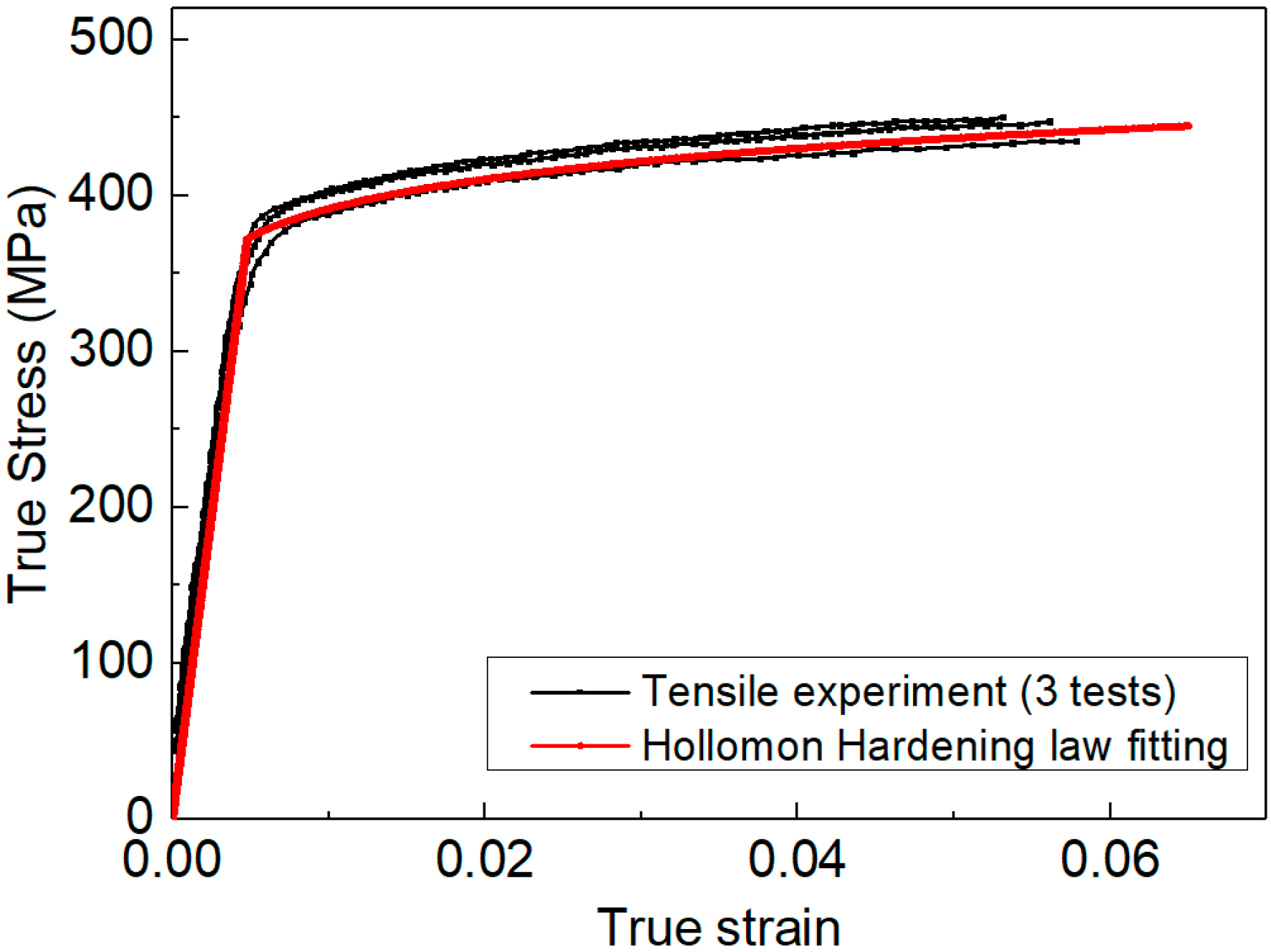
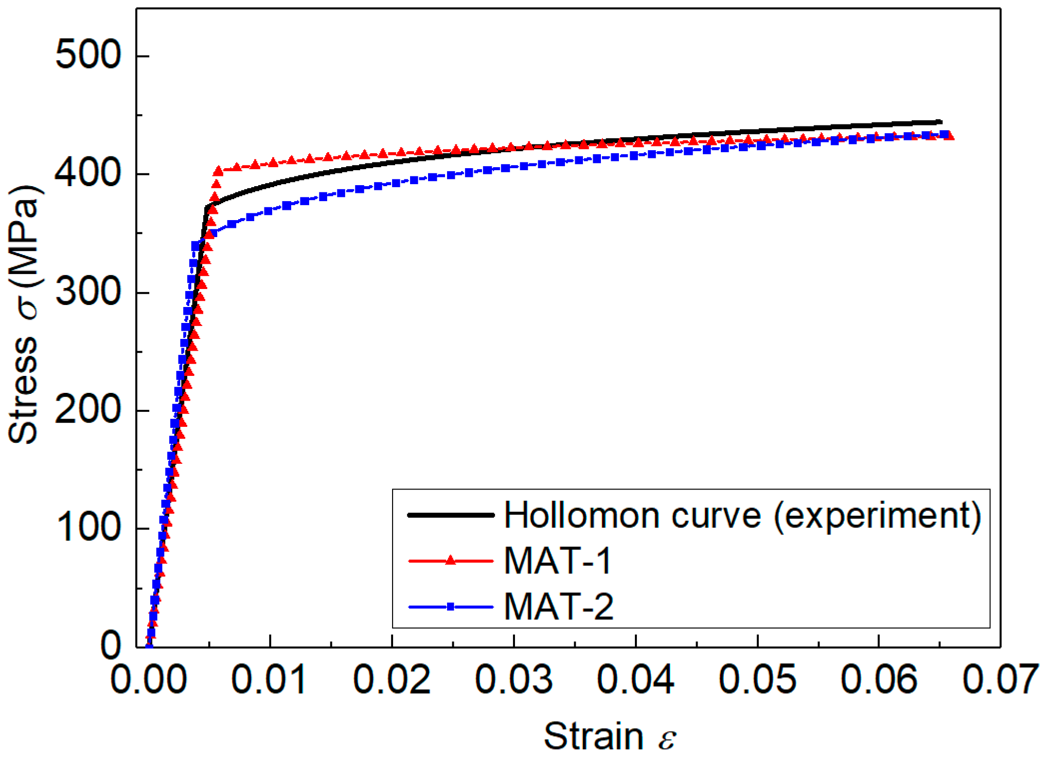
2.1. Material
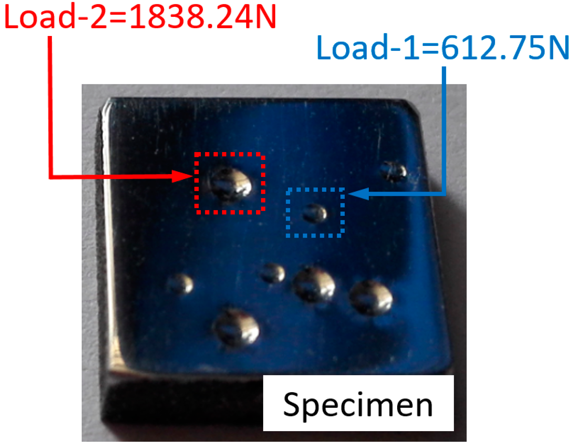
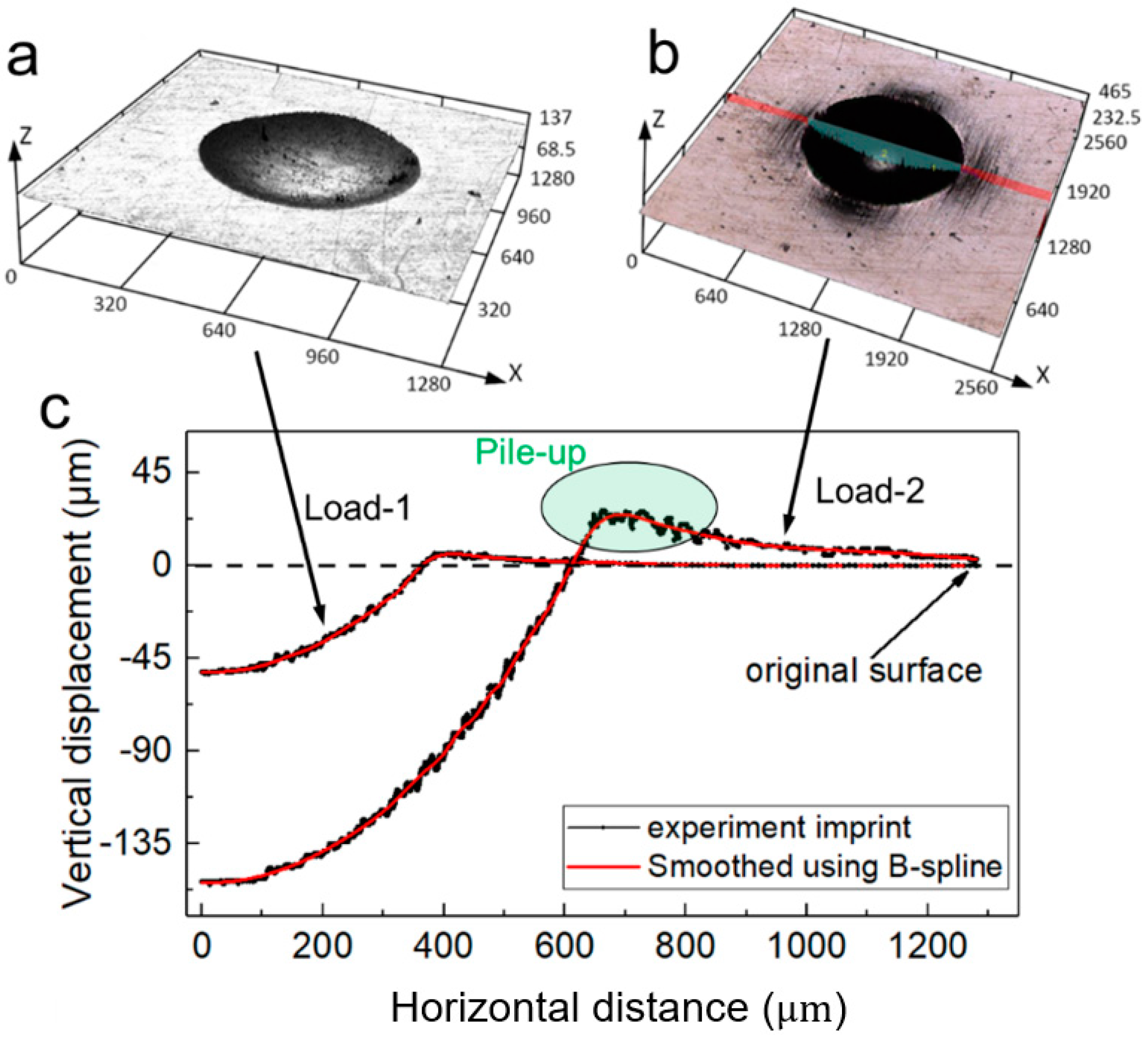
2.2. Indentation Experiment
3. The Basic Methods
3.1. Mathematical Analysis Tools
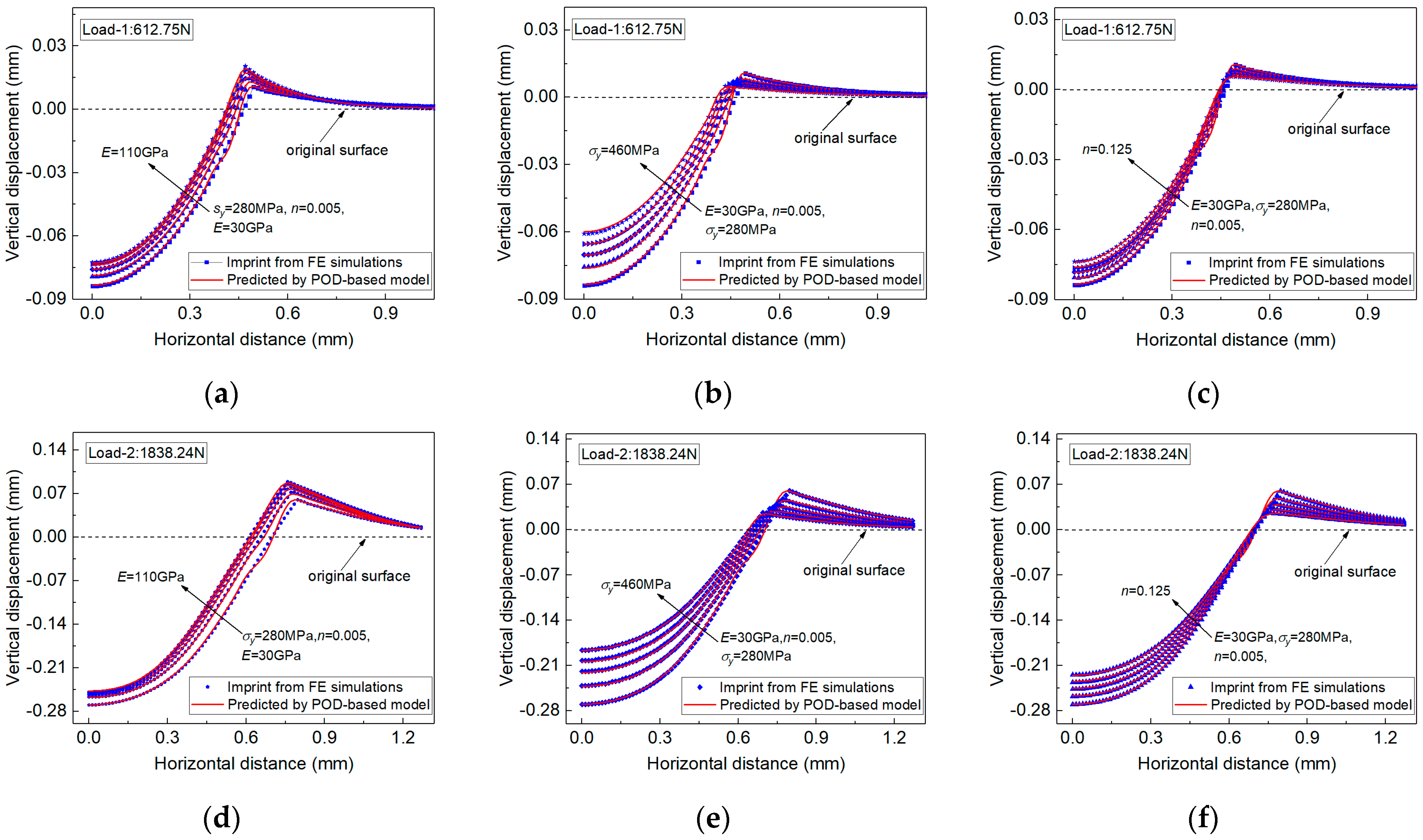
3.1.1. Correlate Elastoplastic Parameters with Indentation Imprint Snapshots Using a POD-Based Numerical Model
3.1.2. Bayesian Inference in Sub-Space of Indentation Imprints
3.1.3. The Proper Weighting in the Sub-Space of Indentation Imprint Snapshots
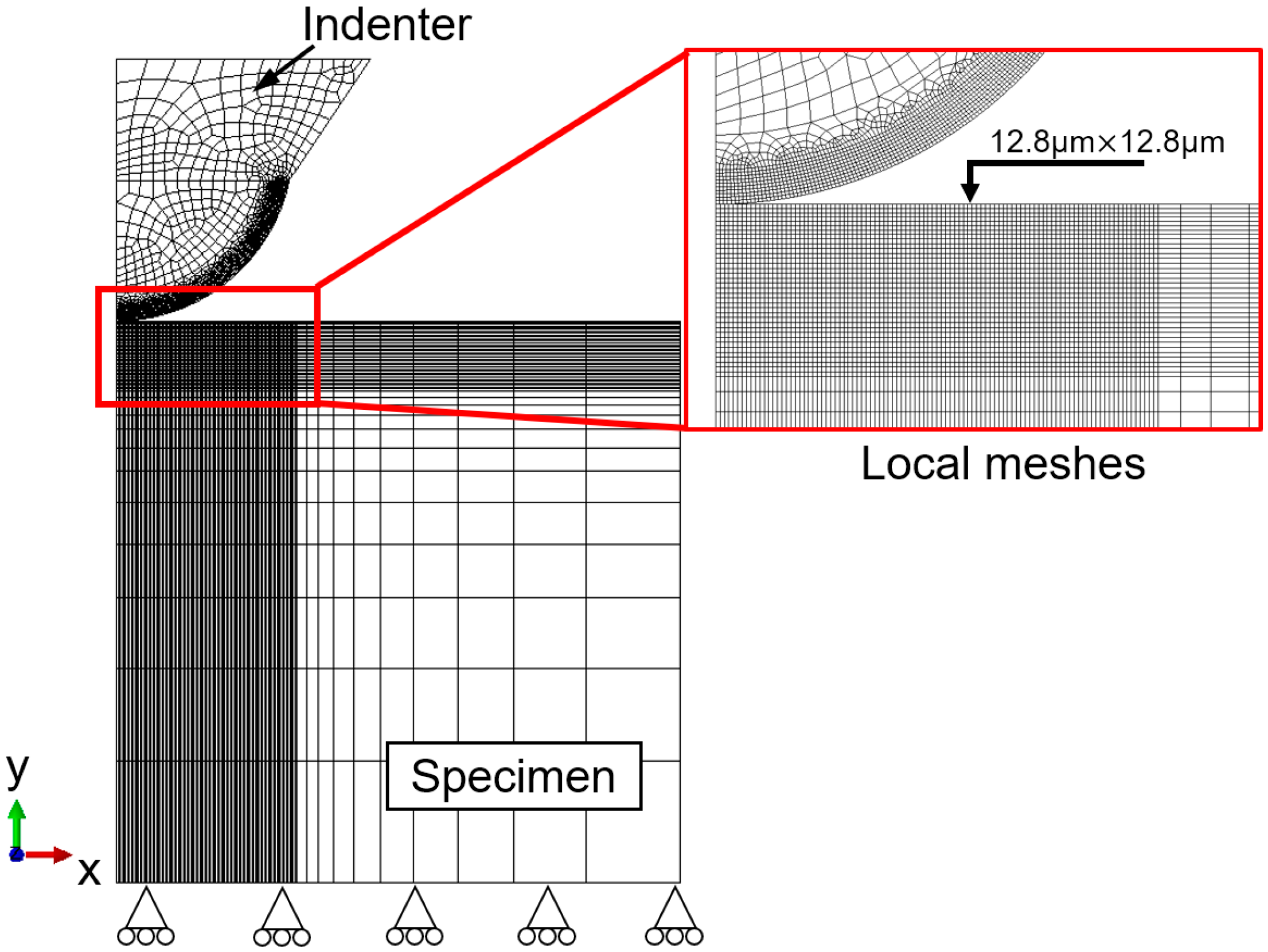
3.2. Finite Element Simulation of Spherical Indentation Test
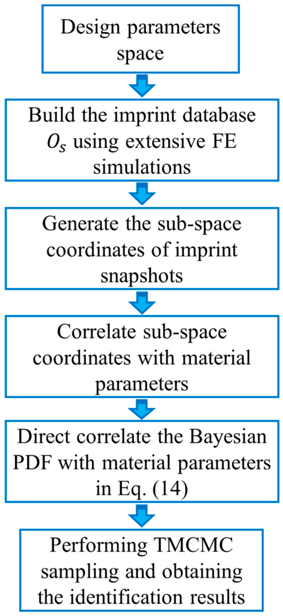
3.3. The Procedures for Identification of Elastoplastic Parameters Using the Established Measuring Method
4. Results and Discussion
4.1. The Measurement of Elastoplastic Parameters Using the Imprint Snapshot under Different Indentation Load/Depth Values
4.2. The Potential Physics Involved in the Non-Unique Posterior of Material Properties Measured by Bayesian Inference Model
4.3. Posterior Distribution of Material Parameters Obtained by Weighing the Imprint Snapshots from Different Indentation Loads
5. Conclusions
Author Contributions
Funding
Institutional Review Board Statement
Informed Consent Statement
Data Availability Statement
Conflicts of Interest
Appendix A
References
- Dao, M.; Chollacoop, N.V.; Van Vliet, K.J.; Venkatesh, T.A.; Suresh, S. Computational modeling of the forward and inverse problems in instrumented sharp indentation. Acta Mater. 2001, 49, 3899–3918. [Google Scholar] [CrossRef] [Green Version]
- Chen, X.; Ogasawara, N.; Zhao, M.; Chiba, N. On the uniqueness of measuring elastoplastic properties from indentation: The indistinguishable mystical materials. J. Mech. Phys. Solids 2007, 55, 1618–1660. [Google Scholar] [CrossRef]
- Zhang, X.; Zheng, Y.; Yang, G.; Yan, L.; Liu, L.; Cao, Y. Indentation creep tests to assess the viscoelastic properties of soft materials: Theory, method and experiment. Int. J. Non-Linear Mech. 2019, 109, 204–212. [Google Scholar] [CrossRef]
- Wang, M.; Wu, J.; Wu, H.; Zhang, Z.; Fan, H. A Novel Approach to Estimate the Plastic Anisotropy of Metallic Materials Using Cross-Sectional Indentation Applied to Extruded Magnesium Alloy AZ31B. Materials 2017, 10, 1065. [Google Scholar] [CrossRef] [PubMed] [Green Version]
- Zheng, Y.P.; Choi1, A.P.C.; Ling, H.Y.; Huang, Y.P. Simultaneous estimation of Poisson’s ratio and Young’s modulus using a single indentation: A finite element study. Meas. Sci. Technol. 2009, 20, 045706. [Google Scholar] [CrossRef]
- Wu, J.; Wang, M.; Hui, Y.; Zhang, Z.; Fan, H. Identification of anisotropic plasticity properties of materials using spherical indentation imprint mapping. Mater. Sci. Eng. A 2018, 723, 269–278. [Google Scholar] [CrossRef]
- Domínguez-Nicolas, S.M.; Herrera-May, A.L.; García-González, L.; Zamora-Peredo, L.; Hernández-Torres, J.; Martínez-Castillo, J.; Morales-González, E.A.; Cerón-Álvarez, C.A.; Escobar-Pérez, A. Algorithm for automatic detection and measurement of Vickers indentation hardness using image processing. Meas. Sci. Technol. 2021, 32, 015407. [Google Scholar] [CrossRef]
- Jeong, K.; Lee, H.; Kwon, O.M.; Jung, J.; Kwon, D.; Han, H.N. Prediction of uniaxial tensile flow using finite element-based indentation and optimized artificial neural networks. Mater. Des. 2020, 196, 109104. [Google Scholar] [CrossRef]
- Ma, Z.; Zhou, Y.; Long, S.; Zhong, X.; Lu, C. Characterization of stress-strain relationships of elastoplastic materials: An improved method with conical and pyramidal indenters. Mech. Mater. 2012, 54, 113–123. [Google Scholar] [CrossRef] [Green Version]
- Cao, Y.P.; Lu, J. Depth-sensing instrumented indentation with dual sharp indenters: Stability analysis and corresponding regularization schemes. Acta Mater. 2014, 52, 1143–1153. [Google Scholar] [CrossRef]
- Moy, C.K.; Bocciarelli, M.; Ringer, S.; Ranzi, G. Identification of the material properties of Al 2024 alloy by means of inverse analysis and indentation tests. Mater. Sci. Eng. A 2011, 529, 119–130. [Google Scholar] [CrossRef]
- Pöhl, F. Determination of unique plastic properties from sharp indentation. Int. J. Solids Struct. 2019, 171, 174–180. [Google Scholar] [CrossRef]
- Campbell, J.; Thompson, R.; Dean, J.; Clyne, T. Comparison between stress-strain plots obtained from indentation plastometry, based on residual indent profiles, and from uniaxial testing. Acta Mater. 2019, 168, 87–99. [Google Scholar] [CrossRef]
- Campbell, J.; Thompson, R.; Dean, J.; Clyne, T. Experimental and computational issues for automated extraction of plasticity parameters from spherical indentation. Mech. Mater. 2018, 124, 118–131. [Google Scholar] [CrossRef]
- Fernandez-Zelaia, P.; Joseph, V.R.; Kalidindi, S.R.; Melkote, S.N. Estimating mechanical properties from spherical indentation using Bayesian approaches. Mater. Des. 2018, 147, 92–105. [Google Scholar] [CrossRef]
- Zeng, Y.; Yu, X.; Wang, H. A new POD-based approximate bayesian computation method to identify parameters for formed AHSS. Int. J. Solids Struct. 2019, 160, 120–133. [Google Scholar] [CrossRef]
- Phadikar, J.K.; Bogetti, T.A.; Karlsson, A.M. Aspects of Experimental Errors and Data Reduction Schemes from Spherical Indentation of Isotropic Materials. J. Eng. Mater. Technol. 2014, 136, 031005. [Google Scholar] [CrossRef] [PubMed]
- Cagliero, R.; Barbato, G.; Maizza, G.; Genta, G. Measurement of elastic modulus by instrumented indentation in the macro-range: Uncertainty evaluation. Int. J. Mech. Sci. 2015, 101, 161–169. [Google Scholar] [CrossRef]
- De Bono, D.M.; London, T.; Baker, M.; Whiting, M.J. A robust inverse analysis method to estimate the local tensile properties of heterogeneous materials from nano-indentation data. Int. J. Mech. Sci. 2017, 123, 162–176. [Google Scholar] [CrossRef] [Green Version]
- Díaz, S.R. On the propagation of methodological uncertainties in Depth Sensing Indentation data analysis: A brief and critical review. Mech. Res. Commun. 2020, 105, 103516. [Google Scholar] [CrossRef]
- Benjamin, S.; Alexander, H. Determination of plastic material properties by analysis of residual imprint geometry of indentation. J. Mater. Res. 2012, 27, 2167–2177. [Google Scholar]
- Kind, N.; Berthel, B.; Fouvry, S.; Poupon, C.; Jaubert, O. Plasma-sprayed coatings: Identification of plastic properties using macro-indentation and an inverse Levenberg–Marquardt method. Mech. Mater. 2016, 98, 22–35. [Google Scholar] [CrossRef]
- Clyne, T.W.; Campbell, J.E.; Burley, M.; Dean, J. Profilometry-Based Inverse Finite Element Method Indentation Plastometry. Adv. Eng. Mater. 2021, 23, 2100437. [Google Scholar] [CrossRef]
- Shen, L.; He, Y.; Liu, D.; Gong, Q.; Zhang, B.; Lei, J. A novel method for determining surface residual stress components and their directions in spherical indentation. J. Mater. Res. 2015, 30, 1078–1089. [Google Scholar] [CrossRef]
- Bocciarelli, M.; Maier, G. Indentation and imprint mapping method for identification of residual stresses. Comput. Mater. Sci. 2007, 39, 381–392. [Google Scholar] [CrossRef]
- Tang, Y.; Campbell, J.; Burley, M.; Dean, J.; Reed, R.; Clyne, T. Profilometry-based indentation plastometry to obtain stress-strain curves from anisotropic superalloy components made by additive manufacturing. Materialia 2021, 15, 101017. [Google Scholar] [CrossRef]
- Oviasuyi, R.; Klassen, R. Deducing the stress–strain response of anisotropic Zr–2.5%Nb pressure tubing by spherical indentation testing. J. Nucl. Mater. 2013, 432, 28–34. [Google Scholar] [CrossRef]
- Yu, H.; Das, S.; Yu, H.; Karamched, P.; Tarleton, E.; Hofmann, F. Orientation dependence of the nano-indentation behaviour of pure Tungsten. Scr. Mater. 2020, 189, 135–139. [Google Scholar] [CrossRef]
- Han, Q.-N.; Rui, S.-S.; Qiu, W.; Su, Y.; Ma, X.; Su, Z.; Cui, H.; Shi, H. Effect of crystal orientation on the indentation behaviour of Ni-based single crystal superalloy. Mater. Sci. Eng. A 2020, 773, 138893. [Google Scholar] [CrossRef]
- Renner, E.; Bourceret, A.; Gaillard, Y.; Amiot, F.; Delobelle, P.; Richard, F. Identifiability of single crystal plasticity parameters from residual topographies in Berkovich nanoindentation on FCC nickel. J. Mech. Phys. Solids 2020, 138, 103916. [Google Scholar] [CrossRef]
- Honarmandi, P.; Arroyave, R. Using Bayesian framework to calibrate a physically based model describing strain-stress behavior of TRIP steels. Comput. Mater. Sci. 2017, 129, 66–81. [Google Scholar] [CrossRef] [Green Version]
- Ortiz, G.A.; Alvarez, D.A.; Bedoya-Ruíz, D. Identification of Bouc–Wen type models using the Transitional Markov Chain Monte Carlo method. Comput. Struct. 2015, 146, 252–269. [Google Scholar] [CrossRef]
- Madireddy, S.; Sista, B.; Vemaganti, K. A Bayesian approach to selecting hyperelastic constitutive models of soft tissue. Comput. Methods Appl. Mech. Eng. 2015, 291, 102–122. [Google Scholar] [CrossRef]
- Zhang, C.; Liu, M.; Meng, Z.; Zhang, Q.; Zhao, G.; Chen, L.; Zhang, H.; Wang, J. Microstructure evolution and precipitation characteristics of spray-formed and subsequently extruded 2195 Al-Li alloy plate during solution and aging process. J. Mater. Process. Technol. 2020, 283, 116718. [Google Scholar] [CrossRef]
- Chen, X.; Lei, Z.; Chen, Y.; Han, B.; Jiang, M.; Tian, Z.; Bi, J.; Lin, S. Nano-indentation and in-situ investigations of double-sided laser beam welded 2060-T8/2099-T83 Al-Li alloys T-joints. Mater. Sci. Eng. A 2019, 756, 291–301. [Google Scholar] [CrossRef]
- Buljak, V.; Maier, G. Proper Orthogonal Decomposition and Radial Basis Functions in material characterization based on instrumented indentation. Eng. Struct. 2011, 33, 492–501. [Google Scholar] [CrossRef]
- Liang, Y.; Lee, H.; Lim, S.; Lin, W.; Lee, K.; Wu, C. Proper orthogonal decomposition and its applications—part I: Theory. J. Sound Vib. 2002, 252, 527–544. [Google Scholar] [CrossRef]
- Ghnatios, C.; Mathis, C.; Chinesta, F. Poroelastic properties identification through micro indentation modeled by using the proper generalized decomposition. In Proceedings of the 2016 3rd International Conference on Advances in Computational Tools for Engineering Applications (ACTEA), Zouk-Mosbeh, Lebanon, 13–15 July 2016; pp. 141–145. [Google Scholar]
- Ching, J.; Chen, Y.-C. Transitional Markov Chain Monte Carlo Method for Bayesian Model Updating, Model Class Selection, and Model Averaging. J. Eng. Mech. 2007, 133, 816–832. [Google Scholar] [CrossRef]
- ABAQUS. Analysis User’s Manual v 6.9; ABAQUS Inc.: Providence, RI, USA, 2009. [Google Scholar]
- Moharrami, R.; Sanayei, M. Numerical study of the effect of yield strain and stress ratio on the measurement accuracy of biaxial residual stress in steels using indentation. J. Mater. Res. Technol. 2020, 9, 3950–3957. [Google Scholar] [CrossRef]
- Bowden, F.P.; Tabor, D. The Friction and Lubrication of Solids; Oxford University Press: Oxford, UK, 2001. [Google Scholar]
- Pöhl, F.; Huth, S.; Theisen, W. Indentation of self-similar indenters: An FEM-assisted energy-based analysis. J. Mech. Phys. Solids 2014, 66, 32–41. [Google Scholar] [CrossRef]


| Material | E (GPa) | n | |
|---|---|---|---|
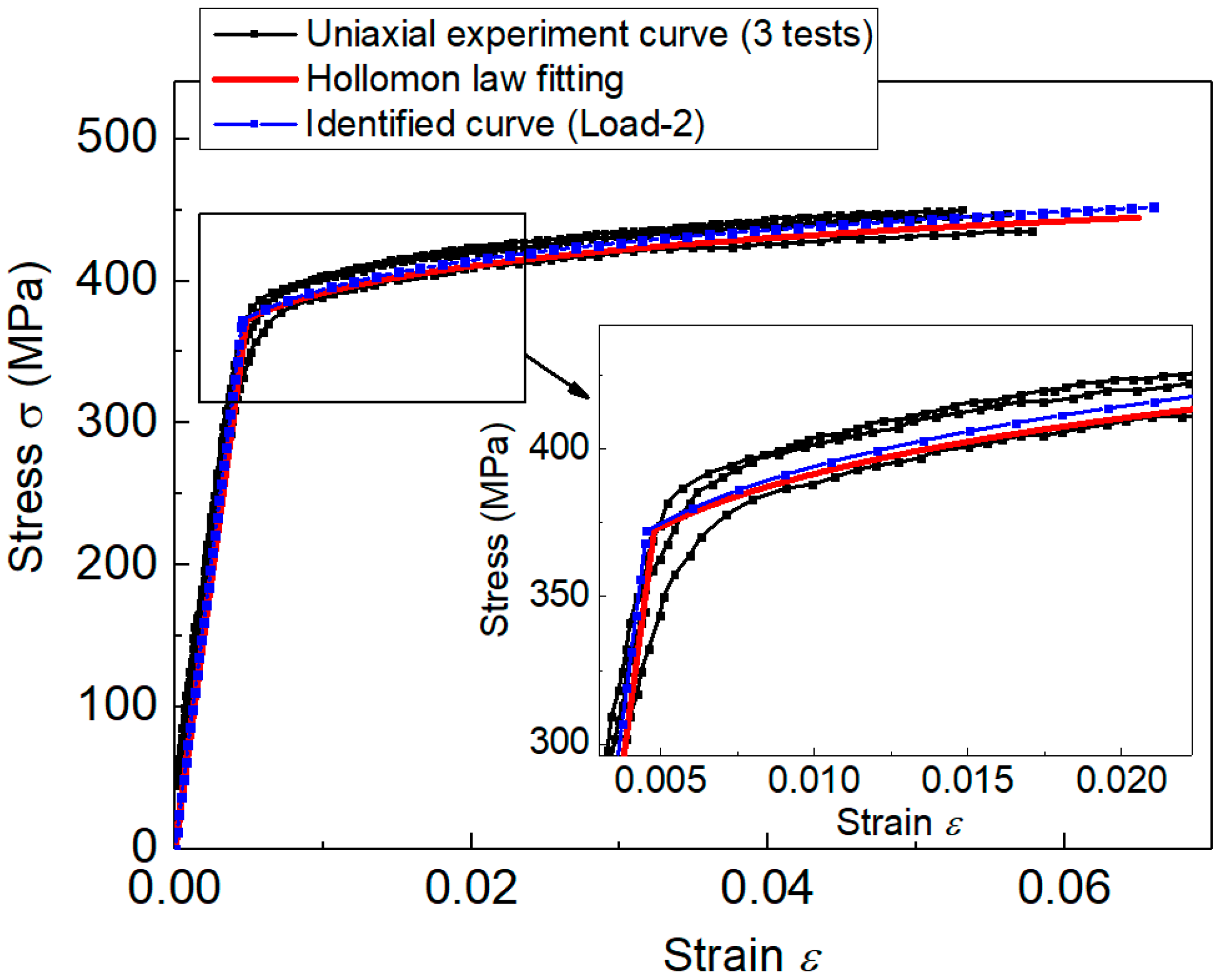
| Al-Li alloys | 77.7 | 372.6 | 0.0678 |
| Al-Li Alloys | |||
|---|---|---|---|
| Uniaxial properties | 77.6 | 372.6 | 0.0678 |
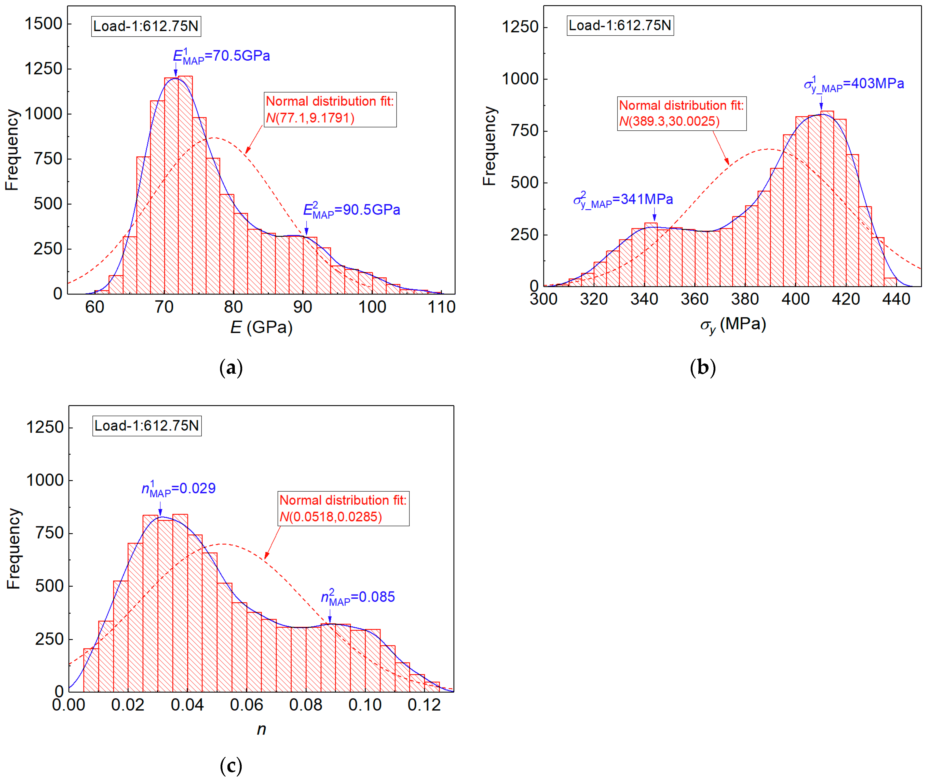
| Indentation: (Load-1) | |||
| MAP value 1 | 70.5 | 403.0 | 0.029 |
| Error (%) | −9.15 | 8.16 | −57.23 |
| MAP value 2 | 90.5 | 341.0 | 0.085 |
| Error (%) | 16.62 | −8.48 | 25.37 |
| MEAN value | 77.1 | 389.3 | 0.0518 |
| Error (%) | −0.64 | 4.48 | −23.60 |
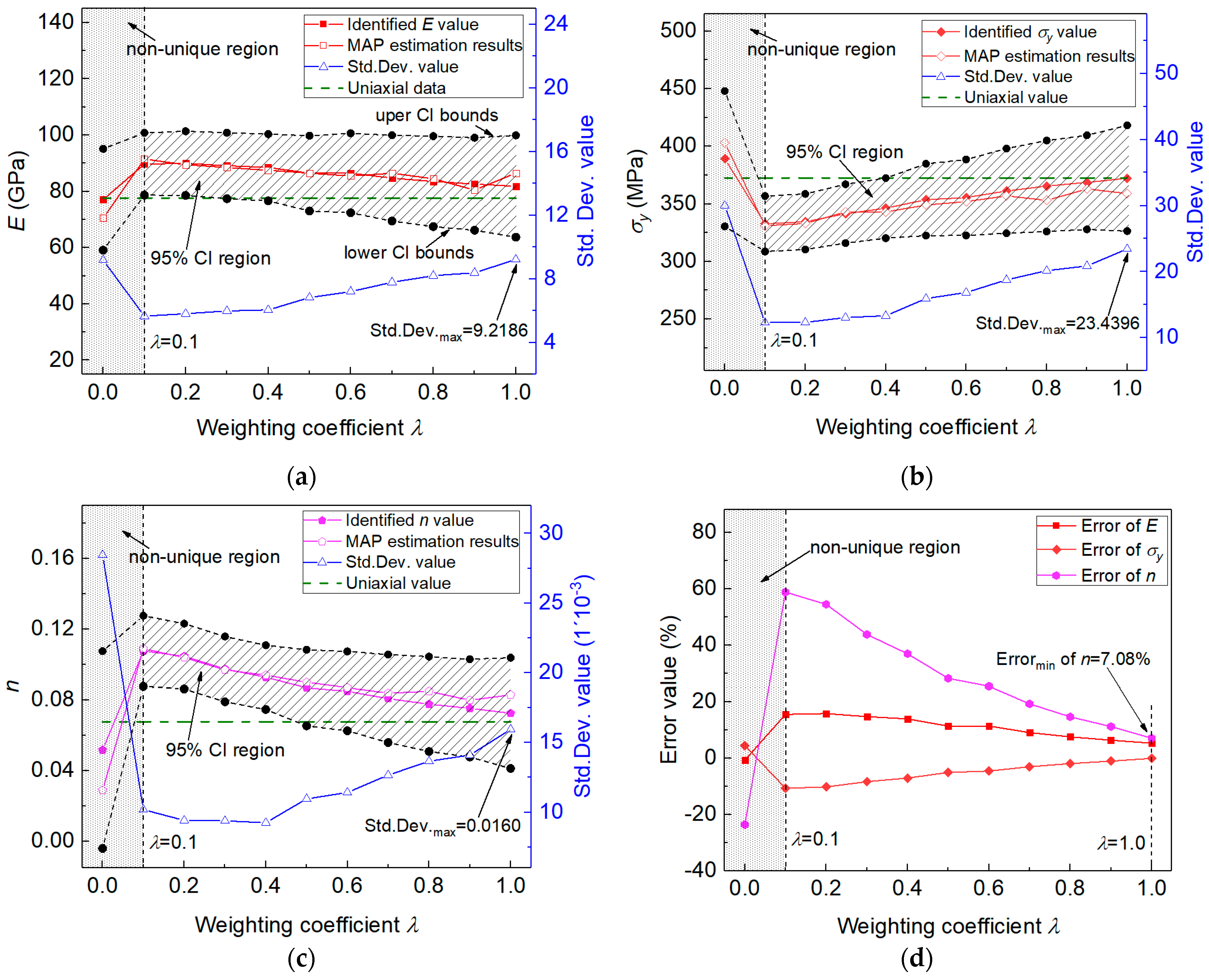
| Std. Dev. | 9.18 | 30.00 | 0.0285 |
| Al-Li Alloys | |||
|---|---|---|---|
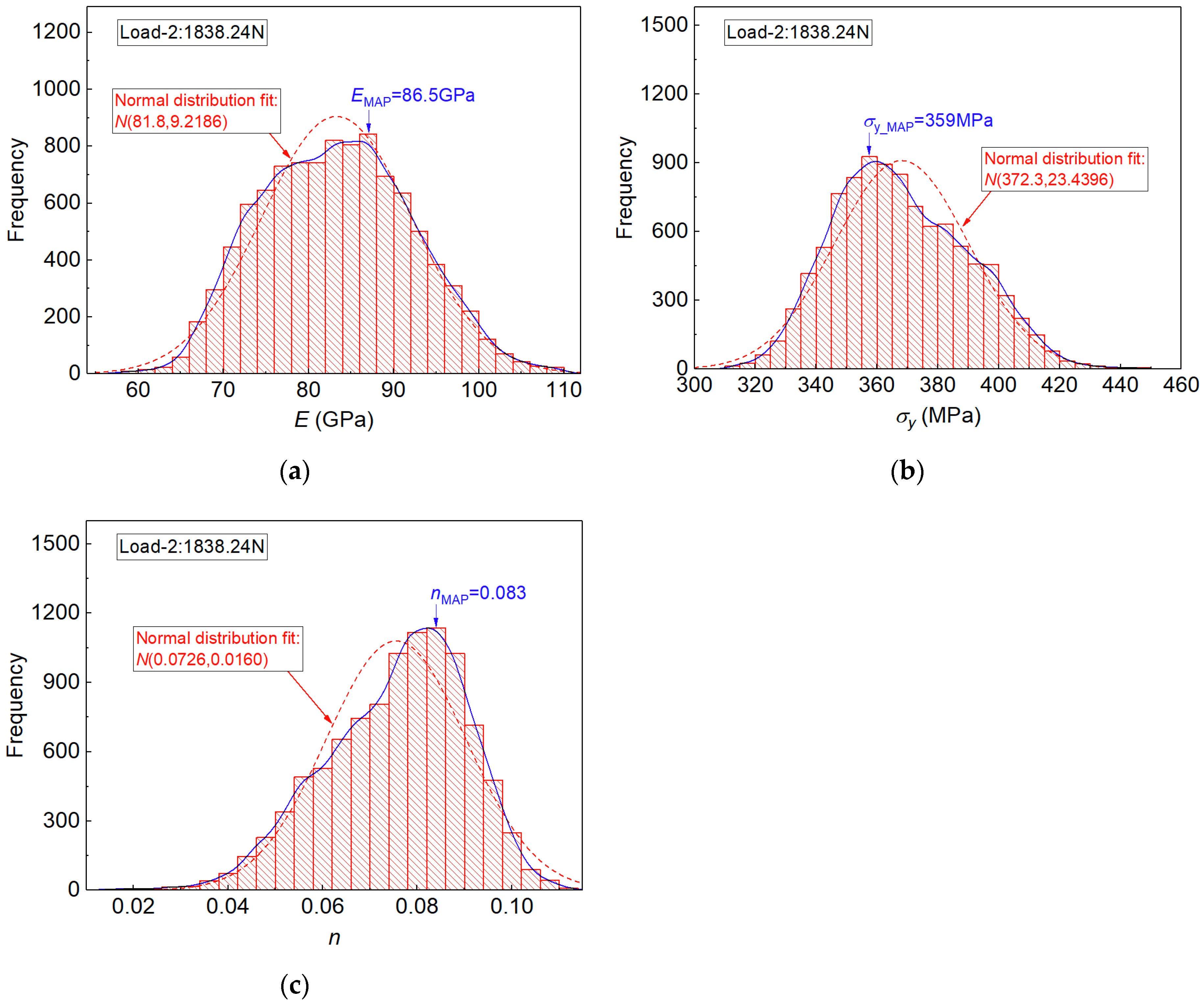
| Uniaxial properties | 77.6 | 372.6 | 0.0678 |
| Indentation (Load-2) | |||
| MAP value | 86.5 | 359 | 0.083 |
| Error (%) | 11.47 | −3.65 | 22.42 |
| MEAN value | 81.8 | 372.3 | 0.0726 |
| Std. Dev. | 9.2186 | 23.4396 | 0.01595 |
| Error (%) | 5.41 | −0.081 | 7.08 |
Publisher’s Note: MDPI stays neutral with regard to jurisdictional claims in published maps and institutional affiliations. |
© 2021 by the authors. Licensee MDPI, Basel, Switzerland. This article is an open access article distributed under the terms and conditions of the Creative Commons Attribution (CC BY) license (https://creativecommons.org/licenses/by/4.0/).
Share and Cite
Wang, M.; Wang, W. An Inverse Method for Measuring Elastoplastic Properties of Metallic Materials Using Bayesian Model and Residual Imprint from Spherical Indentation. Materials 2021, 14, 7105. https://doi.org/10.3390/ma14237105
Wang M, Wang W. An Inverse Method for Measuring Elastoplastic Properties of Metallic Materials Using Bayesian Model and Residual Imprint from Spherical Indentation. Materials. 2021; 14(23):7105. https://doi.org/10.3390/ma14237105
Chicago/Turabian StyleWang, Mingzhi, and Weidong Wang. 2021. "An Inverse Method for Measuring Elastoplastic Properties of Metallic Materials Using Bayesian Model and Residual Imprint from Spherical Indentation" Materials 14, no. 23: 7105. https://doi.org/10.3390/ma14237105
APA StyleWang, M., & Wang, W. (2021). An Inverse Method for Measuring Elastoplastic Properties of Metallic Materials Using Bayesian Model and Residual Imprint from Spherical Indentation. Materials, 14(23), 7105. https://doi.org/10.3390/ma14237105