
Particle Size Measurement Using Dynamic Light Scattering at Ultra-Low Concentration Accounting for Particle Number Fluctuations

 ,
,
Abstract
:1. Introduction
2. Theory and Methods
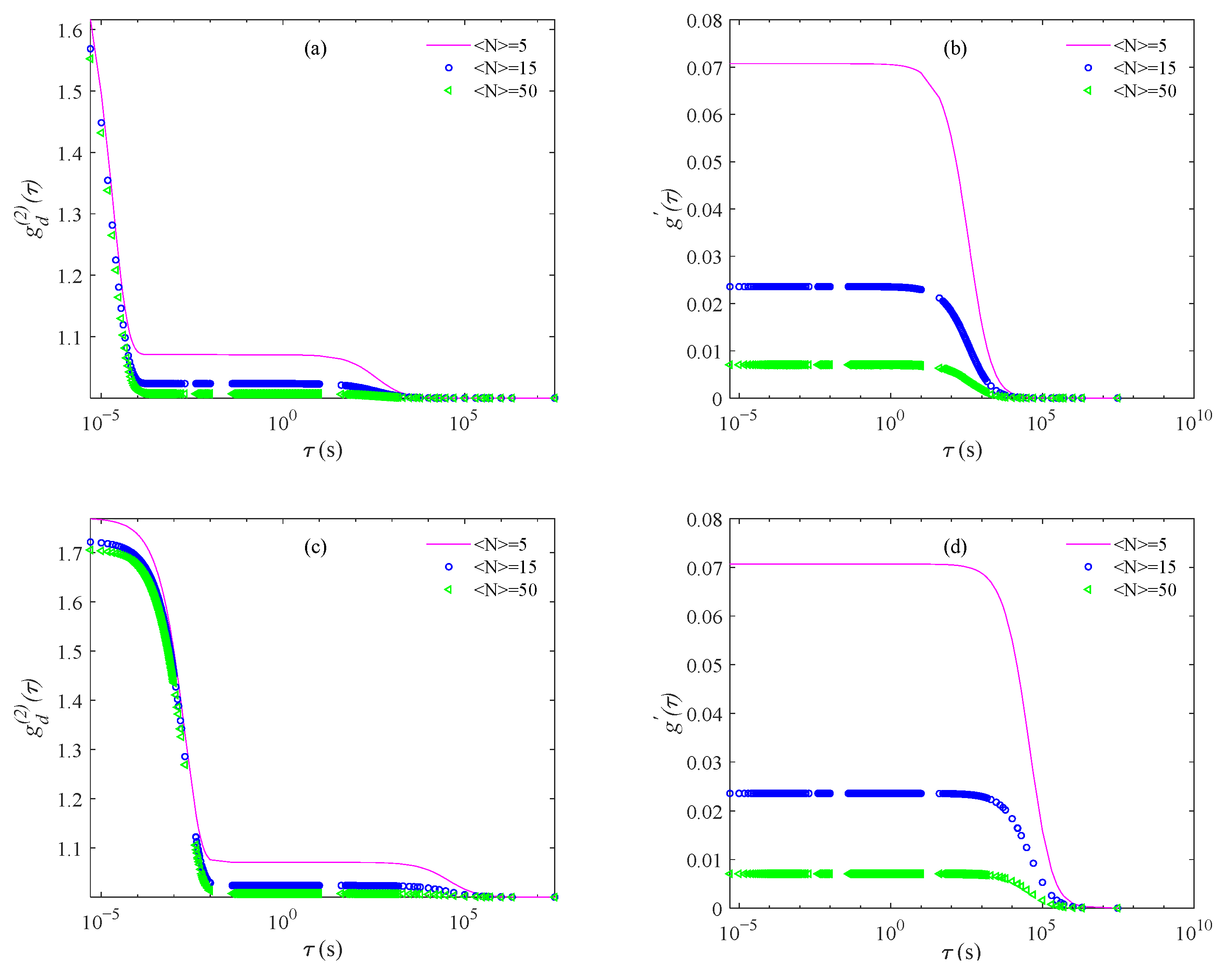
2.1. Classical DLS Theory and Number Fluctuations in the Scattering Volume
2.2. PSD Recovery from DLS Measurements at Ultra-Low Concentrations
2.2.1. Kernel Function Reconstruction of Inversion Equation
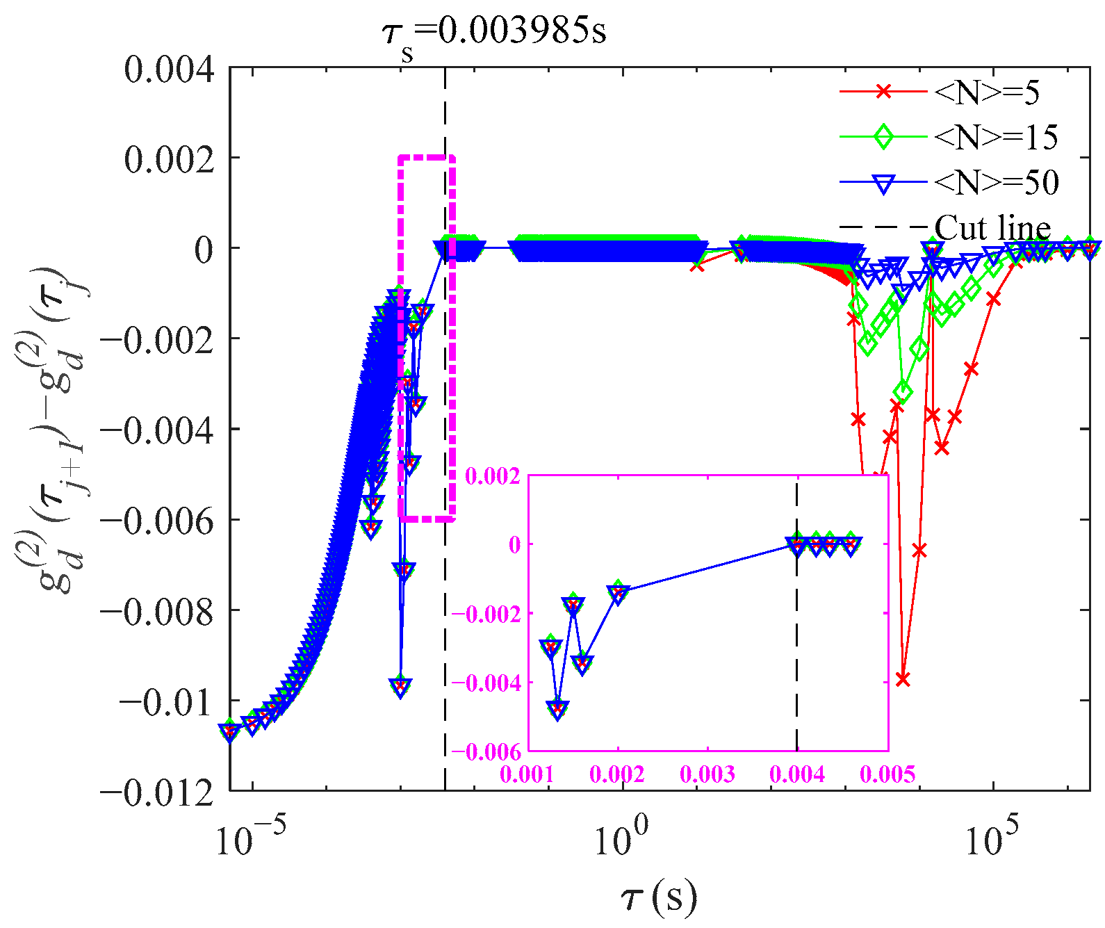
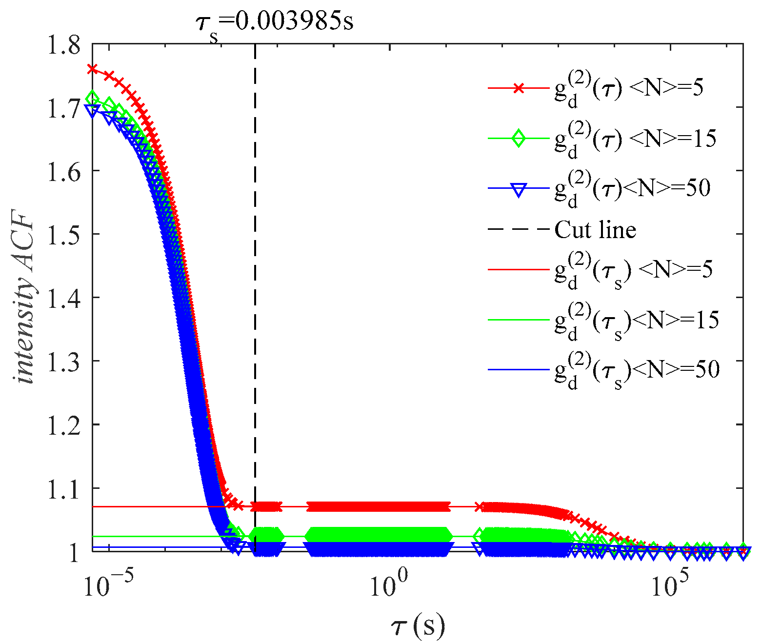
2.2.2. Intensity ACF Baseline Reset
3. Results
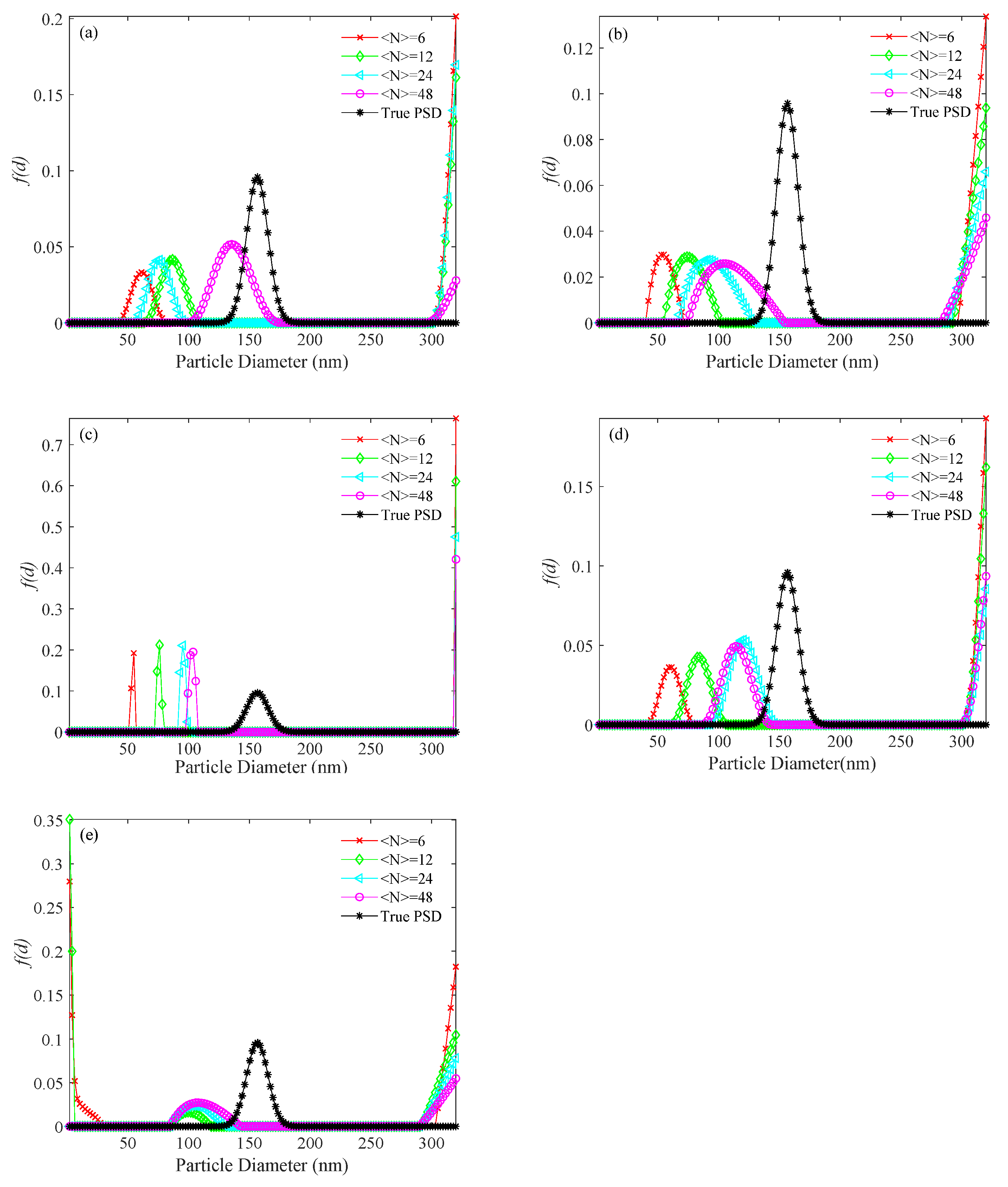
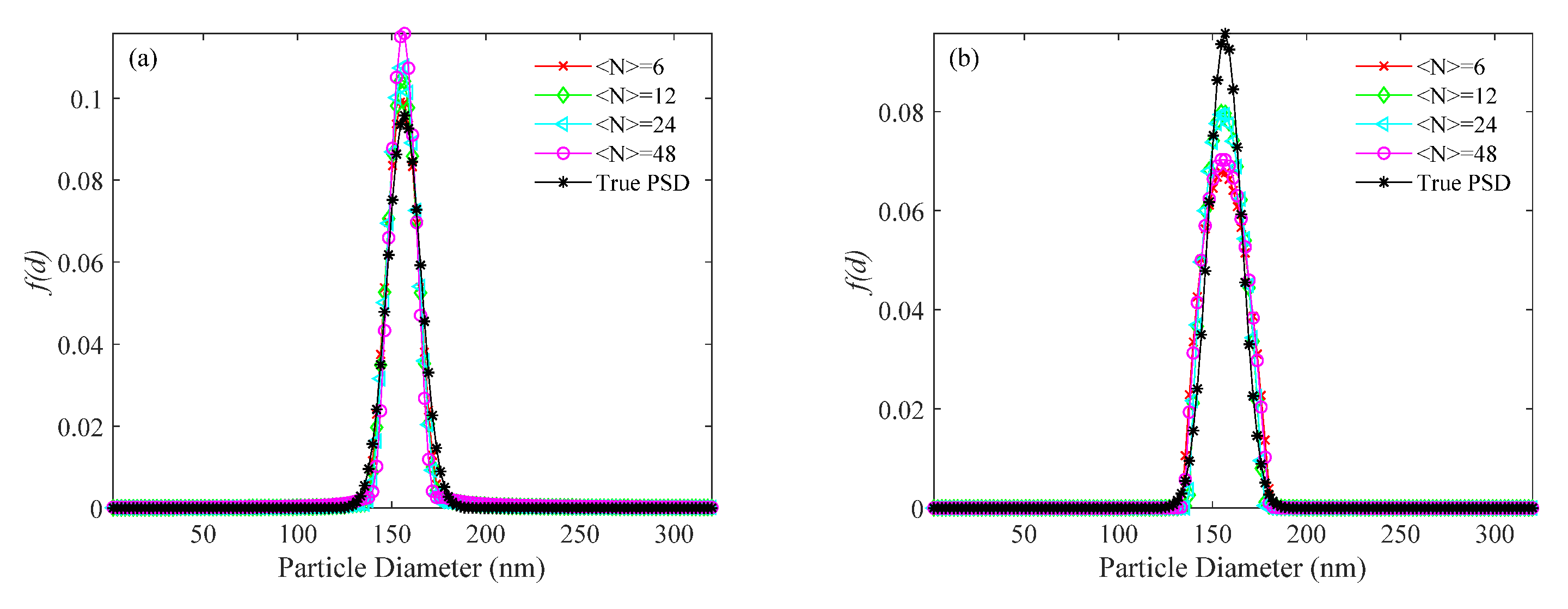
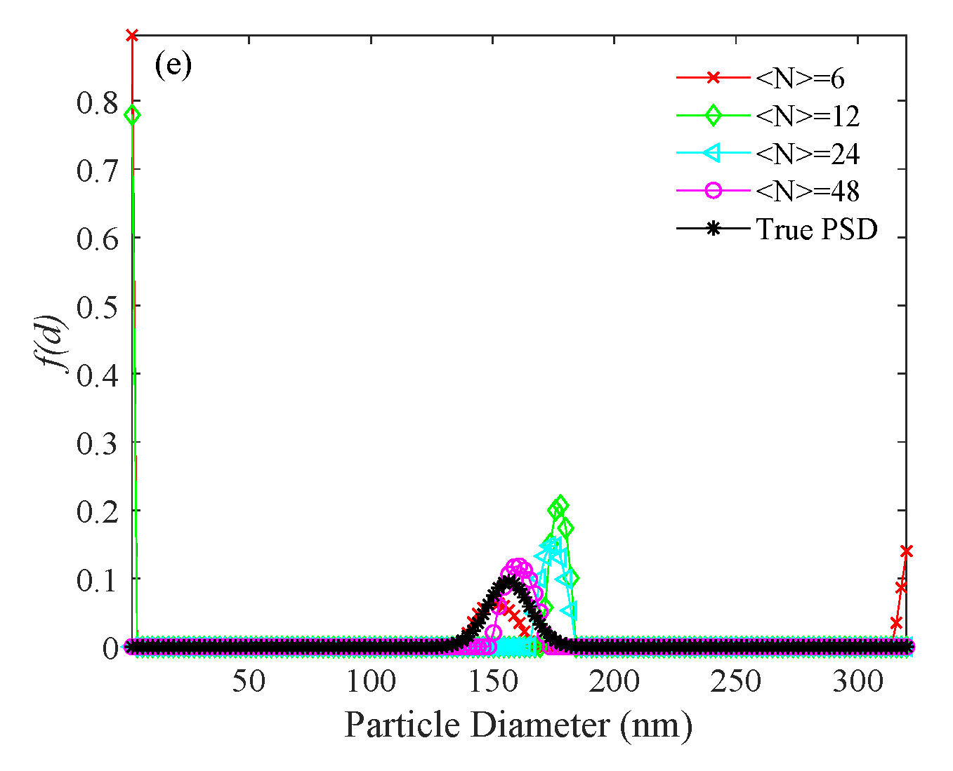
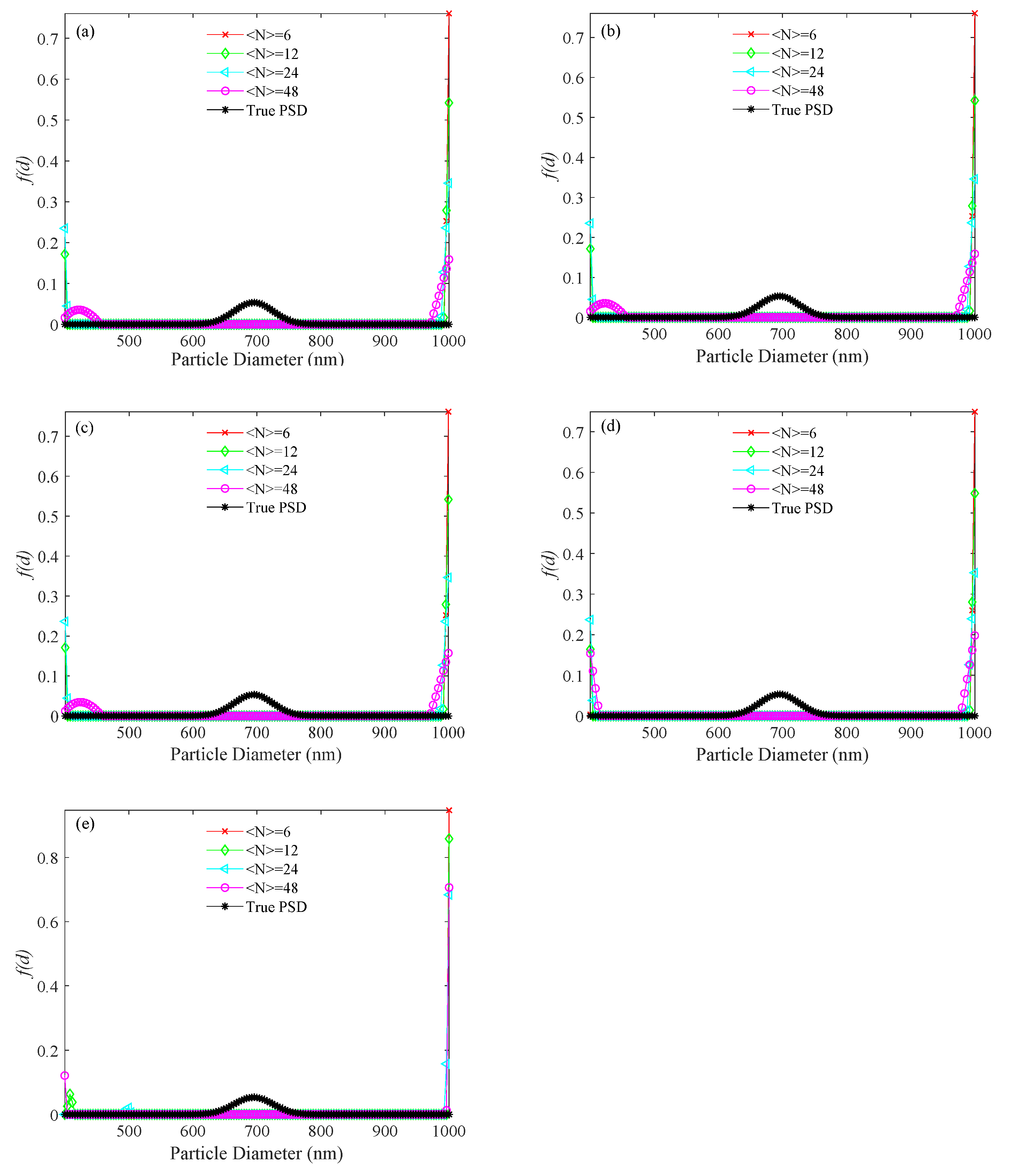
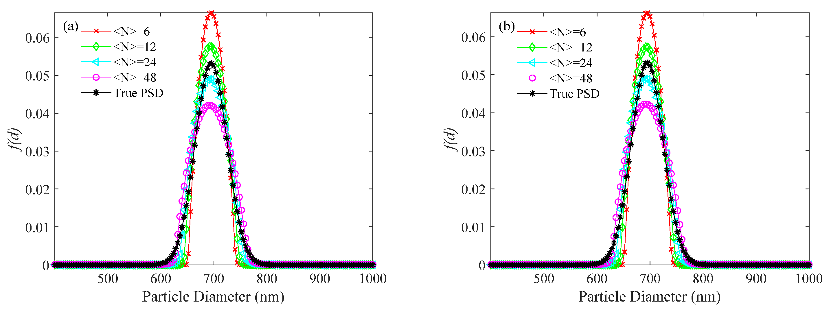
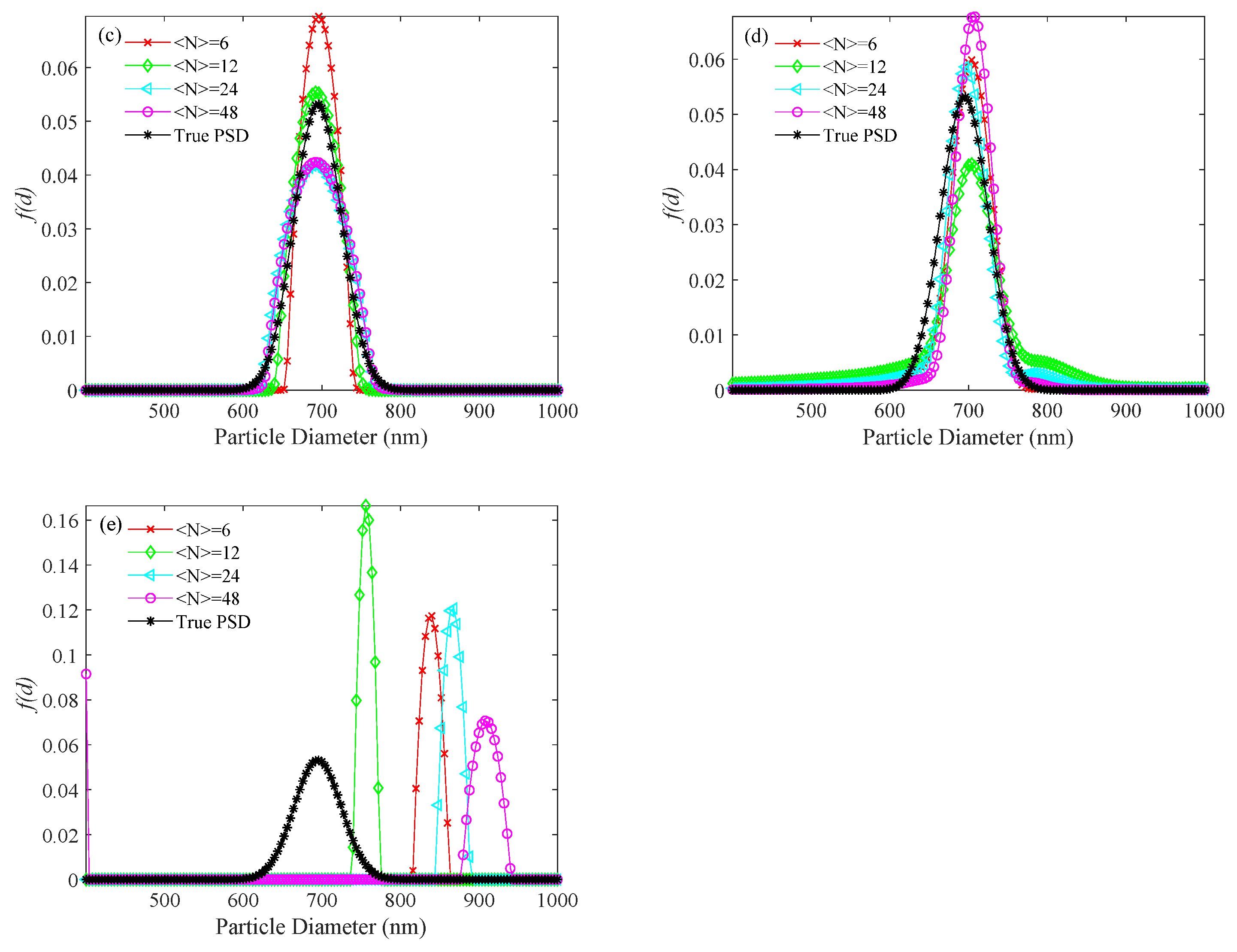
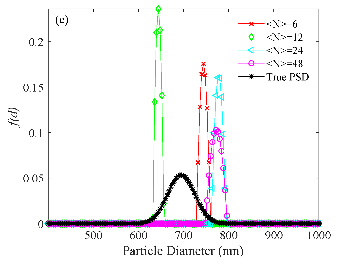
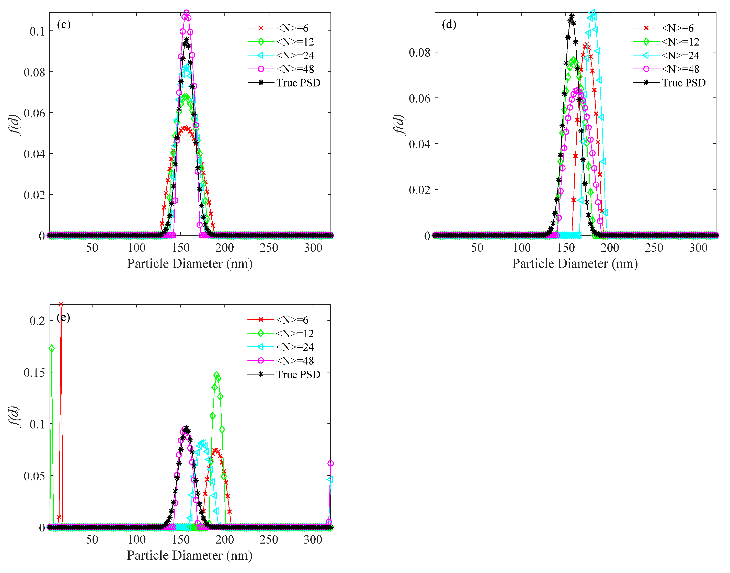
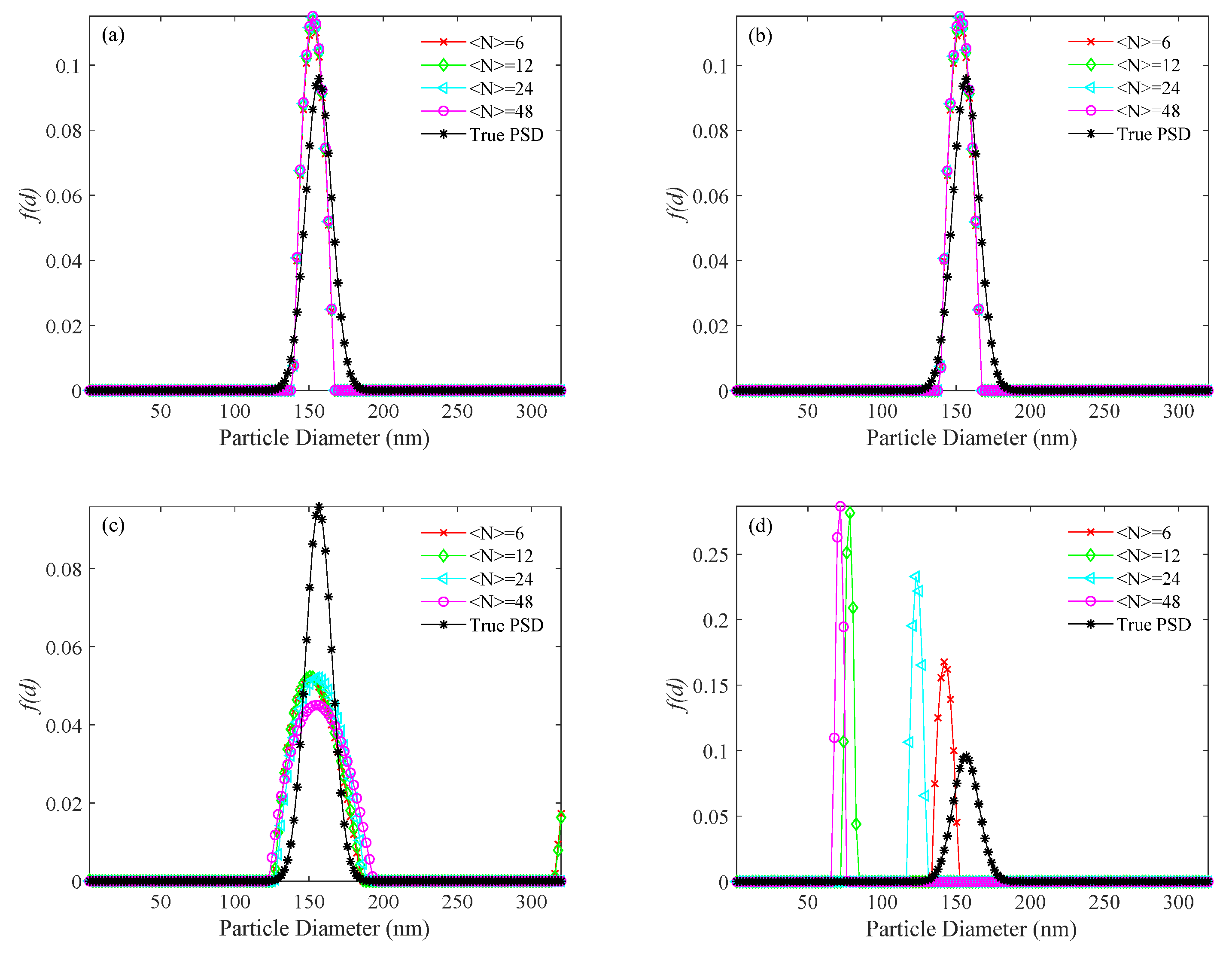
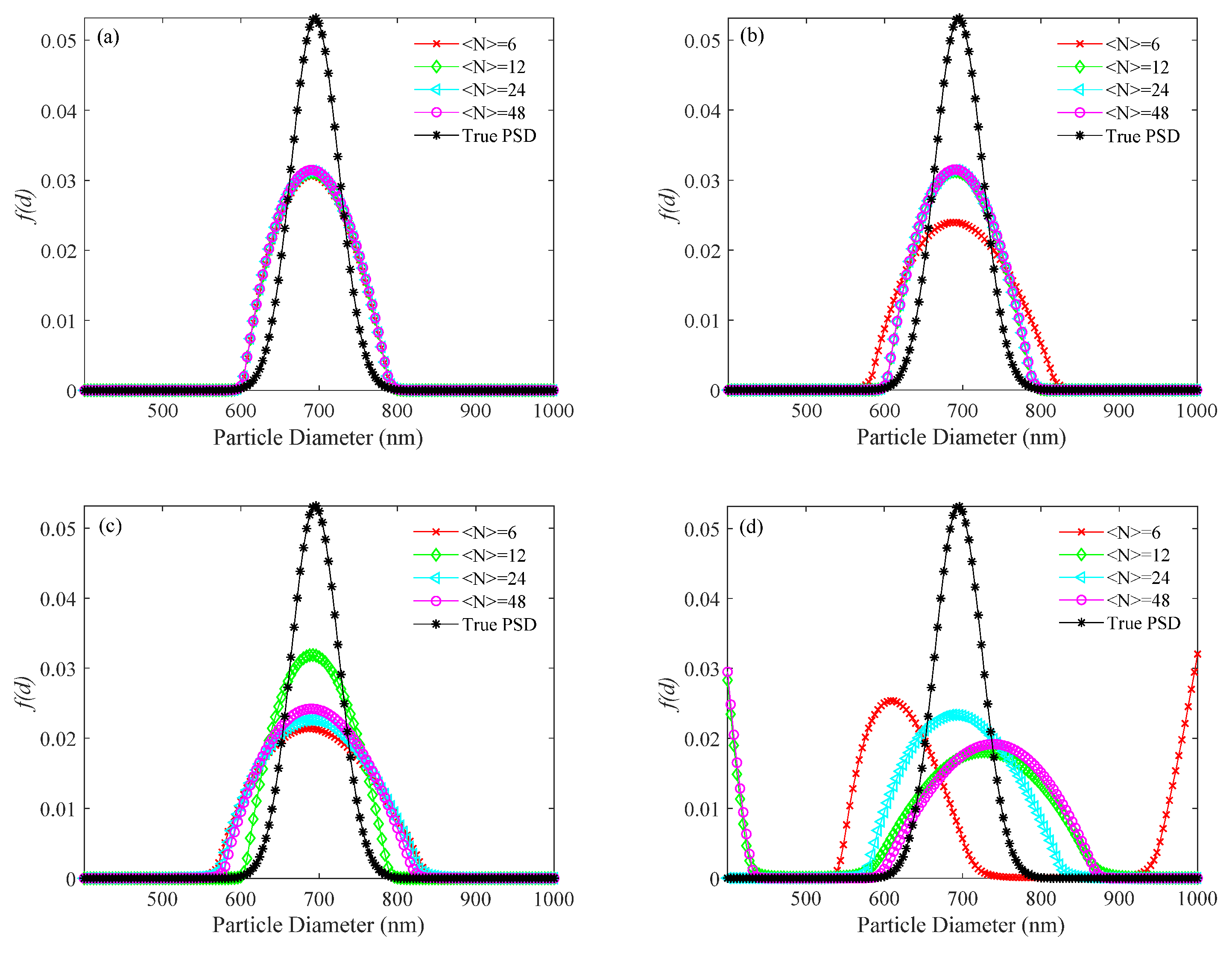
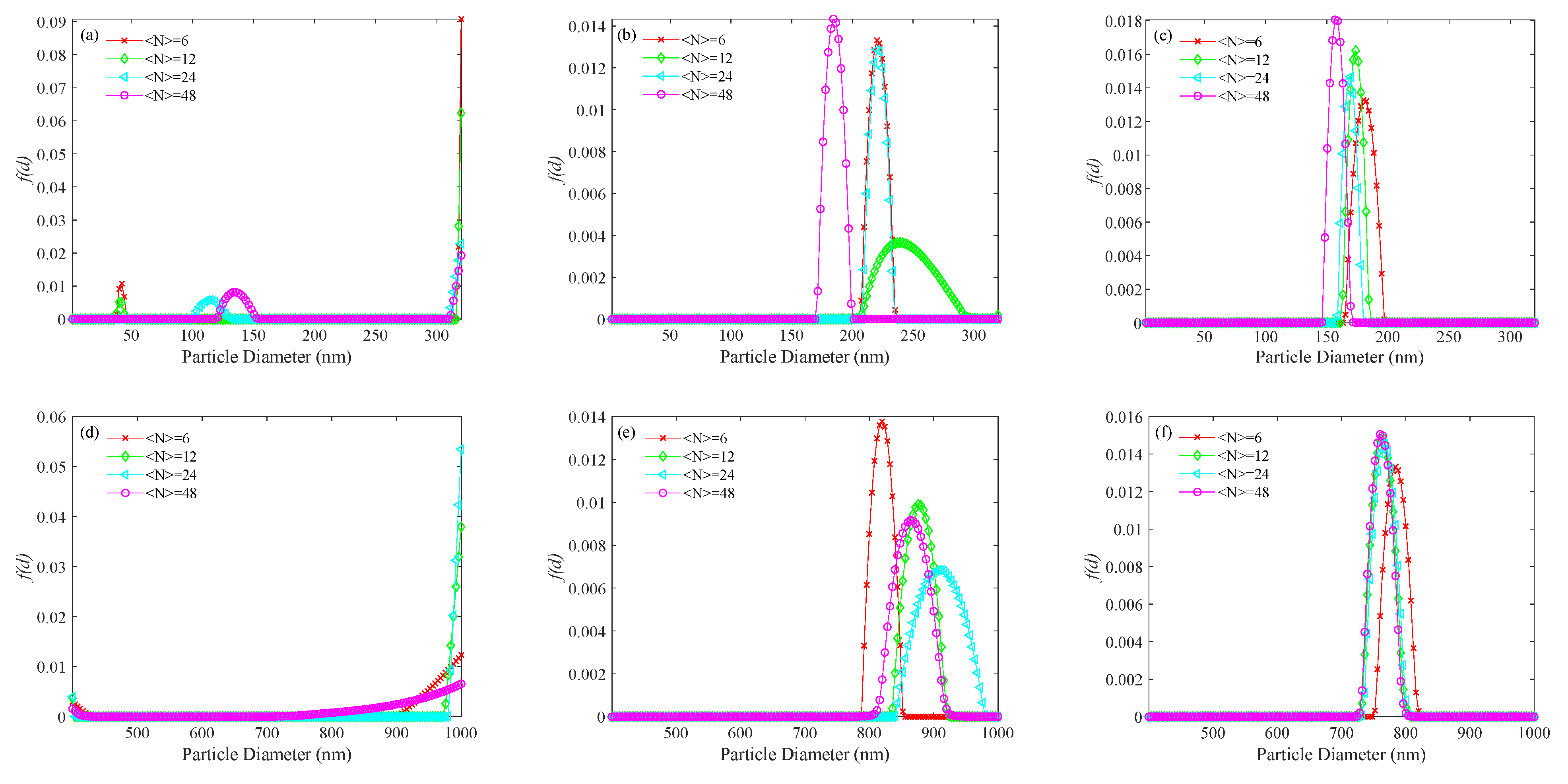
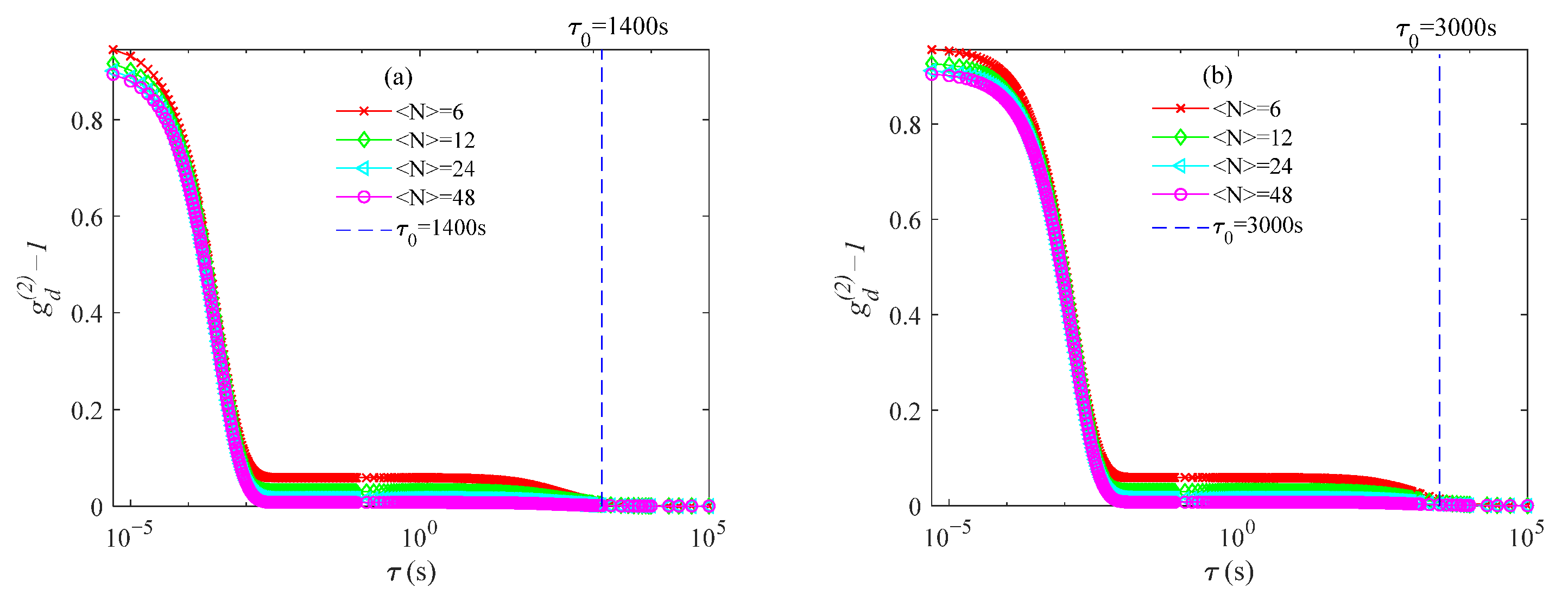
3.1. Simulation
3.2. Experiment
4. Discussion
5. Conclusions
Author Contributions
Funding
Institutional Review Board Statement
Informed Consent Statement
Data Availability Statement
Conflicts of Interest
References
- Pecora, R. Doppler shifts in light scattering from pure liquids and polymer solutions. J. Chem. Phys. 1964, 40, 1604–1614. [Google Scholar] [CrossRef]
- Cummins, H.Z.; Knable, N.; Yeh, Y. Observation of diffusion broadening of raleigh scattered light. Phys. Rev. Lett. 1964, 12, 150–153. [Google Scholar] [CrossRef]
- Ford, N.C.; Benedek, G.B. Observation of the spectrum of light scattered from a pure fluid near its critical point. Phys. Rev. Lett. 1965, 15, 649–653. [Google Scholar] [CrossRef]
- Pike, E.R. The Malvern correlator. Case study in development. Phys. Technol. 1979, 10, 104–109. [Google Scholar] [CrossRef]
- Pike, E.R. Lasers, photon statistics, photon-correlation spectroscopy and subsequent applications. J. Eur. Opt. Soc. Rapid 2010, 5, 138. [Google Scholar] [CrossRef]
- Gómez-Merino, A.I.; Rubio-Hernández, F.J.; Velázquez-Navarro, J.F.; Aguiar, J.; Jiménez-Agredano, C. Study of the aggregation state of anatase water nanofluids using rheological and DLS methods. Ceram. Int. 2014, 40, 14045–14050. [Google Scholar] [CrossRef]
- Hou, J.; Ci, H.; Wang, P.; Wang, C.; Lv, B.; Miao, L.; You, G. Nanoparticle tracking analysis versus dynamic light scattering: Case study on the effect of Ca2+ and alginate on the aggregation of cerium oxide nanoparticles. J. Hazard. Mater. 2018, 360, 319–328. [Google Scholar] [CrossRef]
- Zhan, S.; Hu, J.; Li, Y.; Huang, X.; Xiong, Y. Direct competitive ELISA enhanced by dynamic light scattering for the ultrasensitive detection of aflatoxin B1 in corn samples. Food Chem. 2021, 342, 128327. [Google Scholar] [CrossRef] [PubMed]
- Carvalho, J.W.P.; Santiago, P.S.; Batista, T.; Salmon, C.E.G.; Barbosa, L.R.S.; Itri, R.; Tabak, M. On the temperature stability of extracellular hemoglobin of Glossoscolex paulistus, at different oxidation states: SAXS and DLS studies. Biophys. Chem. 2012, 163–164, 44–55. [Google Scholar] [CrossRef]
- Bai, M.; Bai, C.; Daisuke, A.; Hiromu, T.; Kensuke, M.; Takashi, Y. Role of a long-chain alkyl group in sulfated alkyl oligosaccharides with high anti-HIV activity revealed by SPR and DLS. Carbohyd. Polym. 2020, 245, 116518. [Google Scholar] [CrossRef]
- Pecora, R. Dynamic Light Scattering Measurement of Nanometer Particles in Liquids. J. Nanopart. Res. 2000, 2, 123–131. [Google Scholar] [CrossRef]
- International Organization for Standardization. Particle Size Analysis–Photon Correlation Spectroscopy: ISO 13321[S]; International Organization for Standardization: Geneva, Switzerland, 1996. [Google Scholar]
- International Organization for Standardization. Particle Size Analysis–Dynamic Light Scattering (DLS): ISO 22412:2008[S]; International Organization for Standardization: Geneva, Switzerland, 2008. [Google Scholar]
- International Organization for Standardization. Particle Size Analysis–Dynamic Light Scattering (DLS): ISO 22412:2017[S]; International Organization for Standardization: Geneva, Switzerland, 2017. [Google Scholar]
- Thomas, J.C. Photon correlation spectroscopy: Technique and instrumentation. Proc. SPIE 1991, 1430, 2–18. [Google Scholar] [CrossRef]
- Bunkin, N.F.; Shkirin, A.V.; Chirikov, S.N.; Sendrovitz, A.L. Effect of the spatial distribution of probe beam on the results of measurements of the disperse composition of nanoparticles by dynamic light scattering method. Bull. Lebedev Phys. Inst. 2016, 43, 252–255. [Google Scholar] [CrossRef]
- Kirichenko, M.N.; Sanoeva, A.T.; Chaikov, L.L. Appearance of an Artifact Peak in the Particle Size Distribution Measured by DLS at Low Concentrations. Bull. Lebedev Phys. Inst. 2016, 43, 256–260. [Google Scholar] [CrossRef]
- Bunkin, N.F.; Shkirin, A.V.; Suyazov, N.V.; Chaikov, L.L.; Chirikov, S.N.; Kirichenko, M.N.; Nikiforov, S.D.; Tymper, S.I. Influence of low concentrations of scatterers and signal detection time on the results of their measurements using dynamic light scattering. Quantum Electron. 2017, 47, 949–955. [Google Scholar] [CrossRef]
- Yang, H.; Yang, H.; Kong, P.; Zhu, Y.; Dai, S.; Zheng, G. Concentration measurement of particles by number fluctuation in dynamic light backscattering. Powder Technol. 2013, 246, 499–503. [Google Scholar] [CrossRef]
- Willemse, A.W.; Drunen, M.A.V.; Tuinman, I.L.; Marijnisse, J.C.M.; Merkus, H.G.; Scarlett, B. Photon correlation spectroscopy for analysis of low concentration aerosols. J. Aerosol Sci. 1995, 26, S31–S32. [Google Scholar] [CrossRef]
- Wuyckhuyse, A.L.V.; Willemse, A.W.; Marijnissen, J.C.M.; Scarlett, B. Determination of on-line particle size and concentration for sub-micron particles at low concentrations. J. Aerosol Sci. 1996, 27, S577–S578. [Google Scholar] [CrossRef]
- Willemse, A.W.; Marijnissen, J.C.M.; Roos, R.; Wuyckhuyse, A.L.V.; Scarlett, B. Photon correlation spectroscopy for analysis of low concentration submicrometer samples. J. Aerosol Sci. 1996, 27, S535–S536. [Google Scholar] [CrossRef]
- Willemse, A.W.; Marijnissen, J.C.M.; Wuyckhuyse, A.L.V.; Roos, R.; Merkus, H.G.; Scarlett, B. Low-concentration photon correlation spectroscopy. Part. Part. Syst. Charact. 1997, 14, 157–162. [Google Scholar] [CrossRef]
- Willemse, A.W.; Marijnissen, J.C.M.; Wuyckhuyse, A.L.V.; Roos, R.; Merkus, H.G.; Scarlett, B. Photon correlation spectroscopy for analysis of low concentration submicrometer samples. Progr. Colloid Polym. Sci. 1997, 104, 113–116. [Google Scholar] [CrossRef]
- Schaefer, D.W.; Berne, B.J. Light scattering from Non-Gaussian concentration fluctuations. Phys. Rev. Lett. 1972, 28, 475–478. [Google Scholar] [CrossRef]
- Chaikov, L.; Kirichenko, M.N.; Krivokhizha, S.V.; Zaritskiy, A.R. Dynamics of statistically confident particle sizes and concentrations in blood plasma obtained by the dynamic light scattering method. J. Biomed. Opt. 2015, 20, 57003. [Google Scholar] [CrossRef] [PubMed]
- Kirichenko, M.N.; Masalov, A.V.; Chaikov, L.L.; Zaritskii, A.R. Relation between particle sizes and concentration in undiluted and diluted blood plasma according to light scattering data. Bull. Lebedev Phys. Inst. 2015, 42, 33–36. [Google Scholar] [CrossRef]
- Surianarayanan, R.; Shivakumar, H.G.; Vegesna, N.S.K.V.; Srivastava, A. Effect of sample Concentration on the Characterization of Liposomes using Dynamic light Scattering Technique. Pharm. Methods 2016, 7, 70–74. [Google Scholar] [CrossRef] [Green Version]
- Schatzel, K. Correlation techniques in dynamic light scattering. Appl. Phys. B 1987, 42, 193–213. [Google Scholar] [CrossRef]
- Nijman, E.J.; Merkus, H.G.; Marijnissen, J.C.M.; Scarlett, B. Simulations and experiments on number fluctuations in photon-correlation spectroscopy at low particle concentrations. Appl. Opt. 2001, 40, 4058–4063. [Google Scholar] [CrossRef]
- Yu, A.B.; Standish, N. A study of particle size distribution. Powder Technol. 1990, 62, 101–118. [Google Scholar] [CrossRef]
- Xu, M.; Shen, J.; Thomas, J.C.; Huang, Y.; Zhu, X.; Clementi, L.A.; Vega, J.R. Information-weighted constrained regularization for particle size distribution recovery in multiangle dynamic light scattering. Opt. Express 2018, 26, 15–31. [Google Scholar] [CrossRef]
- Xu, M.; Shen, J.; Huang, Y.; Xu, Y.; Zhu, X.; Wang, Y.; Liu, W.; Gao, M. Weighting inversion of dynamic light scattering based on particle-size information distribution character. Acta Phys. Sin. 2018, 67, 134201. [Google Scholar] [CrossRef]
- Nijman, E.J.; Merkus, H.G.; Marijnissen, J.C.M.; Scarlett, B. Investigation of the influence of low particle concentration on photon correlation spectroscopy. In Photon. Correlation and Scattering; Optical Society of America: Whistler, BC, Canada, 2000. [Google Scholar] [CrossRef]


| Particle Size (nm) | <N> | Δg′ | tc (s) | td (s) |
|---|---|---|---|---|
| 10 | 5 | 1.0 × 10⁻⁸ | 3.0 × 10⁻⁵ | 1.0 × 10⁻⁴ |
| 15 | 3.3 × 10⁻⁹ | 3.0 × 10⁻⁵ | 5.0 × 10⁻³ | |
| 50 | 1.0 × 10⁻⁹ | 3.0 × 10⁻⁵ | 2.0 × 10⁻³ | |
| 1000 | 5 | 1.6 × 10⁻⁸ | 4.0 × 10⁻³ | 1.0 × 10⁻⁶ |
| 15 | 5.2 × 10⁻⁹ | 4.0 × 10⁻³ | 4.0 × 10⁻⁵ | |
| 50 | 1.6 × 10⁻⁹ | 4.0 × 10⁻³ | 2.0 × 10⁻⁵ |
| P (nm) | μ | σ | (dmin, dmax) (nm) |
|---|---|---|---|
| 156 | 0.50 | 9.0 | (2, 320) |
| 696 | 0.17 | 5.0 | (400, 1000) |
| δ | <N> | PU (nm) | PKFR (nm) | PBR (nm) | EPU | EPKFR | EPBR | VEU | VEKFR | VEBR |
|---|---|---|---|---|---|---|---|---|---|---|
| True | 156 | 156 | 156 | 0 | 0 | 0 | 0 | 0 | 0 | |
| 0 | 6 | 68/- | 154 | 152 | 0.6 | 0.01 | 0.03 | 0.03 | 0.002 | 0.009 |
| 12 | 88/- | 154 | 152 | 0.4 | 0.01 | 0.03 | 0.03 | 0.003 | 0.009 | |
| 24 | 101/- | 156 | 152 | 0.4 | 0 | 0.03 | 0.03 | 0.003 | 0.009 | |
| 48 | 115/- | 156 | 152 | 0.3 | 0 | 0.03 | 0.02 | 0.005 | 0.009 | |
| 1 × 10⁻⁴ | 6 | 55/- | 154 | 152 | 0.6 | 0.01 | 0.03 | 0.03 | 0.006 | 0.009 |
| 12 | 74/- | 154 | 152 | 0.5 | 0.01 | 0.03 | 0.03 | 0.004 | 0.009 | |
| 24 | 91/- | 154 | 152 | 0.4 | 0.01 | 0.03 | 0.03 | 0.004 | 0.009 | |
| 48 | 105/- | 154 | 152 | 0.3 | 0.01 | 0.03 | 0.02 | 0.005 | 0.009 | |
| 1 × 10⁻³ | 6 | 55/- | 154 | 150 | 0.6 | 0.01 | 0.04 | 0.07 | 0.01 | 0.01 |
| 12 | 76/- | 154 | 150 | 0.5 | 0.01 | 0.04 | 0.06 | 0.006 | 0.01 | |
| 24 | 95/- | 156 | 154 | 0.4 | 0 | 0.01 | 0.05 | 0.003 | 0.01 | |
| 48 | 103/- | 156 | 154 | 0.3 | 0 | 0.01 | 0.05 | 0.005 | 0.01 | |
| 1 × 10⁻² | 6 | 61/- | 173 | 141 | 0.6 | 0.1 | 0.1 | 0.03 | 0.02 | 0.03 |
| 12 | 84/- | 158 | 78 | 0.5 | 0.01 | 0.5 | 0.03 | 0.006 | 0.04 | |
| 24 | 120/- | 180 | 122 | 0.2 | 0.2 | 0.2 | 0.03 | 0.03 | 0.04 | |
| 48 | 114/- | 163 | 71 | 0.3 | 0.05 | 0.5 | 0.03 | 0.01 | 0.04 | |
| 1 × 10⁻¹ | 6 | -/- | 14/190 | -/150/- | - | - | 0.04 | 0.04 | 0.03 | 0.08 |
| 12 | -/99 | 4/190 | -/178 | 0.4 | - | 0.1 | 0.04 | 0.04 | 0.07 | |
| 24 | 103/- | 174/- | 173 | 0.3 | 0.1 | 0.1 | 0.03 | 0.03 | 0.03 | |
| 48 | 108/- | 155/- | 161 | 0.3 | 0.006 | 0.03 | 0.03 | 0.007 | 0.01 |
| δ | <N> | PU (nm) | PKFR (nm) | PBR (nm) | EPU | EPKFR | EPBR | VEU | VEKFR | VEBR |
|---|---|---|---|---|---|---|---|---|---|---|
| True | 696 | 696 | 696 | 0 | 0 | 0 | 0 | 0 | 0 | |
| 0 | 6 | - | 696 | 692 | - | 0 | 0.006 | 0.07 | 0.005 | 0.007 |
| 12 | - | 692 | 692 | - | 0.006 | 0.006 | 0.05 | 0.003 | 0.006 | |
| 24 | - | 692 | 692 | - | 0.006 | 0.006 | 0.04 | 0.002 | 0.006 | |
| 48 | 420/- | 692 | 692 | 0.4 | 0.006 | 0.006 | 0.03 | 0.003 | 0.006 | |
| 1 × 10⁻⁴ | 6 | - | 696 | 688 | - | 0 | 0.01 | 0.07 | 0.005 | 0.009 |
| 12 | - | 692 | 692 | - | 0.006 | 0.006 | 0.05 | 0.003 | 0.006 | |
| 24 | - | 692 | 692 | - | 0.006 | 0.006 | 0.04 | 0.002 | 0.006 | |
| 48 | 424/- | 692 | 692 | 0.4 | 0.006 | 0.006 | 0.03 | 0.003 | 0.006 | |
| 1 × 10⁻³ | 6 | - | 696 | 688 | - | 0 | 0.01 | 0.07 | 0.006 | 0.01 |
| 12 | - | 692 | 692 | - | 0.006 | 0.006 | 0.05 | 0.002 | 0.006 | |
| 24 | - | 692 | 688 | - | 0.006 | 0.01 | 0.04 | 0.003 | 0.009 | |
| 48 | 424/- | 692 | 692 | 0.4 | 0.006 | 0.006 | 0.03 | 0.003 | 0.009 | |
| 1 × 10⁻² | 6 | - | 704 | 608/- | - | 0.01 | 0.1 | 0.07 | 0.004 | 0.02 |
| 12 | - | 704 | -/728 | - | 0.01 | 0.05 | 0.05 | 0.005 | 0.01 | |
| 24 | - | 696 | 688 | - | 0 | 0.01 | 0.04 | 0.003 | 0.003 | |
| 48 | - | 708 | -/740 | - | 0.02 | 0.06 | 0.03 | 0.006 | 0.009 | |
| 1 × 10⁻¹ | 6 | - | 840 | 744 | - | 0.2 | 0.07 | 0.08 | 0.03 | 0.03 |
| 12 | 408/- | 756 | 644 | 0.4 | 0.09 | 0.08 | 0.07 | 0.03 | 0.04 | |
| 24 | 500/- | 868 | 776 | 0.3 | 0.2 | 0.1 | 0.06 | 0.03 | 0.03 | |
| 48 | -/- | -/908 | 772 | - | 0.3 | 0.1 | 0.06 | 0.02 | 0.03 |
| P (nm) | <N> | PU (nm) | PKFR (nm) | PBR (nm) | EPU | EPKFR | EPBR |
|---|---|---|---|---|---|---|---|
| 152 | 6 | 40/- | 220 | 180 | 0.7 | 0.4 | 0.2 |
| 12 | 42/- | 239 | 173 | 0.7 | 0.6 | 0.1 | |
| 24 | 114/- | 220 | 169 | 0.3 | 0.4 | 0.1 | |
| 48 | 135/- | 184 | 156 | 0.1 | 0.2 | 0.03 | |
| 693 | 6 | - | 820 | 784 | - | 0.2 | 0.1 |
| 12 | - | 876 | 764 | - | 0.3 | 0.1 | |
| 24 | - | 908 | 768 | - | 0.3 | 0.1 | |
| 48 | - | 864 | 760 | - | 0.3 | 0.1 |
Publisher’s Note: MDPI stays neutral with regard to jurisdictional claims in published maps and institutional affiliations. |
© 2021 by the authors. Licensee MDPI, Basel, Switzerland. This article is an open access article distributed under the terms and conditions of the Creative Commons Attribution (CC BY) license (https://creativecommons.org/licenses/by/4.0/).
Share and Cite
Wang, M.; Shen, J.; Thomas, J.C.; Mu, T.; Liu, W.; Wang, Y.; Pan, J.; Wang, Q.; Liu, K. Particle Size Measurement Using Dynamic Light Scattering at Ultra-Low Concentration Accounting for Particle Number Fluctuations. Materials 2021, 14, 5683. https://doi.org/10.3390/ma14195683
Wang M, Shen J, Thomas JC, Mu T, Liu W, Wang Y, Pan J, Wang Q, Liu K. Particle Size Measurement Using Dynamic Light Scattering at Ultra-Low Concentration Accounting for Particle Number Fluctuations. Materials. 2021; 14(19):5683. https://doi.org/10.3390/ma14195683
Chicago/Turabian StyleWang, Mengjie, Jin Shen, John C. Thomas, Tongtong Mu, Wei Liu, Yajing Wang, Jinfeng Pan, Qin Wang, and Kaishi Liu. 2021. "Particle Size Measurement Using Dynamic Light Scattering at Ultra-Low Concentration Accounting for Particle Number Fluctuations" Materials 14, no. 19: 5683. https://doi.org/10.3390/ma14195683
APA StyleWang, M., Shen, J., Thomas, J. C., Mu, T., Liu, W., Wang, Y., Pan, J., Wang, Q., & Liu, K. (2021). Particle Size Measurement Using Dynamic Light Scattering at Ultra-Low Concentration Accounting for Particle Number Fluctuations. Materials, 14(19), 5683. https://doi.org/10.3390/ma14195683