
Comparison between Multiple Regression Analysis, Polynomial Regression Analysis, and an Artificial Neural Network for Tensile Strength Prediction of BFRP and GFRP


Abstract
:1. Introduction
2. Analysis Methods
2.1. Multiple Regression Analysis
2.2. Polynomial Regression Analysis
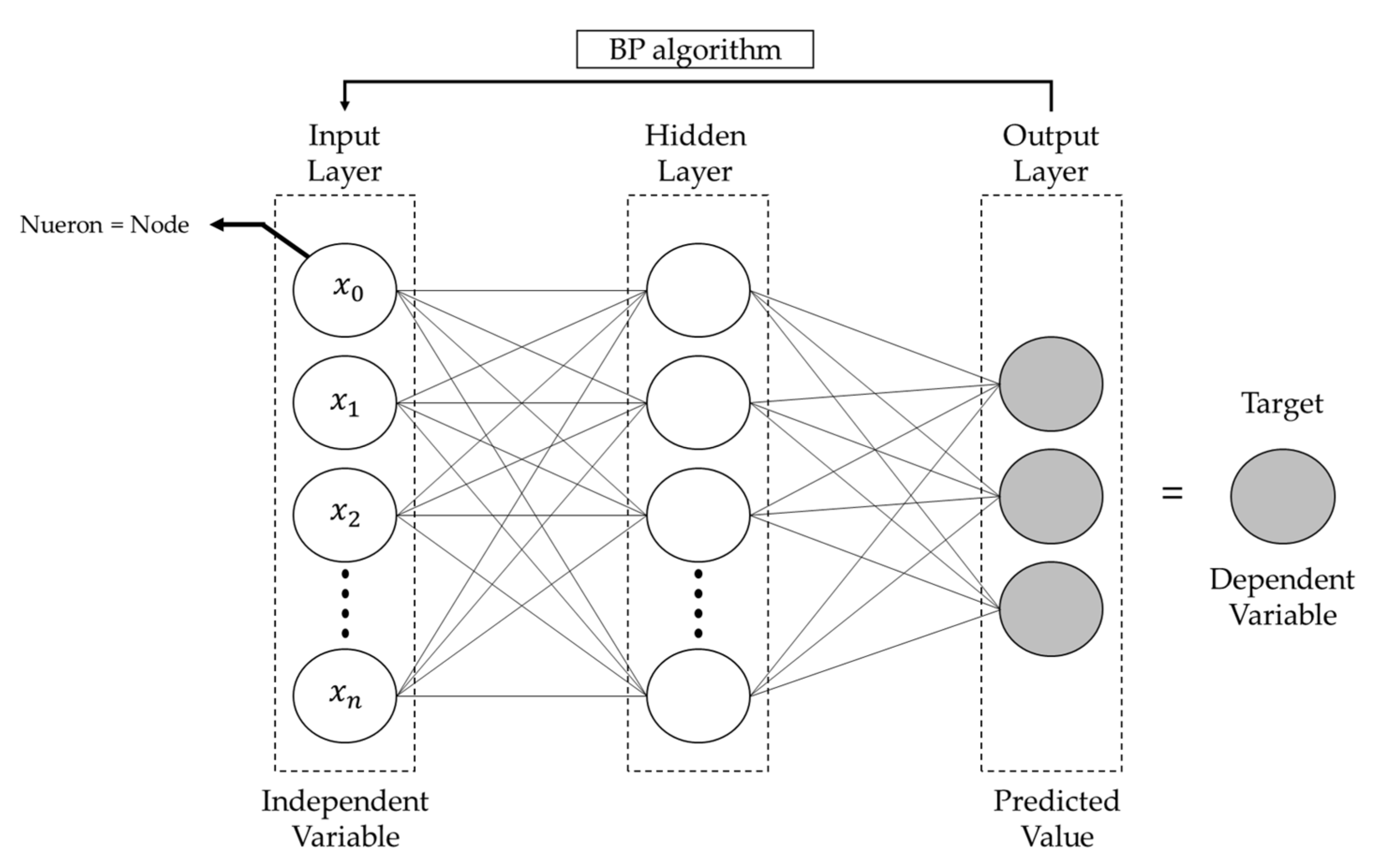
2.3. Artificial Neural Network
3. Model Comparison
4. Data Preparation
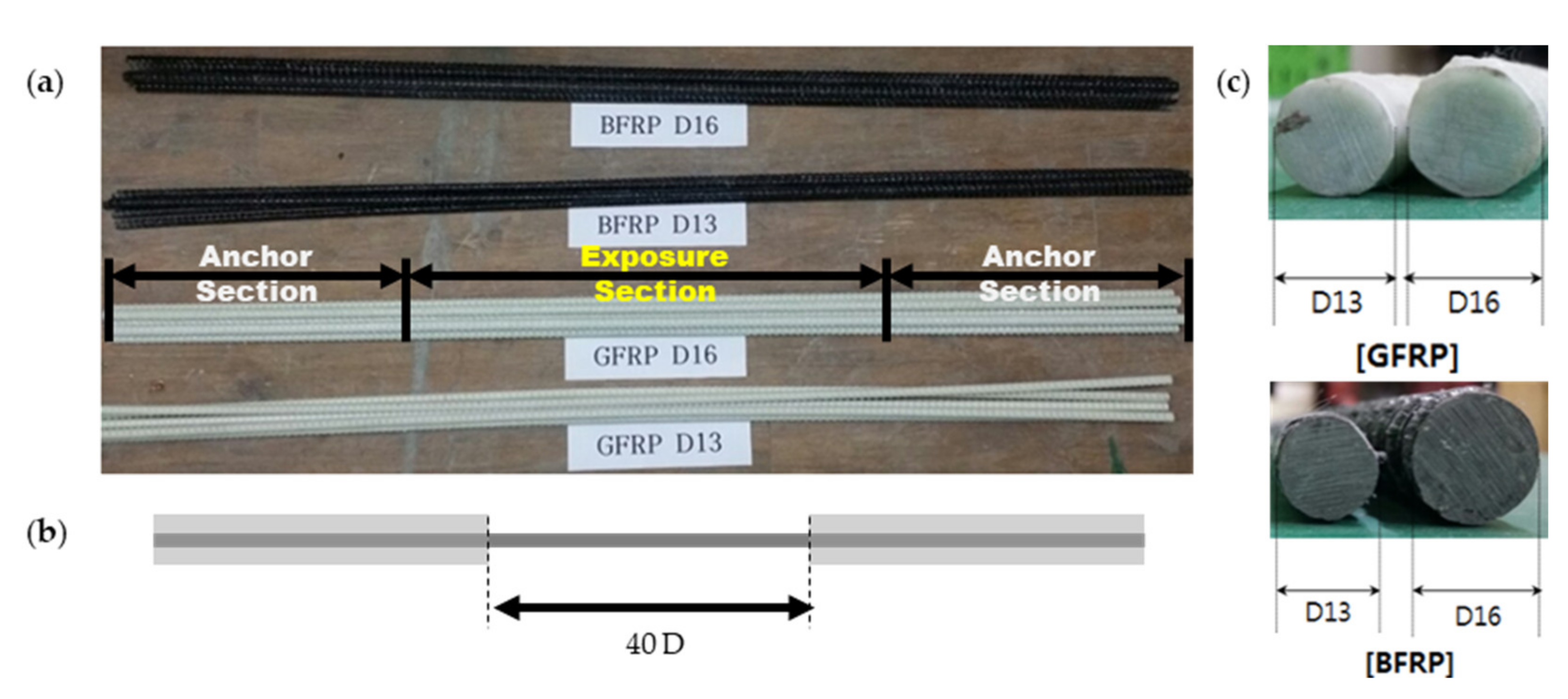
4.1. Test Specimens
4.2. Environmental Exposure Conditions
4.3. Tensile Test and Results
5. Analysis and Results
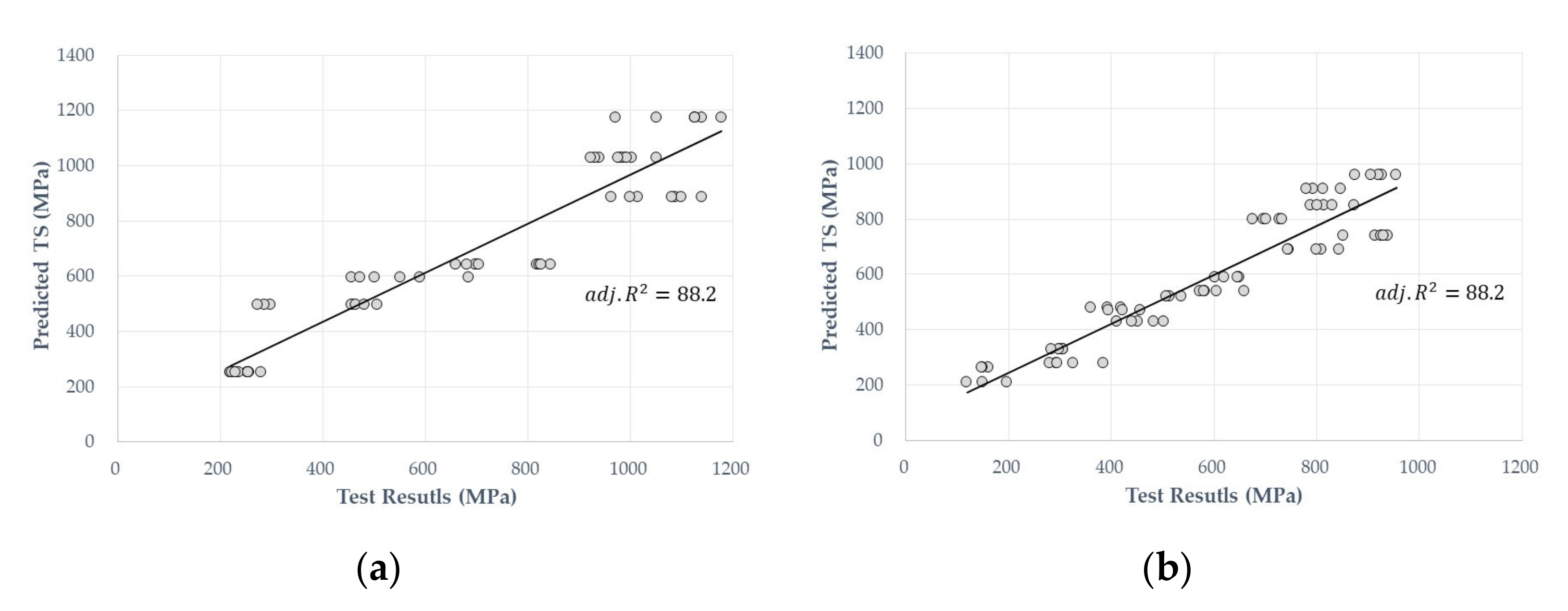
5.1. MRA Results
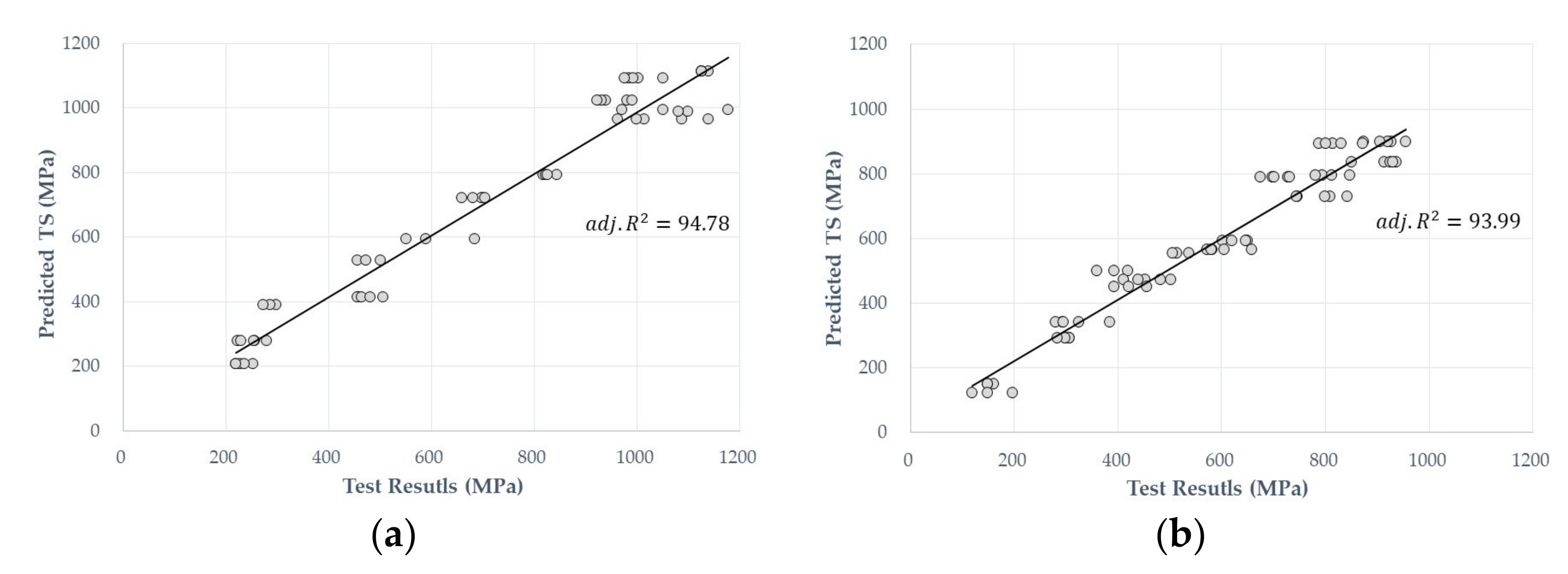
5.2. Polynomial Regression Analysis Results
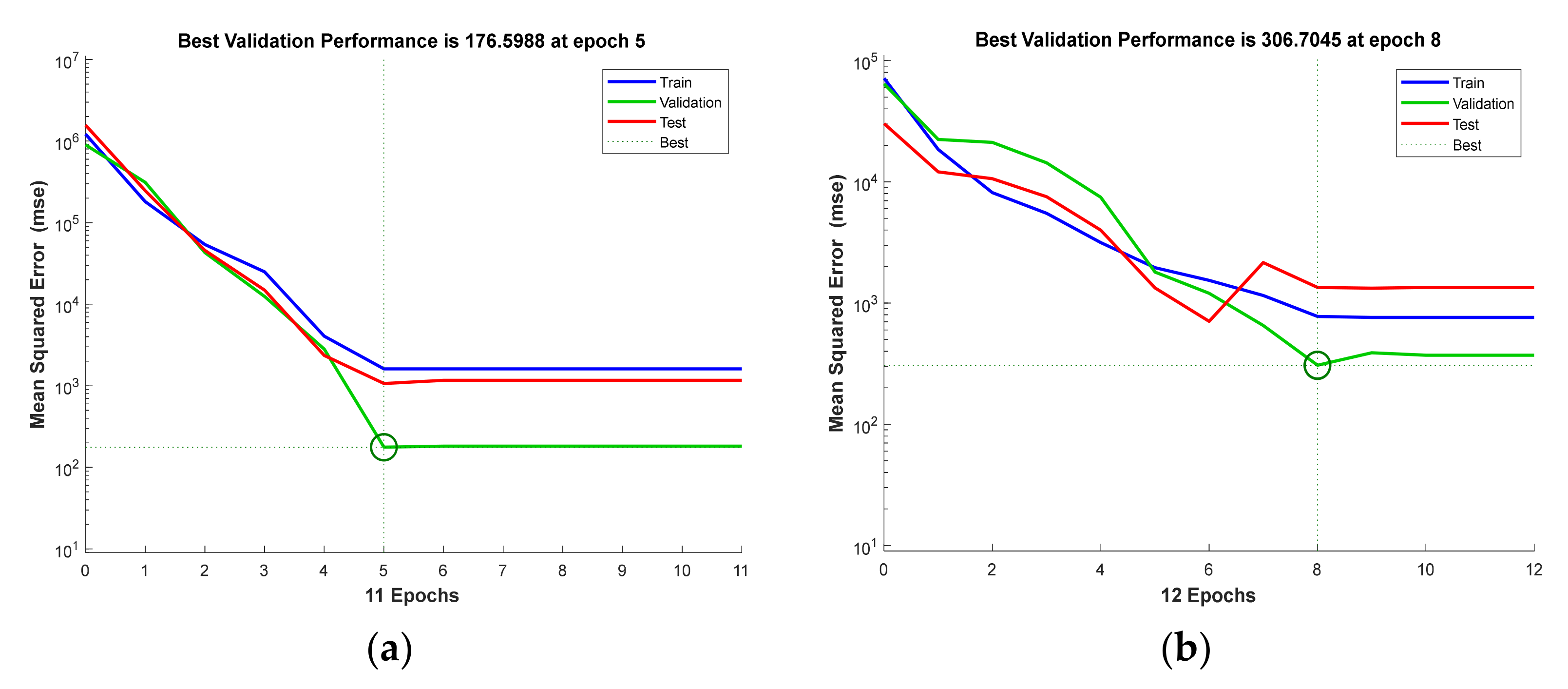
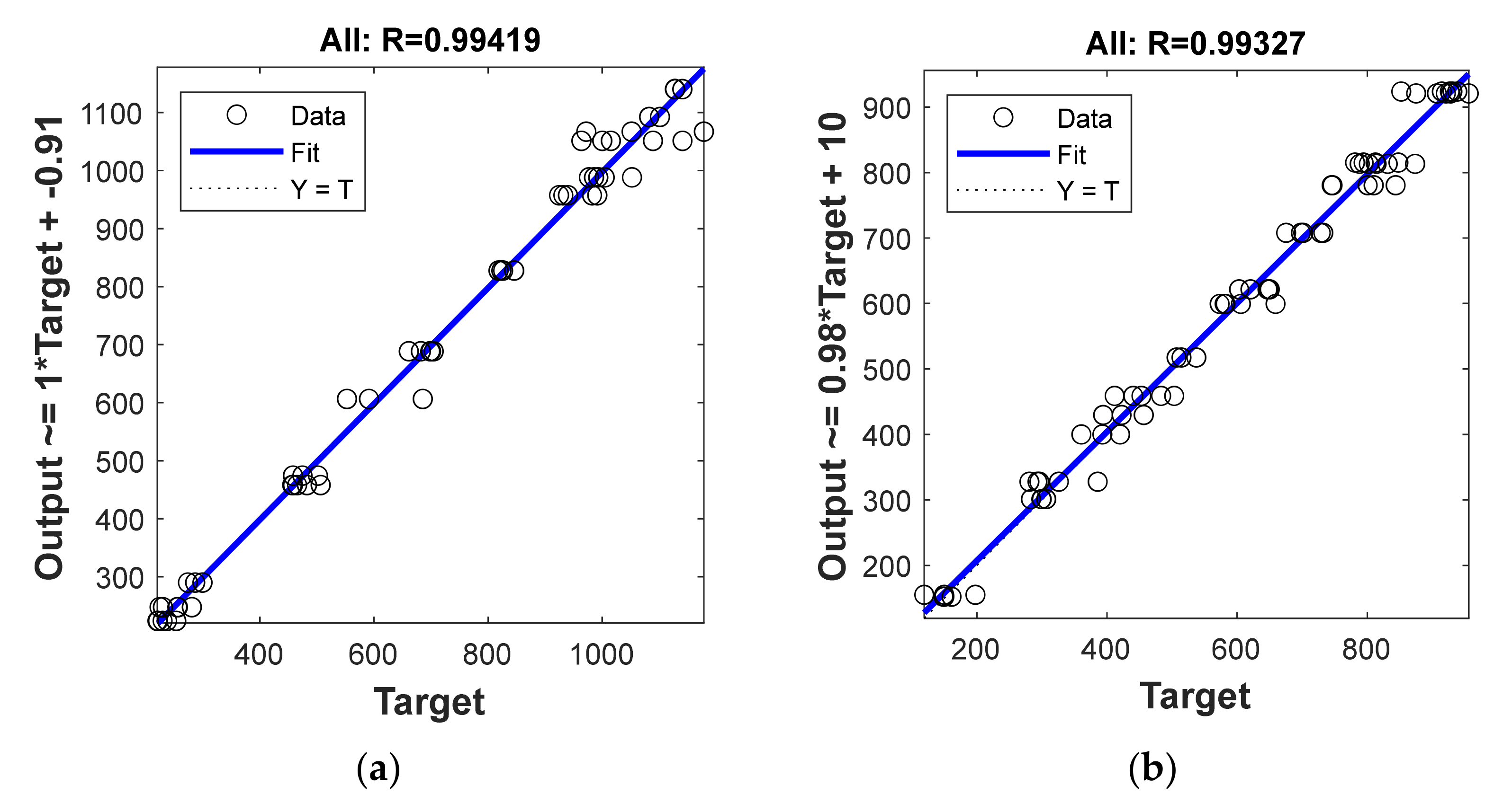
5.3. ANN Analysis Results
6. Summary and Discussion
7. Conclusions
Author Contributions
Funding
Institutional Review Board Statement
Informed Consent Statement
Data Availability Statement
Conflicts of Interest
References
- Berg, A.C.; Bank, L.C.; Oliva, M.G.; Russell, J.S. Construction and cost analysis of an FRP reinforced concrete bridge deck. Constr. Build. Mater. 2005, 20, 515–526. [Google Scholar] [CrossRef]
- Caratelli, A.; Meda, A.; Rinaldi, Z.; Spagnuolo, S.; Maddaluno, G. Optimization of GFRP reinforcement in precast segments for metro tunnel lining. Compos. Struct. 2017, 181, 336–346. [Google Scholar] [CrossRef]
- Berardi, U.; Dembsey, N. Thermal and Fire Characteristics of FRP Composites for Architectural Applications. Polymers 2015, 7, 2276–2289. [Google Scholar] [CrossRef] [Green Version]
- Wang, Z.; Zhao, X.L.; Xian, G.; Wu, G.; Raman, R.K.S.; Al-Saadi, S.; Haque, A. Long-term durability of basalt- and glass-fiber reinforced polymer (BFRP/GFRP) bars in seawater and sea sand concrete environment. Constr. Build. Mater. 2017, 139, 467–489. [Google Scholar] [CrossRef]
- Mugahed Amran, Y.H.; Alyousef, R.; Rashid, R.S.M.; Alabduljabbar, H.; Hung, C.C. Properties and applications of FRP in strengthening RC structures: A review. Structures 2018, 16, 208–238. [Google Scholar] [CrossRef]
- Davalos, J.F.; Chen, Y.; Ray, I. Long-term durability prediction models for GFRP bars in concrete environment. J. Compos. Mater. 2011, 46, 1899–1914. [Google Scholar] [CrossRef]
- Lu, Z.; Xian, G.; Li, H. Effects of elevated temperatures on the mechanical properties of basalt fibers and BFRP plates. Constr. Build. Mater. 2016, 127, 1029–1036. [Google Scholar] [CrossRef]
- Rifai, M.A.; El-Hassan, H.; El-Maaddawy, T.; Abed, F. Durability of basalt FRP reinforcing bars in alkaline solution and moist concrete environments. Constr. Build. Mater. 2020, 243, 118258. [Google Scholar] [CrossRef]
- Davalos, J.F.; Chen, Y.; Ray, I. Effect of FRP bar degradation on interface bond with high strength concrete. Cem. Concr. Compos. 2008, 30, 722–730. [Google Scholar] [CrossRef]
- Hollaway, L.C. A review of the present and future utilization of FRP composites in the civil infrastructure with reference to their important in-service properties. Constr. Build. Mater. 2010, 24, 2419–2445. [Google Scholar] [CrossRef]
- Ceroni, F.; Cosenza, E.; Gaetano, M.; Pecce, M. Durability issues of FRP rebars in reinforced concrete members. Cem. Concr. Compos. 2006, 28, 857–868. [Google Scholar] [CrossRef]
- Won, J.P.; Lee, S.J.; Kim, Y.J.; Jang, C.I.; Lee, S.W. The effect of exposure to alkaline solution and water on the strength-porosity relationship of GFRP rebar. Composites 2008, 39, 764–772. [Google Scholar] [CrossRef]
- Elgabbas, F.; Ahmed, E.A.; Benmokrane, B. Physical and mechanical characteristics of new basalt-FRP bars for reinforcing concrete structures. Constr. Build. Mater. 2015, 95, 623–635. [Google Scholar] [CrossRef]
- Benmokrane, B.; Ali, A.H.; Mohamed, H.M.; Elsafty, A.; Manalo, A. Laboratory assessment and durability performance of vinyl-ester, polyester, and epoxy glass-FRP bars for concrete structures. Compos. Part B 2017, 114, 163–174. [Google Scholar] [CrossRef] [Green Version]
- Tavakkol, S.; Alapour, F.; Kazemian, A.; Hasaninejad, A.; Ghanbari, A.; Ramezanianpour, A.A. Prediction of lightweight concrete strength by categorized regression, MLR and ANN. Comput. Concr. 2013, 12, 151–167. [Google Scholar] [CrossRef]
- Chithra, S.; Senthil Kumar, S.R.R.; Chinnaraju, K.; Alfin Ashmita, F. A comparative study on the compressive strength prediction models for High Performance Concrete containing nano silica and copper slag using regression analysis and Artificial Neural Networks. Constr. Build. Mater. 2016, 114, 528–535. [Google Scholar] [CrossRef]
- Atici, U. Prediction of the strength of mineral admixture concrete using multivariable regression analysis and an artificial neural network. Expert Syst. Appl. 2011, 38, 9609–9618. [Google Scholar] [CrossRef]
- Pranamika, R.; Senthil Pandian, M.; Karthikeyan, K. Predictive study on Mechanical strength of Lightweight concrete using MRA and ANN. Turk. J. Comput. Math. Educ. 2021, 12, 7774–7792. [Google Scholar] [CrossRef]
- Charhate, S.; Subhedar, M.; Adsul, N. Prediction of Concrete Properties using Multiple Linear Regression and Artificial Neural Network. J. Soft Comput. Civ. Eng. 2018, 2-3, 27–38. [Google Scholar] [CrossRef]
- Chopra, P.; Sharma, R.K.; Kumar, M. Regression Models for the Prediction of Compressive Strength of Concrete with & without Fly ash. Int. J. Latest Trends Eng. Technol. 2017, 3, 400–406. [Google Scholar]
- Alyamac, K.E.; Ghafari, E.; Ince, R. Development of eco-efficient self-compacting concrete with waste marble powder using the response surface method. J. Clean. Prod. 2017, 144, 192–202. [Google Scholar] [CrossRef]
- Haque, M.; Ray, S.; Mita, A.F.; Bhattacharjee, S.; Shams, M.J.B. Prediction and optimization of the fresh and hardened properties of concrete containing rice husk ash and glass fiber using response surface methodology. Case Stud. Constr. Mater. 2021, 14, e00505. [Google Scholar] [CrossRef]
- Li, W.; Cai, L.; Wu, Y.; Liu, Q.; Yu, H.; Zhang, C. Assessing recycled pavement concrete mechanical properties under joint action of freezing and fatigue via RSM. Constr. Build. Mater. 2018, 164, 1–11. [Google Scholar] [CrossRef]
- Habibi, A.; Ramezanianpour, A.M.; Mahdikhani, M.; Bamshad, O. RSM-based evaluation of mechanical and durability properties of recycled aggregate concrete containing GGBFS and silica fume. Constr. Build. Mater. 2021, 270, 121431. [Google Scholar] [CrossRef]
- Bezerra, M.A.; Santelli, R.E.; Oliveira, E.P.; Villar, L.S.; Escaleira, L.A. Response surface methodology (RSM) as a tool for optimization in analytical chemistry. Talanta 2008, 76, 965–977. [Google Scholar] [CrossRef] [PubMed]
- Naderpour, H.; Haji, M.; Mirrashid, M. Shear capacity estimation of FRP-reinforced concrete beams using computational intelligence. Structures 2020, 28, 321–328. [Google Scholar] [CrossRef]
- Zhou, Y.; Zheng, S.; Huang, Z.; Sui, L.; Chen, Y. Explicit neural network model for predicting FRP-concrete interfacial bond strength based on a large database. Compos. Struct. 2020, 240, 111998. [Google Scholar] [CrossRef]
- Nooraziah, A.; Janahiraman, T.V. A study on Regression Model Using Response Surface Methodology. Appl. Mech. Mater. 2014, 666, 235–239. [Google Scholar] [CrossRef]
- Sarle, W.S. Neural Networks and Statistical Models. In Proceeding of the Nineteenth Annual SAS Users Group International Conference, Cary, NC, USA, April 1994; pp. 1538–1550. [Google Scholar]
- McElroy, P.D.; Bibang, H.; Emadi, H.; Kocoglu, Y.; Hussain, A.; Watson, M.C. Artificial neural network (ANN) Approach to predict unconfined compressive strength (UCS) of oil and gas well cement reinforced with nanoparticles. J. Nat. Gas Sci. Eng. 2021, 88, 103816. [Google Scholar] [CrossRef]
- Dai, L.; He, X. Experimental Study on Tensile Properties of GFRP Bars Embedded in Concrete Beams with Working Cracks. MATEC Web Conf. 2017, 2005. [Google Scholar] [CrossRef] [Green Version]
- Kazakevich, T.; Mamodov, S.; Nizhegorodtsev, D.; Klevan, V. Improving the reliability of FRP bars tests by increasing the adhesive strength in Specimen anchor. IOP Conf. Ser. Mater. Sci. Eng. 2020, 896, 012033. [Google Scholar] [CrossRef]
- Brahim, B.; Claude, N.; Xavier, S.; Allan, M. Comparison between ASTM D7205 and CSA S806 Tensile-Testing Methods for Glass Fiber-Reinforced Polymer Bars. J. Compos. Constr. 2017, 21, 5. [Google Scholar] [CrossRef]
- Zhou, Q.; Wang, F.; Zhu, F. Estimation of compressive strength of hollow concrete masonry prisms using artificial neural networks and adaptive neuro-fuzzy inference. Constr. Build. Mater. 2016, 125, 417–426. [Google Scholar] [CrossRef]
- Nazerian, M.; Kamyabb, M.; Shamsianb, M.; Dahmardehb, M.; Kooshaa, M. Comparison of response surface methodology (RSM) and artificial neural networks (ANN) towards efficient optimization of flexural properties of gypsum-bonded fiberboards. Open Sci. J. 2018, 24, 35–47. [Google Scholar] [CrossRef]
- Xu, W.S.; Yu, Q.M.; Sun, Y.L.; Dong, T.W. Research on Improving Training Speed of LMBP Algorithm and its Simulation in Application. In Proceedings of the International Conference on Computational Intelligence and Security, Harbin, China, 15–19 December 2007; pp. 540–545. [Google Scholar] [CrossRef]
- Badkar, D.S.; Pandey, K.S.; Buvanashekaran, G. Development of RSM- and ANN-based models to predict and analyze the effects of process parameters of laser-hardened commercially pure titanium on heat input and tensile strength. Int. J. Adv. Manuf. Technol. 2013, 65, 1319–1338. [Google Scholar] [CrossRef]
- Oh, H.; Kim, Y.; Jang, N. An Experimental Study on the Degradations of Material Properties of Vinylester/FRP Reinforcing Bars under Accelerated Alkaline Condition. J. Korea Inst. Struct. Maint. Insp. 2019, 23, 51–59. [Google Scholar] [CrossRef]


| Exposure Condition | TP (°C) | ED (Days) |
|---|---|---|
| Reference | In air | - |
| Alkaline solution (pH = 12.6) | 20, 40, 60 | 50 |
| 100 | ||
| 200 |
| D (mm) | TP (°C) | ED (Days) | Tensile Strength (MPa) Average ± SD | |
|---|---|---|---|---|
| BFRP | GFRP | |||
| 13 | 20 | 0 | 1067.2 ± 84.86 | 917.30 ± 26.48 |
| 20 | 50 | 953.9 ± 27.40 | 821.97 ± 29.39 | |
| 40 | 50 | 689.3 ± 16.02 | 633.80 ± 18.87 | |
| 60 | 50 | 232.4 ± 12.18 | 299.15 ± 8.59 | |
| 20 | 100 | 1041.7 ± 64.17 | 912.50 ± 31.14 | |
| 40 | 100 | 286.6 ± 10.46 | 391.27 ± 24.34 | |
| 20 | 200 | 609.7 ± 55.78 | 519.58 ± 12.90 | |
| 40 | 200 | - | 153.33 ± 5.56 | |
| 16 | 20 | 0 | 1130.73 ± 5.61 | 808.95 ± 25.07 |
| 20 | 50 | 1002.37 ± 26.49 | 707.16 ± 21.09 | |
| 40 | 50 | 828.40 ± 10.40 | 600.18 ± 31.40 | |
| 60 | 50 | 249.33 ± 20.41 | 316.37 ± 37.79 | |
| 20 | 100 | 1091.72 ± 9.46 | 789.18 ± 38.12 | |
| 40 | 100 | 473.76 ± 18.79 | 458.30 ± 32.11 | |
| 20 | 200 | 478.06 ± 18.08 | 424.37 ± 25.48 | |
| 40 | 200 | - | 155.68 ± 32.38 | |
| Type | Variable | t | p | TOL | VIF | |
|---|---|---|---|---|---|---|
| BFRP | Constant | 1561.94 | 34.962 | 0.000 | - | - |
| TP | −19.409 | −19.491 | 0.000 | 0.963 | 1.039 | |
| ED | −2.887 | −10.109 | 0.000 | 0.963 | 1.039 | |
| D | - | 0.864 | 0.391 | 0.998 | ||
| F(p) | 210.862 | 0.942 | ||||
| 0.882 | 0.886 | |||||
| Durbin–Watson | 0.863 | p-value | 0.000 | |||
| GFRP | Constant | 1439.72 | 14.173 | 0.000 | - | - |
| TP | −12.99 | −18.441 | 0.000 | 0.997 | 1.003 | |
| ED | −2.19 | −13.353 | 0.000 | 0.997 | 1.003 | |
| D | −17.0 | −2.509 | 0.015 | 0.998 | 1.002 | |
| F(p) | 169.626 | 0.942 | ||||
| 0.882 | 0.887 | |||||
| Durbin–Watson | 0.594 | p-value | 0.000 | |||
| BFRP Terms | Contribution | F-Value | p-Value | GFRP Terms | Contribution | F-Value | p-Value |
|---|---|---|---|---|---|---|---|
| TP | 67.17 | 4.33 | 0.043 | TP | 56.14 | 36.89 | 0.000 |
| ED | 21.48 | 25.65 | 0.000 | ED | 31.43 | 5.71 | 0.020 |
| D | 0.16 | 12.25 | 0.001 | D | 1.10 | 25.35 | 0.000 |
| 0.08 | 13.50 | 0.001 | 3.76 | 28.85 | 0.000 | ||
| 1.31 | 28.40 | 0.000 | 0.79 | 9.38 | 0.003 | ||
| TP*ED | 4.65 | 49.31 | 0.000 | TP*ED | 1.29 | 14.61 | 0.000 |
| ED*D | 0.58 | 6.19 | 0.016 | ED*D | - | - | - |
| 97.68 | 97.22 | ||||||
| 95.43 | 94.52 | ||||||
| 94.78 | 93.99 | ||||||
| Durbin–Watson | 1.265 | Durbin–Watson | 0.783 | ||||
| Training | Validation | Testing | NN Model | |||||
|---|---|---|---|---|---|---|---|---|
| MSE | MSE | MSE | MSE | |||||
| BFRP | 0.991 | 1617.3 | 0.999 | 176.6 | 0.995 | 1069.2 | 0.994 | 1233.5 |
| GFRP | 0.993 | 774.2 | 0.996 | 306.7 | 0.990 | 1345.4 | 0.993 | 795.2 |
| MRA | PRA | ANN | ||||
|---|---|---|---|---|---|---|
| BFRP | GFRP | BFRP | GFRP | BFRP | GFRP | |
| 0.94 | 0.94 | 0.98 | 0.97 | 0.99 | 0.99 | |
| RMSE | 109.24 | 81.86 | 69.32 | 56.94 | 35.12 | 28.20 |
| MAE | 82.31 | 66.48 | 56.03 | 45.39 | 24.00 | 22.19 |
| MAPE | 13.51 | 14.33 | 9.60 | 8.50 | 3.71 | 4.68 |
Publisher’s Note: MDPI stays neutral with regard to jurisdictional claims in published maps and institutional affiliations. |
© 2021 by the authors. Licensee MDPI, Basel, Switzerland. This article is an open access article distributed under the terms and conditions of the Creative Commons Attribution (CC BY) license (https://creativecommons.org/licenses/by/4.0/).
Share and Cite
Kim, Y.; Oh, H. Comparison between Multiple Regression Analysis, Polynomial Regression Analysis, and an Artificial Neural Network for Tensile Strength Prediction of BFRP and GFRP. Materials 2021, 14, 4861. https://doi.org/10.3390/ma14174861
Kim Y, Oh H. Comparison between Multiple Regression Analysis, Polynomial Regression Analysis, and an Artificial Neural Network for Tensile Strength Prediction of BFRP and GFRP. Materials. 2021; 14(17):4861. https://doi.org/10.3390/ma14174861
Chicago/Turabian StyleKim, Younghwan, and Hongseob Oh. 2021. "Comparison between Multiple Regression Analysis, Polynomial Regression Analysis, and an Artificial Neural Network for Tensile Strength Prediction of BFRP and GFRP" Materials 14, no. 17: 4861. https://doi.org/10.3390/ma14174861
APA StyleKim, Y., & Oh, H. (2021). Comparison between Multiple Regression Analysis, Polynomial Regression Analysis, and an Artificial Neural Network for Tensile Strength Prediction of BFRP and GFRP. Materials, 14(17), 4861. https://doi.org/10.3390/ma14174861