Article

Using Artificial Neural Networks to Predict Influences of Heterogeneity on Rock Strength at Different Strain Rates

School of Civil Engineering, The University of Sydney, Sydney, NSW 2006, Australia
*
Author to whom correspondence should be addressed.
Materials 2021, 14(11), 3042; https://doi.org/10.3390/ma14113042
Submission received: 18 April 2021 / Revised: 15 May 2021 / Accepted: 1 June 2021 / Published: 3 June 2021

Abstract

:
Pre-existing cracks and associated filling materials cause the significant heterogeneity of natural rocks and rock masses. The induced heterogeneity changes the rock properties. This paper targets the gap in the existing literature regarding the adopting of artificial neural network approaches to efficiently and accurately predict the influences of heterogeneity on the strength of 3D-printed rocks at different strain rates. Herein, rock heterogeneity is reflected by different pre-existing crack and filling material configurations, quantitatively defined by the crack number, initial crack orientation with loading axis, crack tip distance, and crack offset distance. The artificial neural network model can be trained, validated, and tested by finite 42 quasi-static and 42 dynamic Brazilian disc experimental tests to establish the relationship between the rock strength and heterogeneous parameters at different strain rates. The artificial neural network architecture, including the hidden layer number and transfer functions, is optimized by the corresponding parametric study. Once trained, the proposed artificial neural network model generates an excellent prediction accuracy for influences of high dimensional heterogeneous parameters and strain rate on rock strength. The sensitivity analysis indicates that strain rate is the most important physical quantity affecting the strength of heterogeneous rock.

1. Introduction

Natural rocks typically have substantial heterogeneity in terms of containing pre-existing flaws at multiple scales resulting from a variety of geological processes. The heterogeneity makes alternations to rock mechanical strength, further affecting the deformation behaviors and failure patterns upon loading [1,2]. In fact, to a certain degree, almost all rock-related engineering projects include structure constructions in rock masses, which involve pre-existing opening cracks [3,4]. For example, human excavations can greatly alter the stability of rock masses as a result of disturbance of the primary stress equilibrium, leading to artificially induced stress redistribution. Consequently, stress concentration may occur around the pre-existing flaws, which triggers crack coalescence and ultimate failure [5,6]. These opening flaws are usually naturally filled with different fine-grained materials due to weathering or joint shearing [7]. In geological constructions, opening flaws are manually filled via grouting and shotcrete to strengthen the load capacity of flawed rocks [8,9]. The addition of filling materials further enhances the rock heterogeneity. Fracture behaviors of flawed rock become more complex with the involvement of filling materials due to the complicated interactions between rock and flaw filling. In addition, natural rocks are often subjected to high strain rate loadings, such as earthquakes, rock blasting and oil-well fracturing. As a rate-dependent material, the heterogeneous rock mechanical strength is also highly related to the strain rate [10].
Hence, it is vital to establish the relationship between the heterogeneity on the flawed rock (induced by pre-existing flaws and filling materials) concerning the mechanical strength at different strain rates, bringing great convenience to rock engineering application and geotechnical design. In terms of evaluating the rock mechanical strength, laboratory tests are the most widely applied direct approaches, where standardized specimens are indeed required according to the corresponding testing standards. So far, several laboratory experiments have been performed on the flawed rocks with different pre-existing crack configurations, such as crack geometry, number, orientation, etc. [11,12]. For instance, by performing static and dynamic experiments on cubic rock specimens with a single pre-existing flaw, Yan et al. [13] illustrated the significant coupled effects of pre-compression and strain rate on rock strength and fracture responses. Zhao et al. [14] investigated the cracking and coalescence modes on the rock-like specimen containing two parallel cracks via uniaxial compression tests. They highlighted that the peak strength of the tested samples is related to the crack inclination angle and the associated bridge angle. In addition, Huang et al. [15] put more emphasis on probing into the effects of confining pressures. Regarding three pre-existing fissures, Zhou et al. [16] focused on the investigation of coupled thermomechanical and underlying cracking mechanisms. However, the major drawbacks of experiments are also obvious; they are known to be time-consuming and expensive. Considering the multiple heterogeneous parameters and strain rate that influence the mechanical behaviors of the flawed rock, a large number of samples with variations are required. For some special fragile or heavily weathered rocks, an adequate number of high-quality formed samples is not always feasible to obtain. Therefore, laboratory-based rock mechanical strength estimation may be problematic, especially for investigating high dimensional variables.
An alternative approach is to run numerical simulations by performing parametric studies to reduce the excessive experimental workload and cut the unnecessary cost [17,18]. For example, Wang et al. [19] performed extended finite element method simulation to investigate the initiation mechanisms of wing cracks, which stayed consistent with the theoretical analysis. Liu et al. [20] incorporated a fluid coupled model into grain-based model to discover the promotion mechanisms for crack coalescence in two systems with pre-existing flaws. Shen et al. [21] adopted a discrete element method to establish the relationships between P wave velocity and the number of pre-existing cracks, as well as confining pressure. However, as an indirect approach, the simulation study has its inherent disadvantages. Before conducting simulation, a thorough understanding is needed, with an awareness of all the factors involved. Meanwhile, a considerable amount of time is spent on validating the material constitutive parameters. Other conventional method is either seeking an analytical solution or obtaining the empirical solution for simplicity and reliability [22]. Nevertheless, these two options are not always achievable for complicated problems involving nonlinear and high-dimensional variables [23].
Recently, the artificial neural network (ANN) approach has shown promising capabilities in handling the abovementioned complex problem [24,25]. The ANN-based approach presented more reliable and acceptable results than conventional statistical analysis, as reported in [26]. ANN has an inherent ability to learn from available datasets and has been proven to be a powerful tool in various fields. For example, Gope et al. [27] designed an efficient ANN architecture to predict the crack growth direction of aluminum alloys. Liu and Athanasiou [23] successfully captured the complex relationship among the plane–strain stress intensity factor, the indentation load, and the specimen dimensions through ANN. Yan et al. [28] proved that ANN models are viable for predicting fracture parameters with high accuracy by using only 77 sets of experimental data. For predicting the rock strength, the previous ANN models primarily take the inherent physical properties of rock materials into account, e.g., porosity [29], P wave velocity [29], unit weight [30] and point load index [29,30]. Some of the input parameters considered, such as lithology, are only qualitatively introduced into the neural network [30]. However, limited attention was paid to forecasting the influences of the rock heterogeneity on rock strength by the ANN approach. In addition, the strain rate effect was also ignored in the previous ANN-based models despite its importance.
Targeting the gaps in the existing literature, this study adopts the ANN approach to predict the influences of heterogeneity on rock strength at different strain rates. The ANN model is implemented in Matlab (R2020a). The raw dataset is collected from our previous 84 Brazilian disc tests [31,32,33]. In these tests, 3D-printed Brazilian disc specimens with pre-existing single and double flaws were compressed under quasi-static and dynamic loadings. The application of the 3D printing technique can eliminate the creation of micro cracks and guarantee the imprecise flaws in the geometry during the flaw embedding process, making the experimental results more reliable. The considered heterogeneous parameters in this study include the flaw number, relative flaw location, flaw orientation, and strain rate. The optimization of the ANN architecture is performed using a trial-and-error method in terms of transfer functions and hidden neuron numbers. The predictions obtained from the trained ANN model are compared with the experiments to evaluate ANN model performance. In addition, a sensitivity study demonstrates the relative importance of the individual input variable, and the effects of different input numbers are also investigated.

2. Methodology

As a versatile approach for dealing with nonlinear problems, the artificial neural network (ANN) is in the form of a multilayer network, consisting of two propagation directions, namely feed forward and back propagation [24]. As shown in Figure 1, a typical ANN architecture is divided into three parts: one input layer, one or multiple hidden layers, and one output layer. Multiple layers containing different numbers of neurons are connected by either nonlinear or linear transfer functions. The complex nonlinear relationship between input and output variables can be learned via these transfer functions. The collection of neuron nodes distributed in each layer has their unique weight and bias values to describe the interconnection strength within the network. In Figure 1, [ I W 1 ] and [ I W 2 ] represent the input weight matrixes, while [ b 1 ] and [ b 2 ] represent the bias matrixes in the hidden and output layers, respectively.
Herein, the updating of the weight and bias matrixes is achieved by adopting the Levenberg–Marquardt algorithm as the training function. As a typical backpropagation algorithm, the Levenberg–Marquardt optimization has its inherent advantages, pertaining to convergence rate, generalization performance and precision, although more memory is required [34]. Since the Levenberg–Marquardt algorithm is an iterative procedure, the application of training function is a process of adjusting the network weight and bias matrixes for each epoch. The initial weight and bias values are random, and there is no need to make a prior assumption. The algorithm implementation has two phases. Firstly, input variables are propagated forward through the network via transfer functions to emerge as output variables, defined as a feed-forward process. To assess the ANN model performance, the averaged squared difference between the outputs and targets is proposed and quantified by a mean square error (MSE):
M S E = 1 n i = 1 n ( O i T i ) 2
Meanwhile, the correlation between the outputs and targets is expressed by a regression value R as:
R 2 = 1 1 n ( O i T i ) 2 1 n O i 2
where n is the number of outputs, and O i and T i are the ith output and target values, respectively.
During training, if the MSE meets the target error, the training process is then terminated because the predictive accuracy is sufficient. Otherwise, the error between the predicted output and target output values will be propagated backward through the network to update the connection weights and biases, in order to minimize the errors, until the MSE satisfies the target error. This is the second phase, also known as the backpropagation process. The detailed derivation of the Levenberg–Marquardt algorithm can be found in previous literature [35,36].
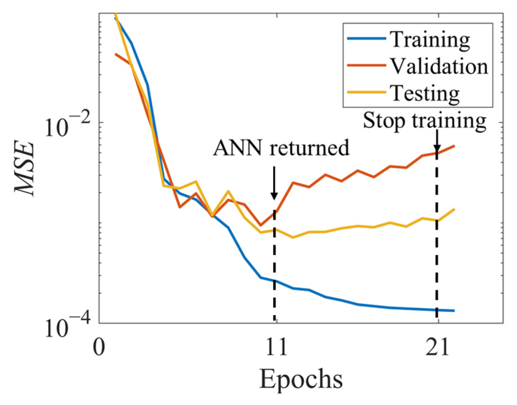
To avoid overfitting and increase the generalization capability of the trained ANN, an early stopping technique is utilized during the training procedure. The entire dataset is divided into three subsets, namely, the training set, the validation set and the testing set. During the training procedure, the first two datasets are used. The training set is used for computing and updating the network weights and biases. During the training process, as with the training error, the model performance on the validation set is simultaneously monitored. When the validation error starts to increase for a certain number of iterations (set as 10 here), the training is terminated. The increase in the validation error indicates the decrease in the model generalization ability. The entire network will then return the weight and bias matrixes when the overall error is at its minimum.

2.1. Input and Output Variables

The current study aims to investigate the ANN application in establishing the relationship between the rock strength (peak load) and rock heterogeneous factors at different strain rates. An experimental dataset including 84 Brazilian disc experiments has been collected from our previous studies [31,32,33]. For the multiple-crack system, descriptive and appropriate crack geometric parameters should be properly selected, which is vital to obtain an acceptable predictive accuracy with a relatively small dataset. Herein, the selected parameters include (1–2) the crack inclination angle with loading axis α 1 , α 2 , where the subscripts are used to distinguish the different flaws; (3) the crack offset distance H ; (4) the crack tip distance S , (5–6) the flaw filling f 1 , f 2 , and (7) the strain rate ε ˙ , as shown in Figure 2a. These seven parameters construct the input variables, and the peak load PL, as marked in Figure 2b, is the output variable. The entire dataset containing 84 experiments is listed in Table A1 in Appendix A. For the single flaw tests, H and S are equal to 0. If the open flaw is filled, its corresponding filling parameter is set as 1; otherwise, it will be 0.
The raw dataset can be normalized on a scale of 0 to 1 to improve the network performance. The normalization equation is given as follows:
x i N = x i O x m i n x m a x x m i n
where x i N and x i O are the ith normalised and original variable values, respectively. x m i n and x m a x are the minimal and maximum values of the variable set.

2.2. Optimization of ANN

In this application, the trial-and-error method is adopted for optimizing the network structure and operational parameters because of the small dataset and low computational consumption for each trial [27]. Different transfer function combinations and the min–max normalization effect are tuned in order to find the best setting. Meanwhile, a parametric study for hidden layer neuron number is conducted.
For better comparison, different ANNs are required to be performed on the same training, validation and testing dataset divisions, accounting for 60, 12 and 12 out of the total 84 experiments, respectively. To be specific, the validation dataset contains Test No. 5, 13, 15, 23, 32, 42, 49, 53, 58, 64, 76, 82, the testing dataset contains the Test No. 6, 12, 17, 25, 35, 37, 44, 52, 62, 68, 70, 80, while the rest belongs to the training dataset. Since the network is trained to start from different initial weights and biases, this may lead to different solutions even for the same dataset division. Each ANN structure is trained ten times and the ANN with the best performance is selected. The MSE or R values for the training and testing dataset are chosen to evaluate the training and generalization performances, respectively. The ANN, owing the smaller average MSE or the larger average R, is considered to have better performance.

2.2.1. Transfer Functions

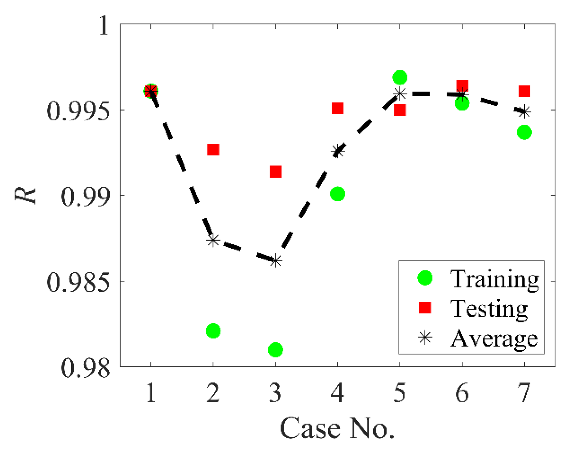
Based on the previous studies [28,37], one hidden layer is applied due to the limited input and output variables. The network with too many hidden layers or neurons can be easily over-trained and will not sufficiently predict the new data. The detailed analysis of the neuron number contained in the hidden layer is elaborated in the subsequent section. The different setting combinations are performed on the same 7-10-1 ANN, where the ANN contains 10 hidden layer neurons. Table 1 lists seven different transfer functions and normalization setting combinations. Figure 3 presents the regression values for different ANN settings.
As shown in Figure 3, the setting of case 1 is superior to other cases and the following study adopted same transfer functions and normalization setting. It should also be noted that, for cases 2, 3 and 4, the trained ANNs present a better testing accuracy than the training results, which may result from the fixed data set splitting here. Although these three cases have poor training accuracy for the training dataset, the trained ANNs appear to be more suitable for the testing dataset, leading to a higher regression value [27].

2.2.2. Hidden Layer Neuron Number

Yan et al. [28] reported the following formulation to estimate the neuron number in the single hidden layer:
m = n + l + a
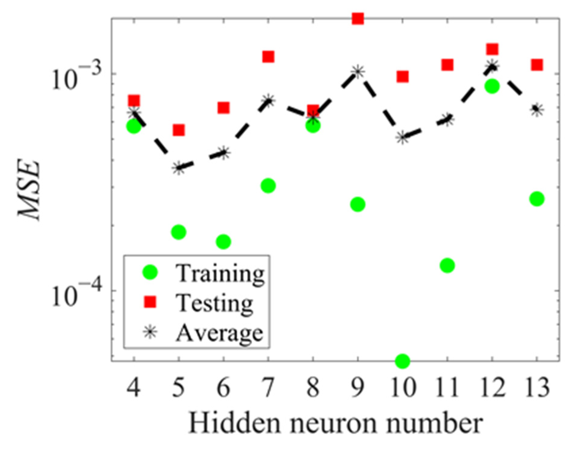
where m ,   n and l the neuron numbers of hidden, input and output layers, respectively. a is a constant, ranging from 1 to 10. The neurons number in the hidden layers is investigated in the range of 4 to 13. The comparison between different ANNs is also performed for the same abovementioned dataset divisions and the MSE values for each case are shown in Figure 4. The training MSE is usually smaller than the testing MSE. The neuron number in the hidden layer is chosen to be 5 since this leads to a relatively smaller average MSE value.

2.3. ANN Training

Table 2 provides the ANN setting after optimization. The training is repeated 10 times and the ANN with the best performance is selected.
The training procedure of the picked ANN is illustrated in Figure 5. After epoch-11, the error of the validation starts to increase, as well as that of the testing dataset. Although the training accuracy is still increasing, the generalization ability tends to decrease. As a result, the training stops at epoch-21 and returns the training value at epoch-11 due to the early stopping setting. The outcome of the chosen ANN is shown in Figure 6. It is observed that the R values for training, validation and testing are 0.9962, 0.9863, and 0.9983, respectively. The overall regression value R is 0.9951.
The weights and biases associated with this trained ANN are given as follows:
[ I W 1 ] = [ 1.4976 0.5617 0.5583 0.0933   0.4677   0.6805   0.4803 0.4817   0.5290   0.9578 0.5081   0.6548   0.2266 0.5202 0.7050 0.5152 0.3833   0.1897   1.2370 0.0207   2.2187 0.5221 0.2058 0.9680 1.1084   0.0890   0.2536 1.1518 0.2287   0.6957   0.3462 0.4682   0.8604   0.0799   2.0323 ] [ I W 2 ] T = [ 0.3040 0.6847 0.7211 0.5353 0.1036 ] [ b 1 ] T = [ 1.5586 0.9090 0.0191 1.4385 1.2869 ] [ b 2 ] T = [ 0.6196 ]

3. Results and Discussion

The entire dataset is used to evaluate the accuracy of the predicted peak load by the ANN approach. All predicted results by the trained ANN are listed in Appendix A. The importance factors of each input variable on the peak load are calculated by the sensitivity analysis.

3.1. Predicting Results

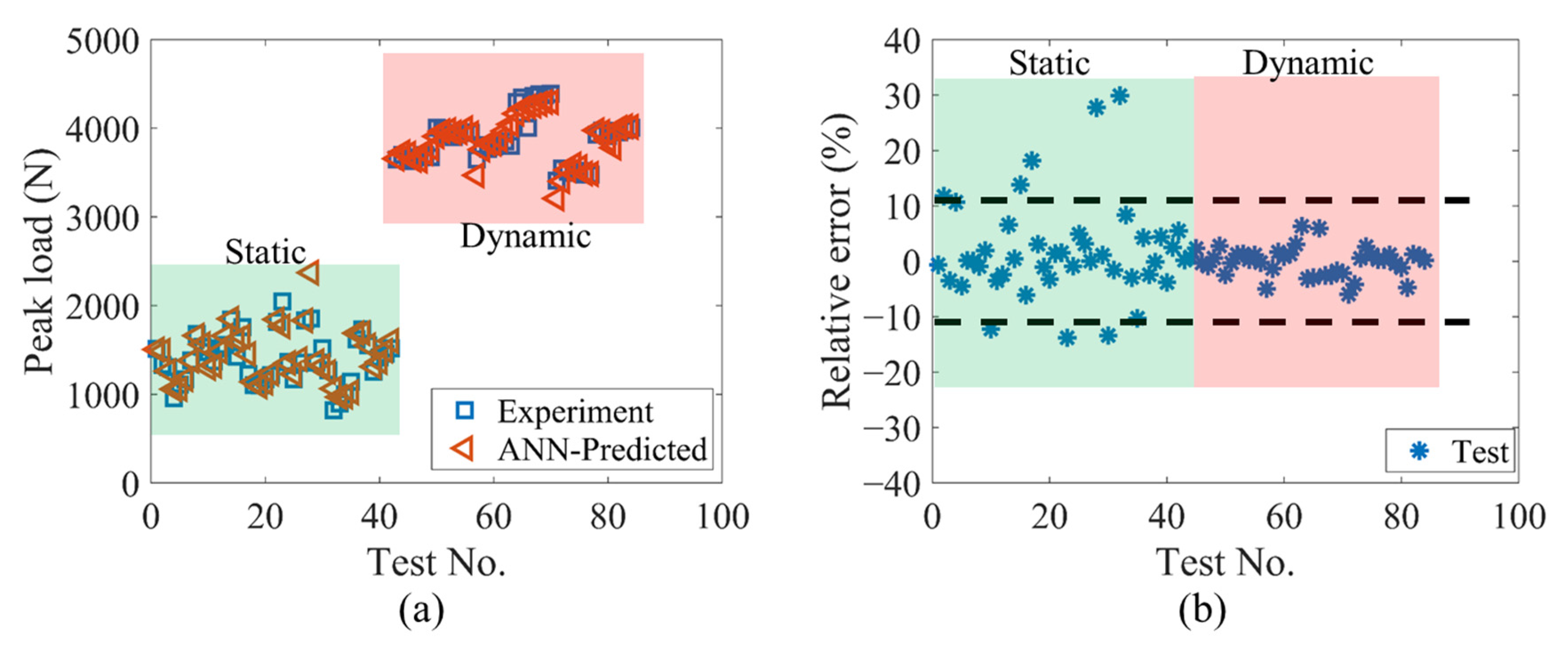
Figure 7a presents a comparison of the peak loads predicted by the ANN model with the experimental results, and Figure 7b shows the relative error values between the ANN-predicted and experimental results. The relative error is calculated as ( P L A N N P L E x p e r i m e n t ) / P L E x p e r i m e n t , where P L A N N and P L E x p e r i m e n t are the ANN predicted and experimental results, respectively. Meanwhile, the statistical analysis based on the ratio of P L A N N / P L E x p e r i m e n t and mean absolute relative error is performed, and the key descriptive statistics are summarized in Table 3.
It is clear that the dynamic test section has better predicted results than the static test section in terms of mean, standard deviation (SD) and coefficient of variation (COV) for the ratio of P L A N N / P L E x p e r i m e n t , as well as a smaller mean absolute relative error. Except for several data points in the static test section, the majority of the predicted data have a relative error within ±10%.
Generally speaking, the ANN model demonstrates its strong ability to quickly (within seconds) and accurately predict the peak load. The current trained ANN model has a good mean value (close to 1) and a small standard deviation, indicating that the ANN model has a good generalization ability. In addition, the relatively small COV value indicates fewer scattering results. The overall mean absolution relative error is only 4.49%.

3.2. Sensitivity Analysis

To quantify the relative influence factor of each input variable on the peak load, Garson’s equation, derived from neuron weight matrixes (IW1 and IW2), is applied, as illustrated below [38,39]:
I i k = j = 1 L ( ( | I W 1 i j | i = 1 N | I W 1 i j | ) × | I W 2 j k | ) i = 1 N ( j = 1 L ( ( | I W 1 i j | i = 1 N | I W 1 i j | ) × | I W 2 j k | ) )
where I i k is the relative importance factor of the ith input neuron on the kth output neuron, N and L are the numbers of input and hidden neurons, respectively, I W 1 i j is the connection weight matrix between the ith input neuron and the jth hidden neuron, while I W 2 j k is the connection weight matrix between the jth hidden neuron and the kth output neuron. Note that the ANN model is obtained based on a series of min–max normalized inputs and output data.
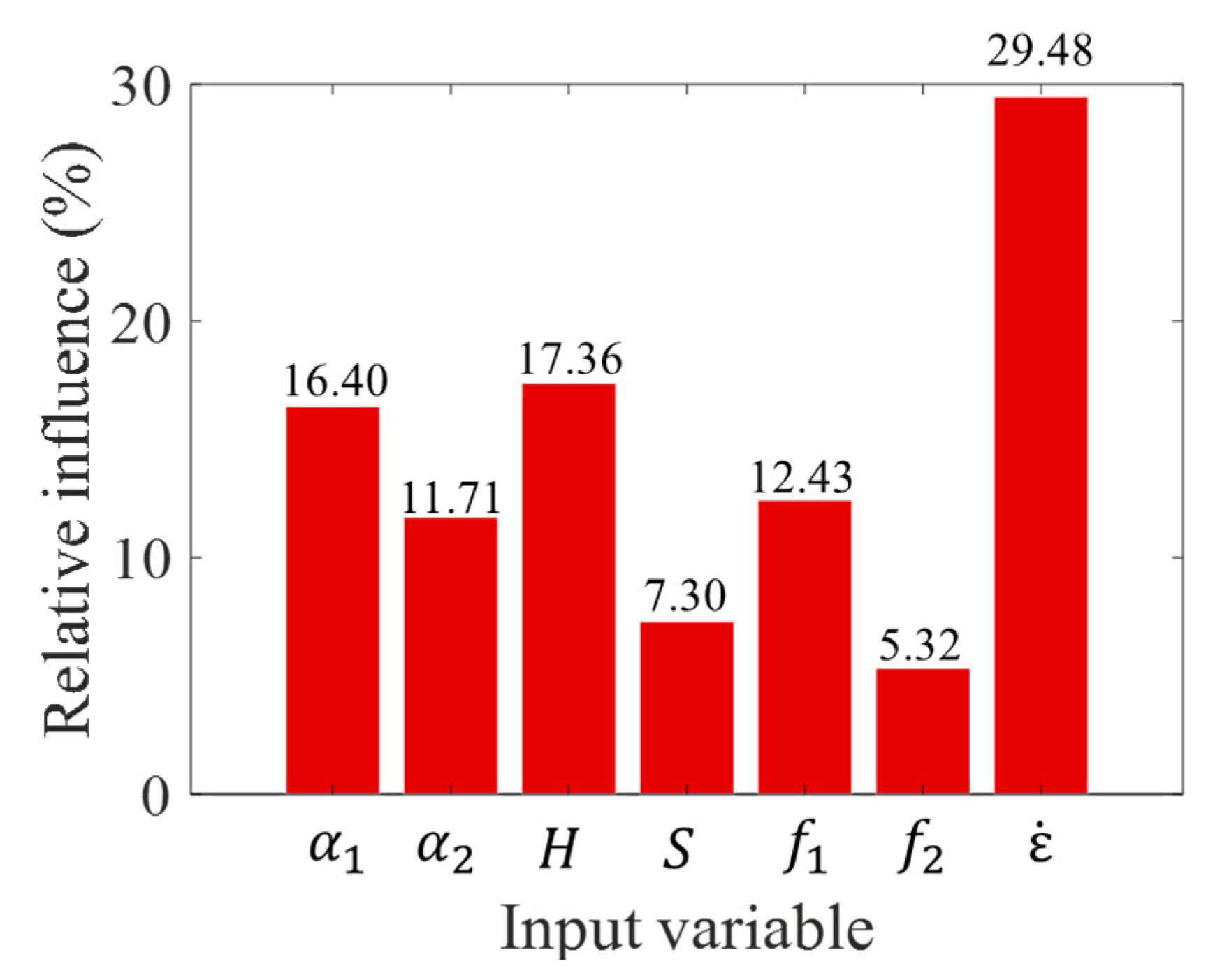
Figure 8 shows the relative influence of each individual input variable. The results of the analysis illustrate that the strength of heterogeneous rock is greatly affected by all considered input variables, while the strain rate ε ˙ is the most predominant variable affecting the rock strength in this study.
The effects of input number are further evaluated by comparing the mean absolute relative error derived from the entire dataset. The results for different selections of inputs are summarized in Table 4. Note that all ANN models with different inputs are trained under the same ANN setting listed in Table 2. It can be observed from Table 2 that the reduction in the inputs will decrease the overall performance of the ANN models in the current study. In particular, the strain rate ε ˙ cannot be ignored here because of the large prediction error presented in Case 8, which also validates the sensitivity analysis results. The error difference among other reported cases is, to some extent, not obvious.

4. Conclusions

The present study shows that the artificial neural network (ANN) approach can be applied to predict the influences of heterogeneity on rock strength at different strain rates. In the current study, seven input variables (initial crack inclination angle α 1 , α 2 ; relative position H , S ; filling material f 1 , f 2 and strain rate ε ˙ ) are considered and only one output variable, peak load P L . The best prediction performance of the ANN is observed when using the tan-sigmoid transfer functions in both the hidden and output layers, as well as the five neurons contained in the single hidden layer. Although only a limited number of experiment tests are implemented, the trained ANN presents a fast and accurate strength predicting performance, as reflected in the overall regression value of 0.9951. Finally, the sensitivity study for the input variables determines that strain rate is the most important factor affecting the mechanical performance of heterogeneous rocks. In the practical application process, the rock strength can be forecasted by several simple and measurable physical variables. In conclusion, the strong capacity for rapid convergence and high predictive accuracy of the ANN model is corroborated.
Limited by current experimental tests, the input variable pairs, namely α 1 , α 2 and f 1 , f 2 , both have the same values. Therefore, the applicability of the trained ANN model for more complex conditions concerning flaws with diverse crack inclination angles and filling material needs to be further validated by corresponding experiments. Because the ANN approach has the inherent advantage of being able to be extended (in terms of both depth and width), it possesses promising potential for establishing a more complex nonlinear relationship between the rock strength and rock heterogeneity when more heterogeneous physical quantities are involved. However, from a practice point of view, further systematic sampling with variations poses a great challenge for the large quantity of high-quality laboratory-tested samples, which may be problematic for some special fragile or heavily weathered rocks, as mentioned above. Hence, the proposed ANN approach, to some extent, can minimize the number of unnecessary experiments in order to ensure the rapid estimation of rock mechanical properties, which provides an alternative means of handling complex rock engineering problems. At the same time, with the aid of the more complete database, the reliability of the proposed ANN model can be further validated. It is worth noting that the current ANN approach cannot provide detailed information on failure patterns, such as those in experiments and simulations, and further research is deemed necessary.

Author Contributions

Conceptualization, S.J. and L.S.; Data curation, M.S.; Funding acquisition, L.S.; Investigation, S.J. and M.S.; Methodology, S.J.; Project administration, L.S.; Supervision, L.S.; Validation, S.J.; Writing—original draft, S.J.; Writing—review & editing, M.S. and L.S. All authors have read and agreed to the published version of the manuscript.

Funding

The work was supported in part by the Australian Research Council through Discovery Projects (DP190102954 and DP200101919). The authors acknowledge the use of the National Computational Infrastructure (NCI), which is supported by the Australian Government, and accessed through the Sydney Informatics Hub HPC Allocation Scheme, which is supported by the Deputy Vice-Chancellor (Research), University of Sydney and the ARC LIEF, 2019: Smith, Muller, Thornber et al., Sustaining and strengthening merit-based access to National Computational Infrastructure (LE190100021).

Institutional Review Board Statement

Not applicable.

Informed Consent Statement

Not applicable.

Data Availability Statement

The data presented in this study are available on request from the corresponding author.

Conflicts of Interest

The authors declare no conflict of interest. The funders had no role in the design of the study; in the collection, analyses, or interpretation of data; in the writing of the manuscript, or in the decision to publish the results.

Appendix A

Table A1. Summarization of the experimental raw dataset prepared for ANN and trained ANN predicted results.
Test No.InputOutput
Initial Crack Inclination Angle from Loading Axis (o)Relative Position (mm)FillingStrain Rate (s−1)Peak Load (N)
ExperimentANN
α 1 α 2 H S f 1 f 2 ε ˙ P L PL
1909000000.000115151486.098
2757500000.000113331326.732
3606000000.000113061225.101
4454500000.00019561196.695
5303000000.000111091204.291
6151500000.000111691238.981
70000000.000113801319.490
8909000110.000116781725.743
9757500110.000115331523.316
10606000110.000114761444.671
11454500110.000113691445.347
12303000110.000115201494.781
13151500110.000115571610.455
140000110.000118431849.571
15909007.334000.000114231443.698
16757507.334000.000117561305.584
17606007.334000.000112301195.725
18454507.334000.000111051159.104
19303007.334000.000111011164.367
20151507.334000.000111691200.831
210007.334000.000112171288.699
22909007.334110.000118161643.400
23757507.334110.000120491453.946
24606007.334110.000113651367.216
25454507.334110.000111711368.303
26303007.334110.000113541428.184
27151507.334110.000118321568.657
280007.334110.000118561855.662
2990905.5555.686000.000113591377.247
3075755.5555.686000.000115221346.187
3160605.5555.686000.000112701262.478
3245455.5555.686000.00018191154.207
3330305.5555.686000.00018941096.502
3415155.5555.686000.000110021083.879
35005.5555.686000.000111401093.918
3690905.5555.686110.000116201665.344
3775755.5555.686110.000117321623.381
3860605.5555.686110.000115541489.184
3945455.5555.686110.000112561379.604
4030305.5555.686110.000114191366.166
4115155.5555.686110.000114561417.751
42005.5555.686110.000115181526.933
439090000035036503663.233
447575000035037003617.357
456060000035036303620.612
464545000035036553639.233
473030000035036703658.648
481515000035036973677.001
4900000035036753695.113
509090001135040103925.057
517575001135039803916.149
526060001135039303929.861
534545001135039003949.114
543030001135039453969.769
551515001135039553991.496
5600001135039504014.363
57909007.3340035036503724.057
58757507.3340035038103665.866
59606007.3340035037683679.004
60454507.3340035037953726.472
61303007.3340035038253781.462
62151507.3340035038503836.380
630007.3340035038053889.384
64909007.3341135043004268.950
65757507.3341135043504270.513
66606007.3341135040054279.144
67454507.3341135043654288.077
68303007.3341135043864295.510
69151507.3341135043704301.435
700007.3341135043904306.144
7190905.5555.6860035034103400.248
7275755.5555.6860035035503521.862
7360605.5555.6860035035103487.539
7445455.5555.6860035035003492.108
7530305.5555.6860035035203547.000
7615155.5555.6860035034803610.143
77005.5555.6860035034753667.492
7890905.5555.6861135039304020.174
7975755.5555.6861135039753946.840
8060605.5555.6861135039103964.291
8145455.5555.6861135039703980.738
8230305.5555.6861135039553982.104
8315155.5555.6861135039803936.657
84005.5555.6861135040103932.417

References

  1. Jiang, S.; Shen, L.; Guillard, F.; Einav, I. Energy dissipation from two-glass-bead chains under impact. Int. J. Impact Eng. 2018, 114, 160–168. [Google Scholar] [CrossRef]
  2. Jiang, S.; Shen, L.; Guillard, F.; Einav, I. The effect of inter-grain contact material on the dynamic fracture of short glass bead chains under impact. Powder Technol. 2018, 339, 911–921. [Google Scholar] [CrossRef]
  3. Zhao, Y.; Zhang, L.; Wang, W.; Pu, C.; Wan, W.; Tang, J. Cracking and stress–strain behavior of rock-like material containing two flaws under uniaxial compression. Rock Mech. Rock Eng. 2016, 49, 2665–2687. [Google Scholar] [CrossRef]
  4. Fan, X.; Li, K.; Lai, H.; Xie, Y.; Cao, R.; Zheng, J. Internal stress distribution and cracking around flaws and openings of rock block under uniaxial compression: A particle mechanics approach. Comput. Geotech. 2018, 102, 28–38. [Google Scholar] [CrossRef]
  5. Wong, R.H.C.; Chau, K.T.; Tang, C.A.; Lin, P. Analysis of crack coalescence in rock-like materials containing three flaws—part I: Experimental approach. Int. J. Rock Mech. Min. Sci. 2001, 38, 909–924. [Google Scholar] [CrossRef]
  6. Tang, C.A.; Lin, P.; Wong, R.H.C.; Chau, K.T. Analysis of crack coalescence in rock-like materials containing three flaws—part II: Numerical approach. Int. J. Rock Mech. Min. Sci. 2001, 38, 925–939. [Google Scholar] [CrossRef]
  7. Nicholson, D.T.; Nicholson, F.H. Physical deterioration of sedimentary rocks subjected to experimental freeze–thaw weathering. Earth Surf. Process. Landf. J. Br. Geomorphol. Res. Group 2000, 25, 1295–1307. [Google Scholar] [CrossRef]
  8. Le, H.; Sun, S.; Kulatilake, P.H.; Wei, J. Effect of grout on mechanical properties and cracking behavior of rock-like specimens containing a single flaw under uniaxial compression. Int. J. Geomech. 2018, 18, 04018129. [Google Scholar] [CrossRef]
  9. Duan, L.; Zhang, Y.; Lai, J. Influence of ground temperature on shotcrete-to-rock adhesion in tunnels. Adv. Mater. Sci. Eng. 2019, 2019, 8709087. [Google Scholar] [CrossRef] [Green Version]
  10. Sharafisafa, M.; Aliabadian, Z.; Shen, L. Crack initiation and failure development in bimrocks using digital image correlation under dynamic load. Theor. Appl. Fract. Mech. 2020, 109, 102688. [Google Scholar] [CrossRef]
  11. Wang, Y.; Zhang, H.; Lin, H.; Zhao, Y.; Li, X.; Liu, Y. Mechanical behavior and failure analysis of fracture-filled gneissic granite. Theor. Appl. Fract. Mech. 2020, 108, 102674. [Google Scholar] [CrossRef]
  12. Liu, L.; Li, H.; Li, X.; Wu, D.; Zhang, G. Underlying mechanisms of crack initiation for granitic rocks containing a single pre-existing flaw: Insights from digital image correlation (DIC) analysis. Rock Mech. Rock Eng. 2020, 54, 1–17. [Google Scholar]
  13. Yan, Z.; Dai, F.; Liu, Y.; Du, H.; Luo, J. Dynamic Strength and Cracking Behaviors of Single-Flawed Rock Subjected to Coupled Static–Dynamic Compression. Rock Mech. Rock Eng. 2020, 53, 4289–4298. [Google Scholar] [CrossRef]
  14. Zhao, C.; Meng Zhou, Y.; Feng Zhao, C.; Bao, C. Cracking processes and coalescence modes in rock-like specimens with two parallel pre-existing cracks. Rock Mech. Rock Eng. 2018, 51, 3377–3393. [Google Scholar] [CrossRef]
  15. Huang, Y.-H.; Yang, S.-Q.; Tian, W.-L. Crack coalescence behavior of sandstone specimen containing two pre-existing flaws under different confining pressures. Theor. Appl. Fract. Mech. 2019, 99, 118–130. [Google Scholar] [CrossRef]
  16. Zhou, X.-P.; Li, G.-Q.; Ma, H.-C. Real-time experiment investigations on the coupled thermomechanical and cracking behaviors in granite containing three pre-existing fissures. Eng. Fract. Mech. 2020, 224, 106797. [Google Scholar] [CrossRef]
  17. Chen, S.; Xia, Z.; Feng, F.; Yin, D. Numerical study on strength and failure characteristics of rock samples with different hole defects. Bull. Eng. Geol. Environ. 2020, 80, 1–18. [Google Scholar] [CrossRef]
  18. Xi, X.; Wu, X.; Guo, Q.; Cai, M. Experimental investigation and numerical simulation on the crack initiation and propagation of rock with pre-existing cracks. IEEE Access 2020, 8, 129636–129644. [Google Scholar] [CrossRef]
  19. Wang, Y.; Zhang, H.; Lin, H.; Zhao, Y.; Liu, Y. Fracture behaviour of central-flawed rock plate under uniaxial compression. Theor. Appl. Fract. Mech. 2020, 106, 102503. [Google Scholar] [CrossRef]
  20. Liu, G.; Peng, J.; Zhang, Z.; Wang, Z.; Yang, Y. Numerical investigation of fluid-driven crack propagation and coalescence in granite specimen with two pre-existing flaws. J. Nat. Gas Sci. Eng. 2020, 75, 103132. [Google Scholar] [CrossRef]
  21. Shen, H.; Li, X.; Li, Q.; Wang, H. A method to model the effect of pre-existing cracks on P-wave velocity in rocks. J. Rock Mech. Geotech. Eng. 2020, 12, 493–506. [Google Scholar] [CrossRef]
  22. Altindag, R. Correlation between P-wave velocity and some mechanical properties for sedimentary rocks. J. South. Afr. Inst. Min. Metall. 2012, 112, 229–237. [Google Scholar]
  23. Liu, X.; Athanasiou, C.E.; Padture, N.P.; Sheldon, B.W.; Gao, H. A machine learning approach to fracture mechanics problems. Acta Mater. 2020, 190, 105–112. [Google Scholar] [CrossRef]
  24. Nasiri, S.; Khosravani, M.R.; Weinberg, K. Fracture mechanics and mechanical fault detection by artificial intelligence methods: A review. Eng. Fail. Anal. 2017, 81, 270–293. [Google Scholar] [CrossRef]
  25. Ziolkowski, P.; Niedostatkiewicz, M.; Kang, S.-B. Model-Based Adaptive Machine Learning Approach in Concrete Mix Design. Materials 2021, 14, 1661. [Google Scholar] [CrossRef] [PubMed]
  26. Atici, U. Prediction of the strength of mineral admixture concrete using multivariable regression analysis and an artificial neural network. Expert Syst. Appl. 2011, 38, 9609–9618. [Google Scholar] [CrossRef]
  27. Gope, D.; Gope, P.C.; Thakur, A.; Yadav, A. Application of artificial neural network for predicting crack growth direction in multiple cracks geometry. Appl. Soft Comput. 2015, 30, 514–528. [Google Scholar] [CrossRef]
  28. Yan, Y.; Ren, Q.; Xia, N.; Shen, L.; Gu, J. Artificial neural network approach to predict the fracture parameters of the size effect model for concrete. Fatigue Fract. Eng. Mater. Struct. 2015, 38, 1347–1358. [Google Scholar] [CrossRef]
  29. Mahmoodzadeh, A.; Mohammadi, M.; Ibrahim, H.H.; Abdulhamid, S.N.; Salim, S.G.; Ali, H.F.H.; Majeed, M.K. Artificial intelligence forecasting models of uniaxial compressive strength. Transp. Geotech. 2021, 27, 100499. [Google Scholar] [CrossRef]
  30. Ferentinou, M.; Fakir, M. An ANN approach for the prediction of uniaxial compressive strength, of some sedimentary and igneous rocks in eastern KwaZulu-Natal. Procedia Eng. 2017, 191, 1117–1125. [Google Scholar] [CrossRef]
  31. Sharafisafa, M.; Shen, L. Experimental Investigation of Dynamic Fracture Patterns of 3D Printed Rock-like Material Under Impact with Digital Image Correlation. Rock Mech. Rock Eng. 2020, 53, 1–19. [Google Scholar] [CrossRef]
  32. Sharafisafa, M.; Shen, L.; Zheng, Y.; Xiao, J. The effect of flaw filling material on the compressive behaviour of 3D printed rock-like discs. Int. J. Rock Mech. Min. Sci. 2019, 117, 105–117. [Google Scholar] [CrossRef]
  33. Sharafisafa, M.; Shen, L.; Xu, Q. Characterisation of mechanical behaviour of 3D printed rock-like material with digital image correlation. Int. J. Rock Mech. Min. Sci. 2018, 112, 122–138. [Google Scholar] [CrossRef]
  34. Mazahery, A.; Shabani, M.O. Process conditions optimization in Al–Cu alloy matrix composites. Powder Technol. 2012, 225, 101–106. [Google Scholar] [CrossRef]
  35. Levenberg, K. A method for the solution of certain non-linear problems in least squares. Q. Appl. Math. 1944, 2, 164–168. [Google Scholar] [CrossRef] [Green Version]
  36. Marquardt, D.W. An algorithm for least-squares estimation of nonlinear parameters. J. Soc. Ind. Appl. Math. 1963, 11, 431–441. [Google Scholar] [CrossRef]
  37. Naderpour, H.; Poursaeidi, O.; Ahmadi, M. Shear resistance prediction of concrete beams reinforced by FRP bars using artificial neural networks. Measurement 2018, 126, 299–308. [Google Scholar] [CrossRef]
  38. Faisal, A.A.; Naji, L.A. Simulation of ammonia nitrogen removal from simulated wastewater by sorption onto waste foundry sand using artificial neural network. Assoc. Arab Univ. J. Eng. Sci. 2019, 26, 28–34. [Google Scholar] [CrossRef]
  39. Garson, G.D. Interpreting neural-network connection weights. AI EXPERT 1991, 6, 47–51. [Google Scholar]
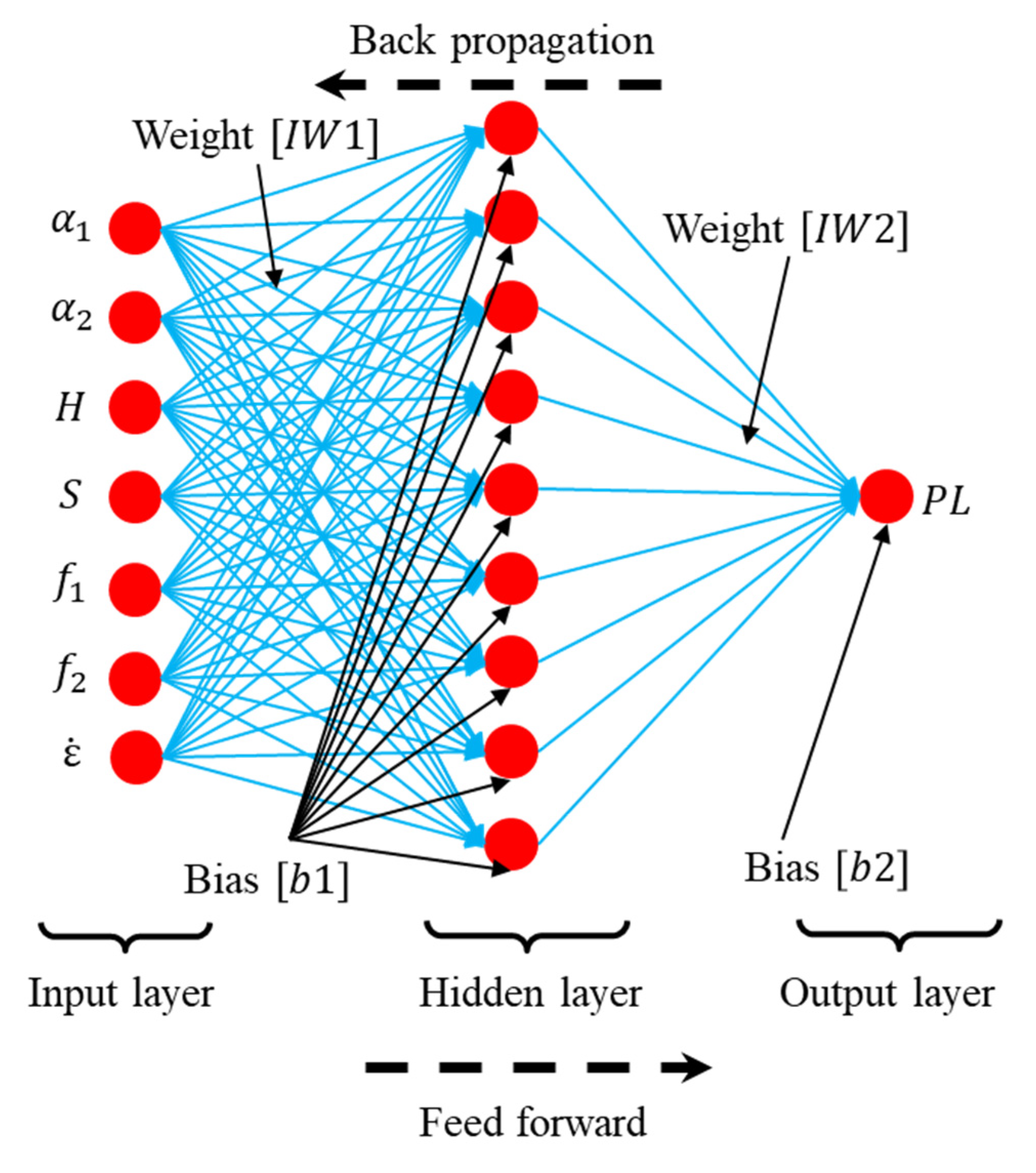
Figure 1. The architecture of an artificial neural network containing a single hidden layer.
Materials 14 03042 g001
Figure 2. (a) The schematic of an overlapped flaw configuration with input variables labeled; (b) the output (peak load) is extracted from a typical force–displacement curve.
Materials 14 03042 g002
Figure 3. The performances of ANNs with different transfer functions and normalization settings.
Materials 14 03042 g003
Figure 4. Performance of ANNs with different hidden neuron numbers.
Materials 14 03042 g004
Figure 5. The typical training process of ANN.
Materials 14 03042 g005
Figure 6. The regression values of the trained ANN.
Materials 14 03042 g006
Figure 7. (a) The comparison of predicted and experimental results; (b) the corresponding relative error for each test.
Materials 14 03042 g007
Figure 8. The sensitivity importance of input variables.
Materials 14 03042 g008
Table 1. Combinations of different transfer functions and normalization settings.
Case No.Input VariablesHidden LayerOutput LayerOutput Variable
1NormalizedTan-sigmoidTan-sigmoidNormalized
2NormalizedTan-sigmoidSigmoidNormalized
3NormalizedSigmoidSigmoidNormalized
4NormalizedTan-sigmoidLinearRaw
5NormalizedSigmoidLinearRaw
6RawTan-sigmoidLinearRaw
7RawSigmoidLinearRaw
Table 2. The ANN setting for predicting peak load.
Input layer neuron number7
Hidden layer neuron number5
Output layer neuron number1
Data divisionRandomly (70% training, 15% validation, 15% testing)
Hidden layer transfer functionTan-sigmoid
Output layer transfer functionTan-sigmoid
Early stopping criterion10 epochs for validation check
Target error10−6
Training algorithmLevenberg–Marquardt
Table 3. Descriptive statistics of the peak loads predicted by the ANN approach.
Test No. P L A N N / P L E x p e r i m e n t Mean Absolute Relative Error (%)
MeanSDCOV (%)
Static (No.1–No.42)1.010.121.377.46
Dynamic (No.43–No.84)1.000.020.041.51
Overall (No.1–No.84)1.000.080.704.49
Table 4. Effects of input number on the prediction by ANN models.
Case No.Number of InputsInputsMean Absolute Relative Error (%)
17 α 1 , α 2 ,   H , S ,   f 1 , f 2 , ε ˙ 4.49 (Reference)
26 α 2 ,   H , S ,   f 1 , f 2 ,   ε ˙ 6.26
3 α 1 , H , S ,   f 1 , f 2 ,   ε ˙ 5.75
4 α 1 , α 2 , S ,   f 1 , f 2 ,   ε ˙ 7.39
5 α 1 , α 2 , H , f 1 , f 2 ,   ε ˙ 6.02
6 α 1 , α 2 , H , S ,   f 2 ,   ε ˙ 5.96
7 α 1 , α 2 , H , S ,   f 1 ,   ε ˙ 6.36
8 α 1 , α 2 , H , S ,   f 1 , f 2 68.40
95 α 1 , H ,   f 1 , f 2 ,   ε ˙ 6.38
10 α 1 ,   H , S ,   f 1 ,   ε ˙ 6.43
11 α 1 , α 2 , H , f 1 ,   ε ˙ 6.50
124 α 1 ,   H ,   f 1 ,   ε ˙ 6.10
Publisher’s Note: MDPI stays neutral with regard to jurisdictional claims in published maps and institutional affiliations.