
Optimization of Optical Machine Structure by Backpropagation Neural Network Based on Particle Swarm Optimization and Bayesian Regularization Algorithms


Abstract
:1. Introduction
2. Basic Theory
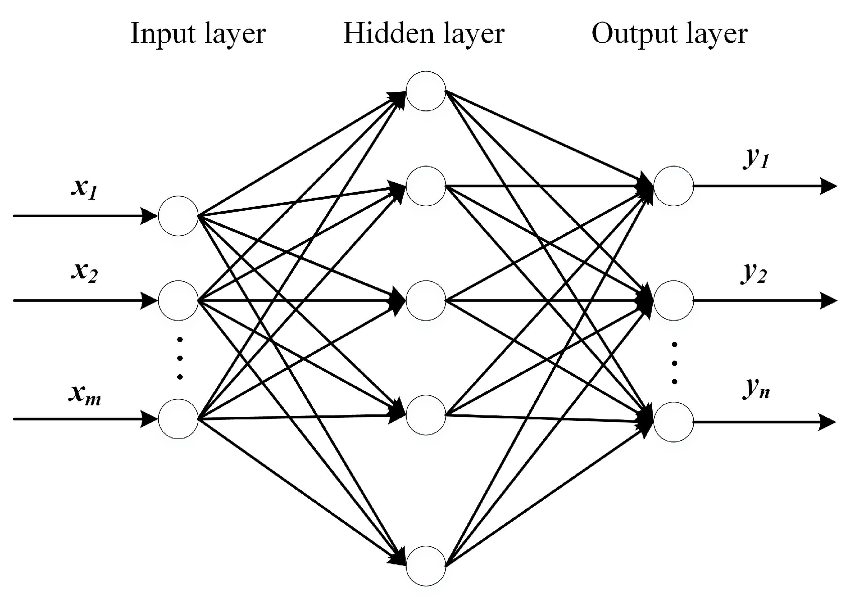
2.1. BPNN Method
2.2. PSO Algorithm
2.3. BR Algorithm
2.4. BMPB
3. Optimal Design Process of an Optical Machine Structure
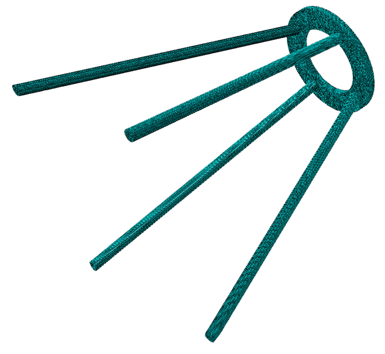
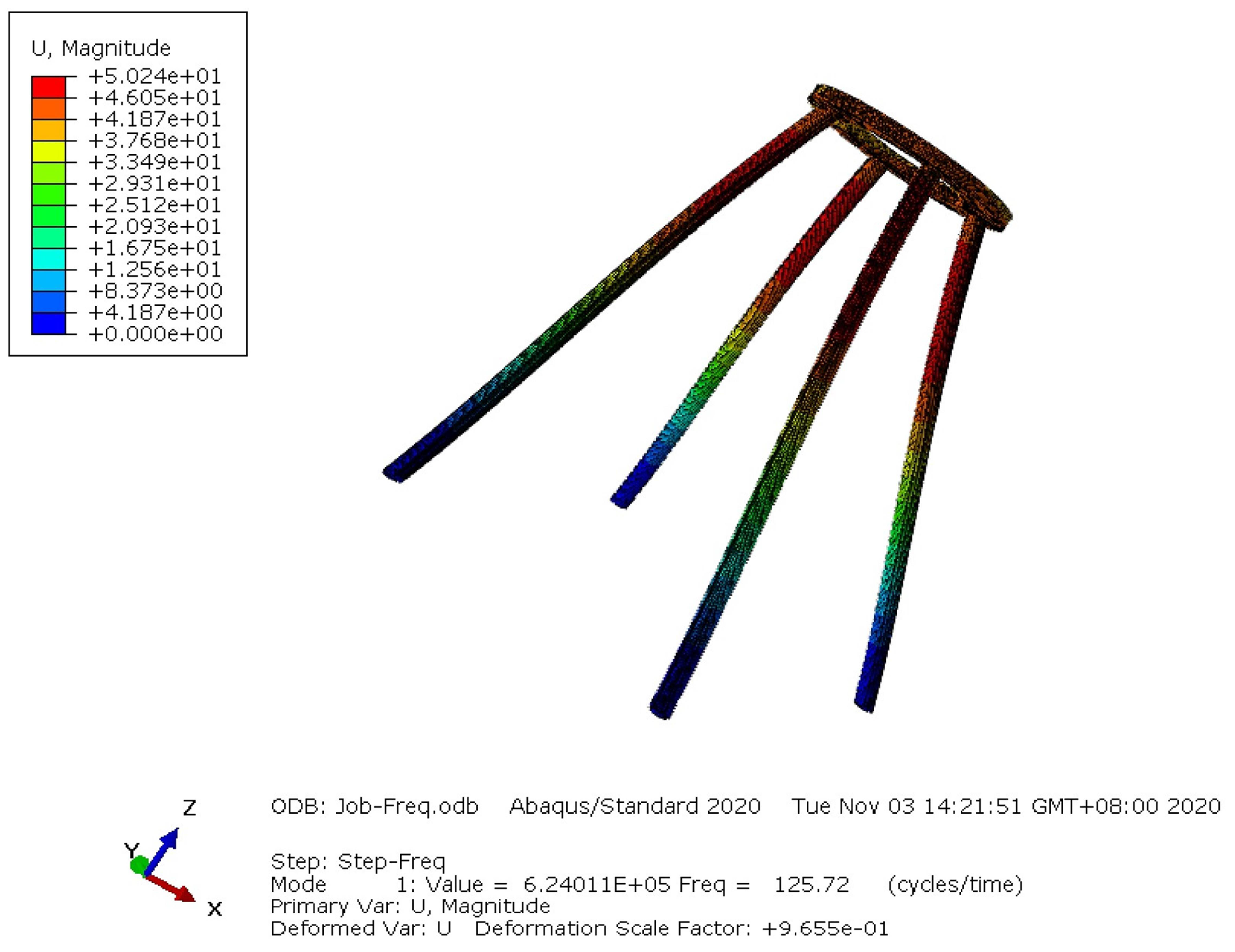
3.1. Finite Element Calculation and Integrated Analysis
3.2. Training Neural Network Model
3.3. Optimization of Optical Machine Structure Performance Index
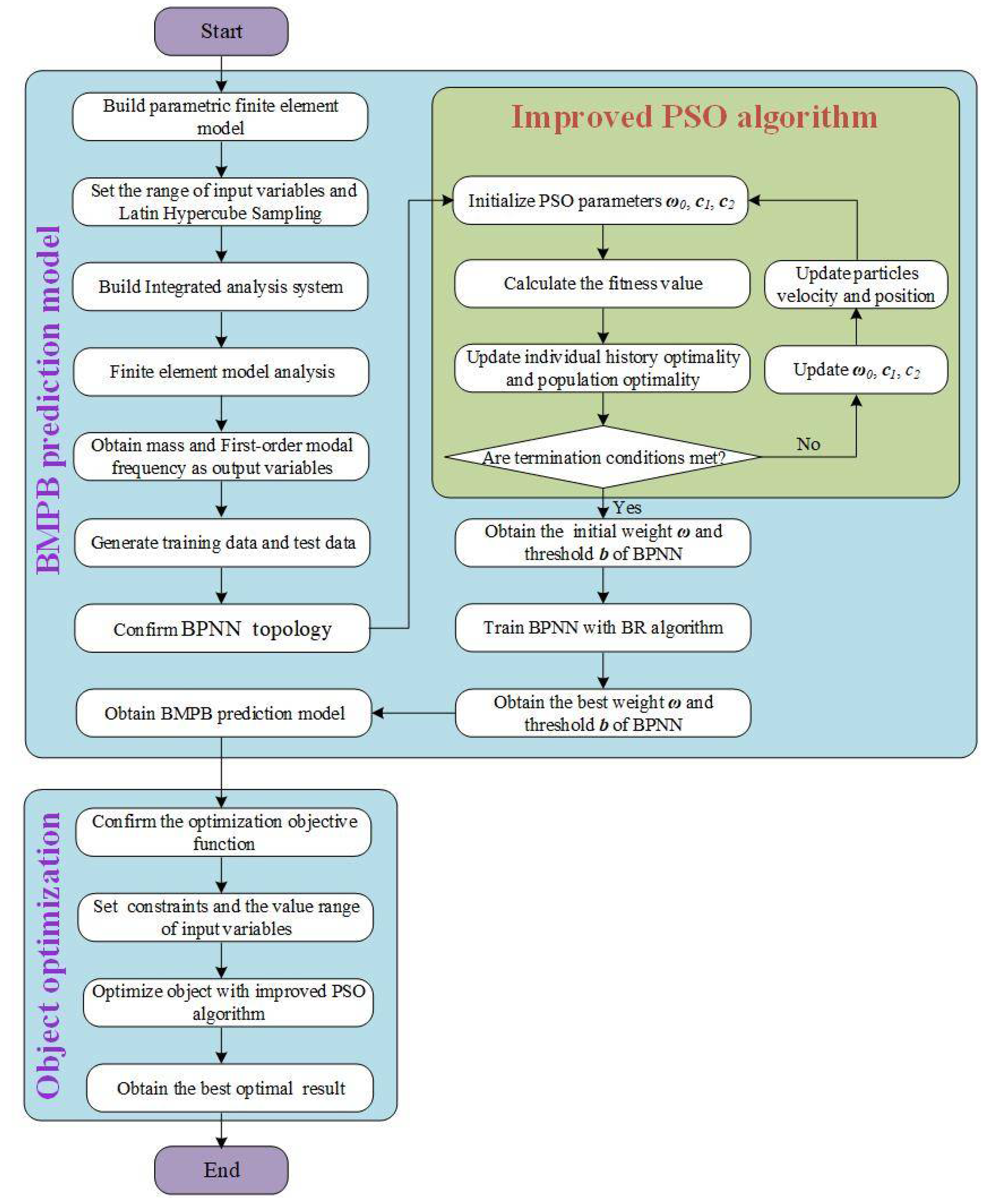
3.4. Optimization Flow Chart
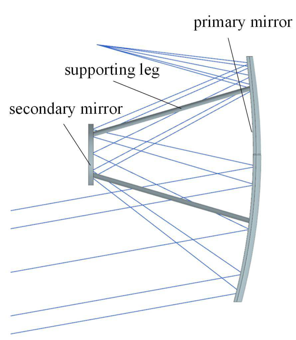
4. Optimal Design of Supporting Structure
4.1. Preliminary Preparation
4.2. Integrated Analysis
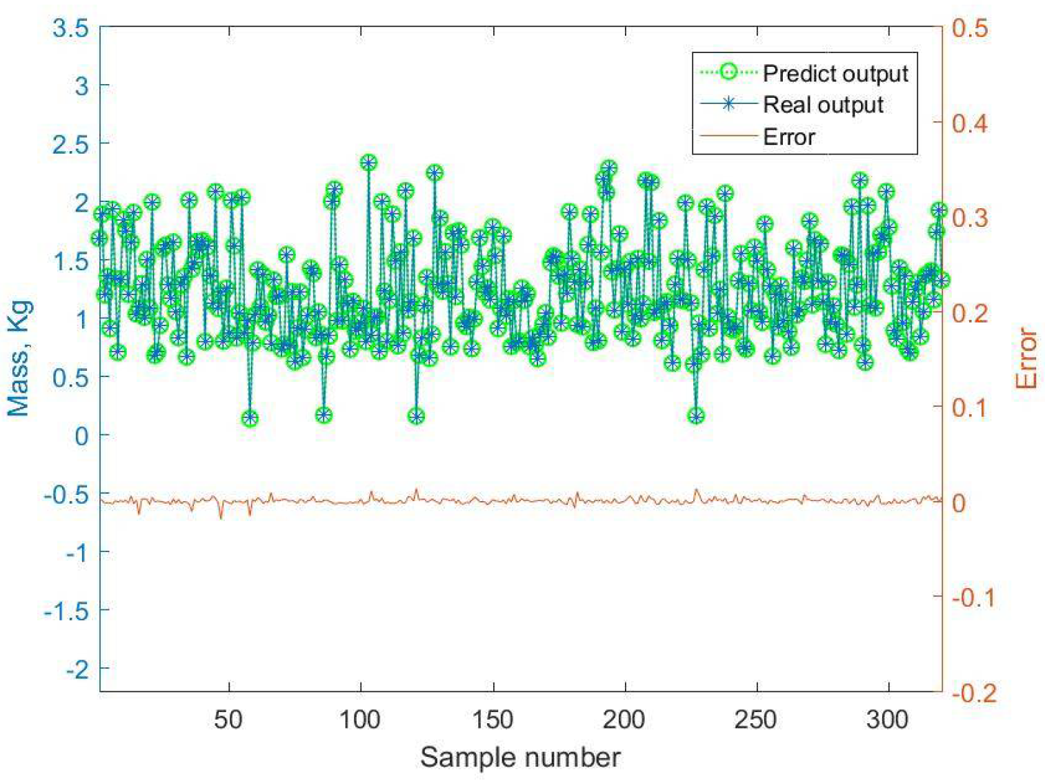
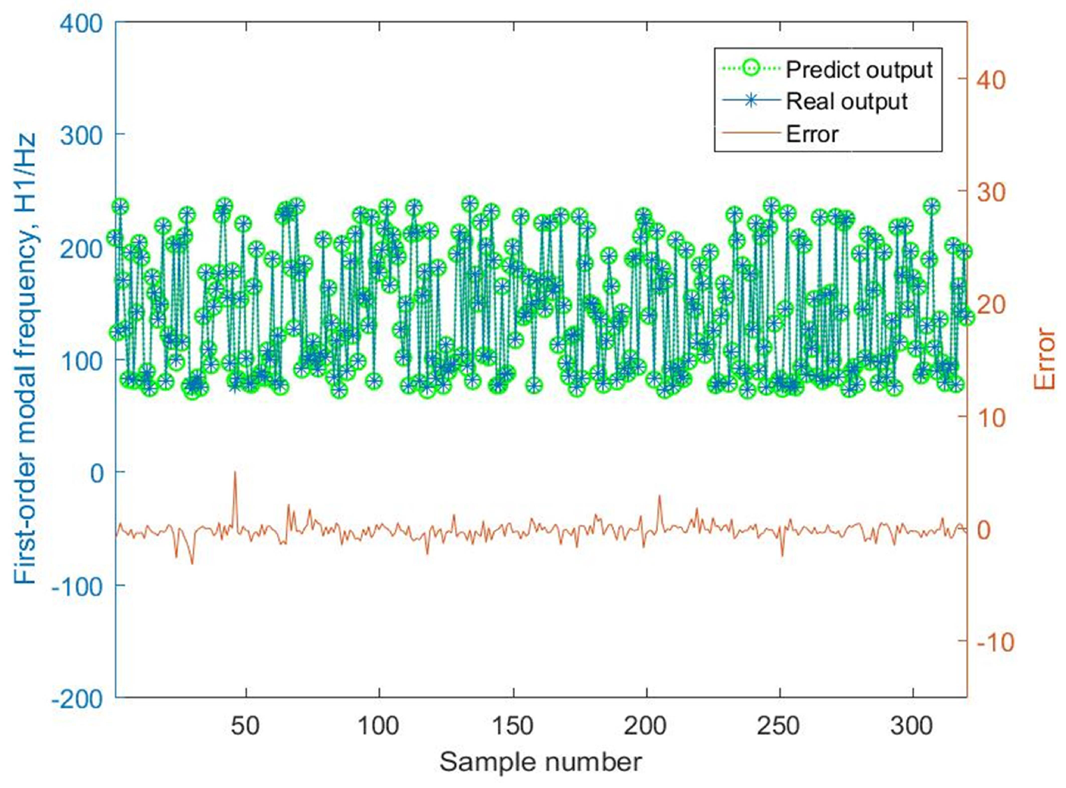
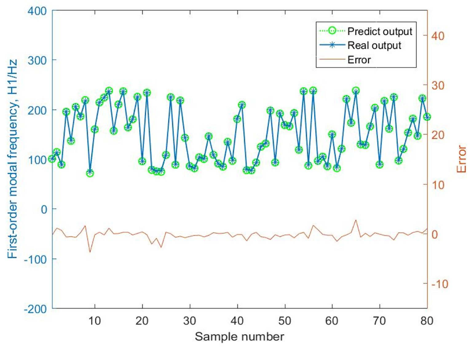
4.3. Build the BMPB Model
4.4. The Optimization of Supporting Structure Mass
4.5. Analysis
5. Conclusions
Author Contributions
Funding
Institutional Review Board Statement
Informed Consent Statement
Data Availability Statement
Conflicts of Interest
Abbreviations
| BMPB | backpropagation neural network method based on particle swarm optimization and Bayesian regularization algorithms |
| FEA | finite element analysis |
| MCM | Monte Carlo method |
| BPNN | backpropagation neural network |
| PSO | particle swarm optimization |
| BR | Bayesian regularization |
| BPGA | backpropagation neural network based on genetic algorithm |
References
- Wei, L.; Zhang, L.; Gong, X.; Ma, D.-M. Design and optimization for main support structure of a large-area off-axis three-mirror space camera. Appl. Opt. 2017, 56, 1094–1100. [Google Scholar] [CrossRef] [PubMed]
- Gan, X. Design for main support of long focal length space camera. In Proceedings of the 2011 International Conference on Mechatronic Science, Electric Engineering and Computer (MEC), Jilin, China, 19–22 August 2011; pp. 515–518. [Google Scholar]
- Zhu, C.; Xu, T.; Liu, S.; Bo, Y.; Liu, Y. Design of primary mirror supporting structure and lightweight of space camera. In Proceedings of the SPIE—The International Society for Optical Engineering, Xiamen, China, 26–29 April 2012; Volume 8416. [Google Scholar]
- Yu, F.; Xu, S. Support structure and optical alignment technology of large-aperture secondary mirror measured by back transmission method. Optik 2020, 207, 164274. [Google Scholar] [CrossRef]
- Xia, S.; Shi, J.; Ren, G.; Li, C. Calibration Mechanism Design and Stiffness Analysis. IOP Conf. Ser. Mater. Sci. Eng. 2019, 520, 012014. [Google Scholar] [CrossRef]
- Wu, J. Design of High-lightweight Space Mirror Component Based on Automatic Optimization. J. Phys. Conf. Ser. 2020, 1605, 012023. [Google Scholar] [CrossRef]
- Han, Y.-Y.; Zhang, Y.-M.; Han, J.-C.; Zhang, J.-H.; Yao, W.; Zhou, Y.-F. Design and finite element analysis of lightmass silicon carbide primary mirror. Trans. Nonferrous Met. Soc. China 2006, 16, 696–700. [Google Scholar] [CrossRef]
- Lin, Y.C.; Lee, L.J.; Chang, S.T.; Cheng, Y.C.; Huang, T.M. Numerical and Experimental Analysis of Light-Weighted Primary Mirror for Cassegrain Telescope. Appl. Mech. Mater. 2011, 52–54, 59–64. [Google Scholar] [CrossRef]
- Williamson, M.P. Finite-element analysis. Comput. Aided Eng. J. 1985, 2, 66–69. [Google Scholar] [CrossRef]
- Zhu, Y.; Zhang, Y.; Shi, J. Finite element analysis of flexural behavior of precast segmental UHPC beams with prestressed bolted hybrid joints. Eng. Struct. 2021, 238, 111492. [Google Scholar] [CrossRef]
- Meguid, S.A.; Kanth, P.S.; Czekanski, A. Finite element analysis of fir-tree region in turbine discs. Finite Elem. Anal. Des. 2000, 35, 305–317. [Google Scholar] [CrossRef]
- Tmr, A.; Dm, A.; Fab, C.; Oduj, A.; Jdc, A.; Bhj, D.; Dan, S.; Jam, A.; Jdm, A. Simulation of Powder Bed Metal Additive Manufacturing Microstructures with Coupled Finite Difference-Monte Carlo Method. Addit. Manuf. 2021, 41, 101953. [Google Scholar]
- Nakonechnyi, A.N.; Shpak, V.D. Adaptive optimization of the Monte-Carlo method. Cybern. Syst. Anal. 1994, 30, 34–40. [Google Scholar] [CrossRef]
- Yu, W.; Cao, Z.; Au, S.K. Efficient Monte Carlo Simulation of parameter sensitivity in probabilistic slope stability analysis. Comput. Geotech. 2010, 37, 1015–1022. [Google Scholar]
- Guggenberger, J.; Grundmann, H. Monte Carlo simulation of the hysteretic response of frame structures using plastification adapted shape functions. Probabilistic Eng. Mech. 2004, 19, 81–91. [Google Scholar] [CrossRef]
- Asri, Y.M.; Azrulhisham, E.A.; Dzuraidah, A.W.; Shahrir, A.; Shahrum, A.; Azami, Z. Fatigue life reliability prediction of a stub axle using Monte Carlo simulation. Int. J. Automot. Technol. 2011, 12, 713–719. [Google Scholar] [CrossRef]
- Song, L.-K.; Bai, G.-C.; Fei, C.W. Probabilistic LCF life assessment for turbine discs with DC strategy-based wavelet neural network regression. Int. J. Fatigue 2019, 119, 204–219. [Google Scholar] [CrossRef]
- Lks, A.; Cwfa, B.; Jie, W.A.; Gcb, A. Multi-objective reliability-based design optimization approach of complex structure with multi-failure modes—ScienceDirect. Aerosp. Sci. Technol. 2017, 64, 52–62. [Google Scholar]
- Wang, Z.; Zhang, J.A.; Wang, J.C.; He, X.A.; Fu, L.A.; Tian, F.A.; Liu, X.A.; Zhao, Y.A. A Back Propagation neural network based optimizing model of space-based large mirror structure. Optik 2019, 179, 780–786. [Google Scholar] [CrossRef]
- Wang, D.; Zhang, S.; Tan, F.; Zhi, X.; Zhen, R. A method on lightweight for the primary mirror of large space-based telescope based on neural network. In Proceedings of the International Symposium on Optoelectronic Technology & Application: Imaging Spectroscopy & Telescopes & Large Optics, Beijing, China, 13–15 May 2014. [Google Scholar]
- Charytoniuk, W.; Chen, M.S. Short-term load forecasting using Artificial Neural Networks. A review and evaluation. IEEE Trans. Power Syst. 2000, 15, 263–268. [Google Scholar] [CrossRef]
- Magalhaes, F.C.; Ventura, C.; Abrao, A.M.; Denkena, B.; Meyer, K. Prediction of surface residual stress and hardness induced by ball burnishing through neural networks. Int. J. Manuf. Res. 2019, 14, 295–310. [Google Scholar] [CrossRef]
- Jung, Y.W.; Kim, H.K. Prediction of Nonlinear Stiffness of Automotive Bushings by Artificial Neural Network Models Trained by Data from Finite Element Analysis. Int. J. Automot. Technol. 2020, 21, 1539–1551. [Google Scholar] [CrossRef]
- Al-Garni, A.Z.; Jamal, A.; Ahmad, A.M.; Al-Garni, A.M.; Tozan, M. Neural network-based failure rate prediction for De Havilland Dash-8 tires. Eng. Appl. Artif. Intell. 2006, 19, 681–691. [Google Scholar] [CrossRef]
- Panagiotis, A.; Panayiotis, R.; Maria, D. Feed-Forward Neural Network Prediction of the Mechanical Properties of Sandcrete Materials. Sensors 2017, 17, 1344. [Google Scholar]
- Zhao, Q.; Liu, Q.; Cao, N.; Guan, F.; Wang, H. Stepped generalized predictive control of test tank temperature based on backpropagation neural network. AEJ Alex. Eng. J. 2020, 60, 357–364. [Google Scholar] [CrossRef]
- Feng, G.; Lei, S.; Gu, X.; Guo, Y.; Wang, J. Predictive control model for variable air volume terminal valve opening based on backpropagation neural network—ScienceDirect. Build. Environ. 2021, 188, 107485. [Google Scholar] [CrossRef]
- Jin, C.; Jin, S.W.; Qin, L.N. Attribute selection method based on a hybrid BPNN and PSO algorithms. Appl. Soft Comput. 2012, 12, 2147–2155. [Google Scholar] [CrossRef]
- Kennedy, J. Particle swarm optimization. In Proceedings of the ICNN’95—International Conference on Neural Networks, Perth, WA, Australia, 27 November–1 December 1995; Volume 4, pp. 1942–1948. [Google Scholar]
- Gomes, H.M. Truss optimization with dynamic constraints using a particle swarm algorithm. Expert Syst. Appl. 2011, 38, 957–968. [Google Scholar] [CrossRef]
- Xu, L.; Huang, C.; Li, C.; Wang, J.; Wang, X. Estimation of tool wear and optimization of cutting parameters based on novel ANFIS-PSO method toward intelligent machining. J. Intell. Manuf. 2021, 32, 77–90. [Google Scholar] [CrossRef]
- Cawley, G.C.; Talbot, N. Preventing Over-Fitting during Model Selection via Bayesian Regularisation of the Hyper-Parameters. J. Mach. Learn. Res. 2007, 8, 841–861. [Google Scholar]


| Random Variables | Max, m | Min, m |
|---|---|---|
| 0.03 | 0.010 | |
| 0.006 | 0.002 |
| Evaluation Indicators | MAE, kg | MSE, kg2 | RMSE, kg | MPA |
|---|---|---|---|---|
| Training samples | 2.2127 × 10⁻³ | 1.0489 × 10⁻⁵ | 3.2387 × 10⁻³ | 99.73% |
| Test samples | 2.1471 × 10⁻³ | 1.0429 × 10⁻⁵ | 3.2293 × 10⁻³ | 99.81% |
| Evaluation Indicators | MAE, Hz | MSE, Hz2 | RMSE, Hz | MPA |
|---|---|---|---|---|
| Training samples | 0.5368 | 0.5943 | 0.7709 | 99.55% |
| Test samples | 0.6078 | 0.8135 | 0.9019 | 99.49% |
| Mass | ||
|---|---|---|
| 0.0168 m | 0.002 m | 0.7422 kg |
| Method | Optimization Time | Optimization Result | Accuracy |
|---|---|---|---|
| MCM | 1.04 × 10⁵ s | 0.7532 kg | 100% |
| BPGA | 476 s | 0.8850 kg | 91.4% |
| BMPB | 56 s | 0.7422 kg | 99.4% |
Publisher’s Note: MDPI stays neutral with regard to jurisdictional claims in published maps and institutional affiliations. |
© 2021 by the authors. Licensee MDPI, Basel, Switzerland. This article is an open access article distributed under the terms and conditions of the Creative Commons Attribution (CC BY) license (https://creativecommons.org/licenses/by/4.0/).
Share and Cite
Zhang, X.; Sun, L. Optimization of Optical Machine Structure by Backpropagation Neural Network Based on Particle Swarm Optimization and Bayesian Regularization Algorithms. Materials 2021, 14, 2998. https://doi.org/10.3390/ma14112998
Zhang X, Sun L. Optimization of Optical Machine Structure by Backpropagation Neural Network Based on Particle Swarm Optimization and Bayesian Regularization Algorithms. Materials. 2021; 14(11):2998. https://doi.org/10.3390/ma14112998
Chicago/Turabian StyleZhang, Xinyong, and Liwei Sun. 2021. "Optimization of Optical Machine Structure by Backpropagation Neural Network Based on Particle Swarm Optimization and Bayesian Regularization Algorithms" Materials 14, no. 11: 2998. https://doi.org/10.3390/ma14112998
APA StyleZhang, X., & Sun, L. (2021). Optimization of Optical Machine Structure by Backpropagation Neural Network Based on Particle Swarm Optimization and Bayesian Regularization Algorithms. Materials, 14(11), 2998. https://doi.org/10.3390/ma14112998