A Novel Approach to Describe the Time–Temperature Conversion among Relaxation Curves of Viscoelastic Materials

 ,
,  ,
,  and
and
Abstract
1. Introduction
2. The Current Methodology
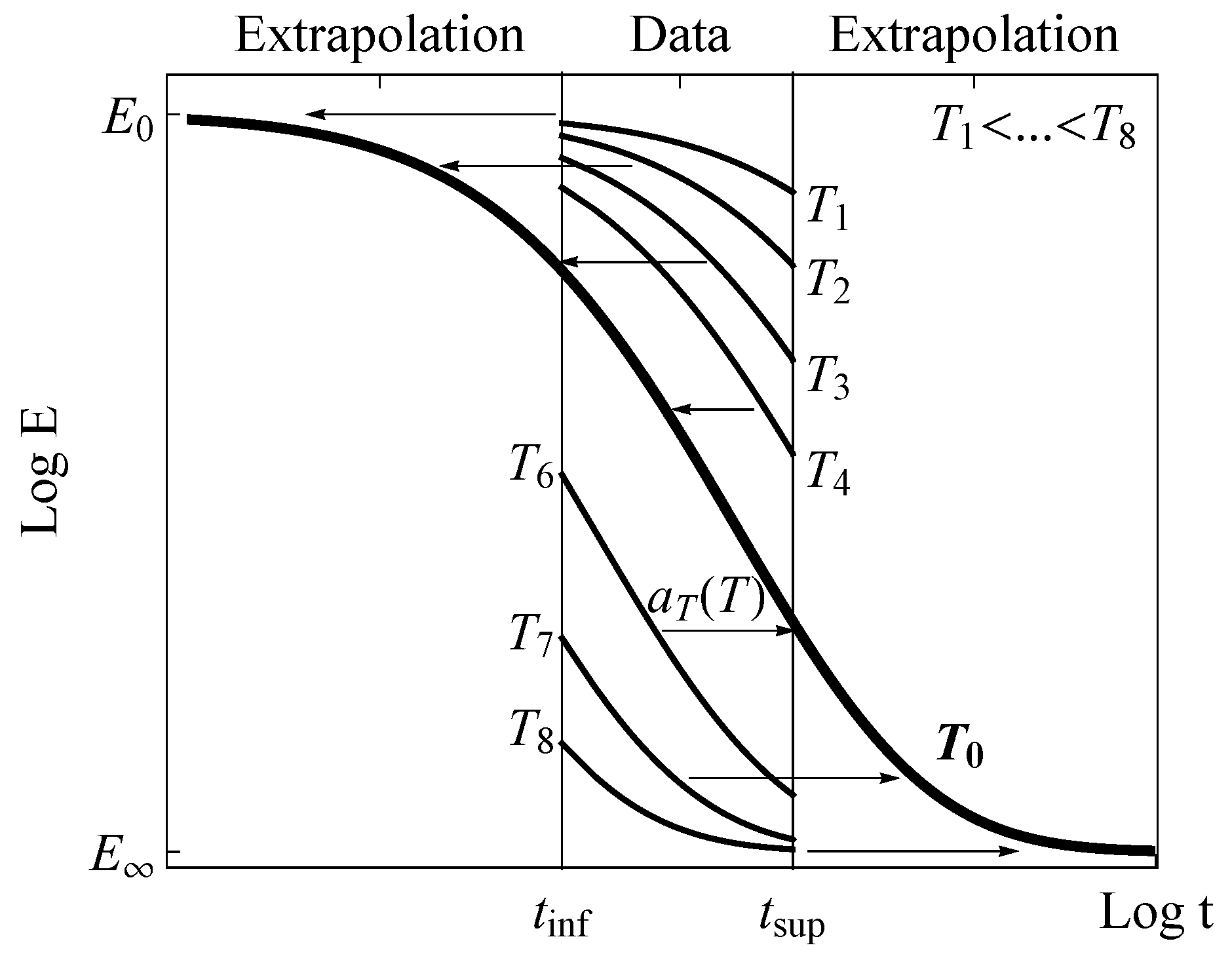
- Derivation of the master curve. The first step consists in deriving the master curve from the experimental data (see Figure 1) by shifting the relaxation curves in the horizontal direction according to the law briefly described in the previous section.
- Estimation of the experimental shift factors . In the second step, a first approximation of the master curve is achieved, traditionally using manual estimative shifting of the relaxation curves. Thereby, shift factors are chosen, which because their arbitrary selection may lead to notably different solutions of the final master curve or even of the TTS model as a whole. Fortunately, in recent years, some new algorithms, such as the CFS algorithm developed by Gergesova et al. [7], allow such a manual shifting to be overcome thus enhancing considerably the accuracy in the derivation of the master curve. The method requires a minimum overlapping among the registered fragments of the relaxation curves to be applied.This step 2 implies the analysis of the experimental shift factors before fitting the TTS model. One of the main problems is that in general, different trends for the shift factors are noticed depending on them being determined below or above the glass transition temperature (see Tanaka [8] and Ferry [2]). Therefore, more than one TTS model is sometimes required to fit adequately the shift factor, as for instance, the Arrhenius model below the besides the WLF model (Williams et al. [5]) for the denominated glass transition region (see Ferry [2]). Often, the break-down in the trend of the glass shift factors in the transition region is not clear so that the user has to decide about the limits of the observed trends influencing the accuracy of the TTS fitted models.
- Fitting the TTS model. The third step implies fitting of the TTS model to be used to predict the viscoelastic behavior at different temperatures. In the case of the WLF model, widely used in the glass transition region (see Williams et al. [5]) and defined as follows:the constants and , being functions of the reference temperature , must be included in the fitting process with the aim of improving the prediction accuracy (see Ferry [2]). As mentioned previously, most of the times, a second TTS model is usually necessary, i.e., to fit the different shift factor , either above or below . This procedure requires a threshold temperature was established to discriminate which one of the two candidate models should be applied. This task is not always straightforward (see Pelayo et al. [9]).
- Fitting of a viscoelastic model. Finally, the master curve for the relaxation modulus is fitted using a viscoelastic model, such as the generalized Maxwell one. Note that when the classical approach is applied to derive the TTS model, both viscoelastic and TTS model types are implied in the four steps to complete the material characterization.
3. The Proposed Methodology
3.1. Derivation of the Model
3.1.1. Dimensional Analysis
3.1.2. Temperature as Scale-Effect
3.2. Proposed Models
3.2.1. The Approach Based on Normal Distribution
3.2.2. The Approach Based on Extreme Value Distributions
3.3. Parameter Estimation
- (a)
- Normal model
- (b)
- Gumbel model
3.4. Comparison of Errors in Models
4. Example of Practical Application
4.1. Description of the Experimental Program
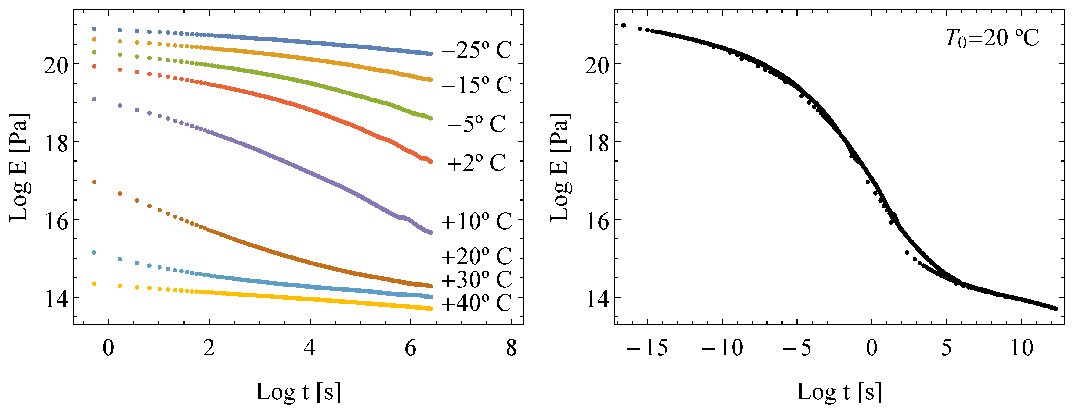
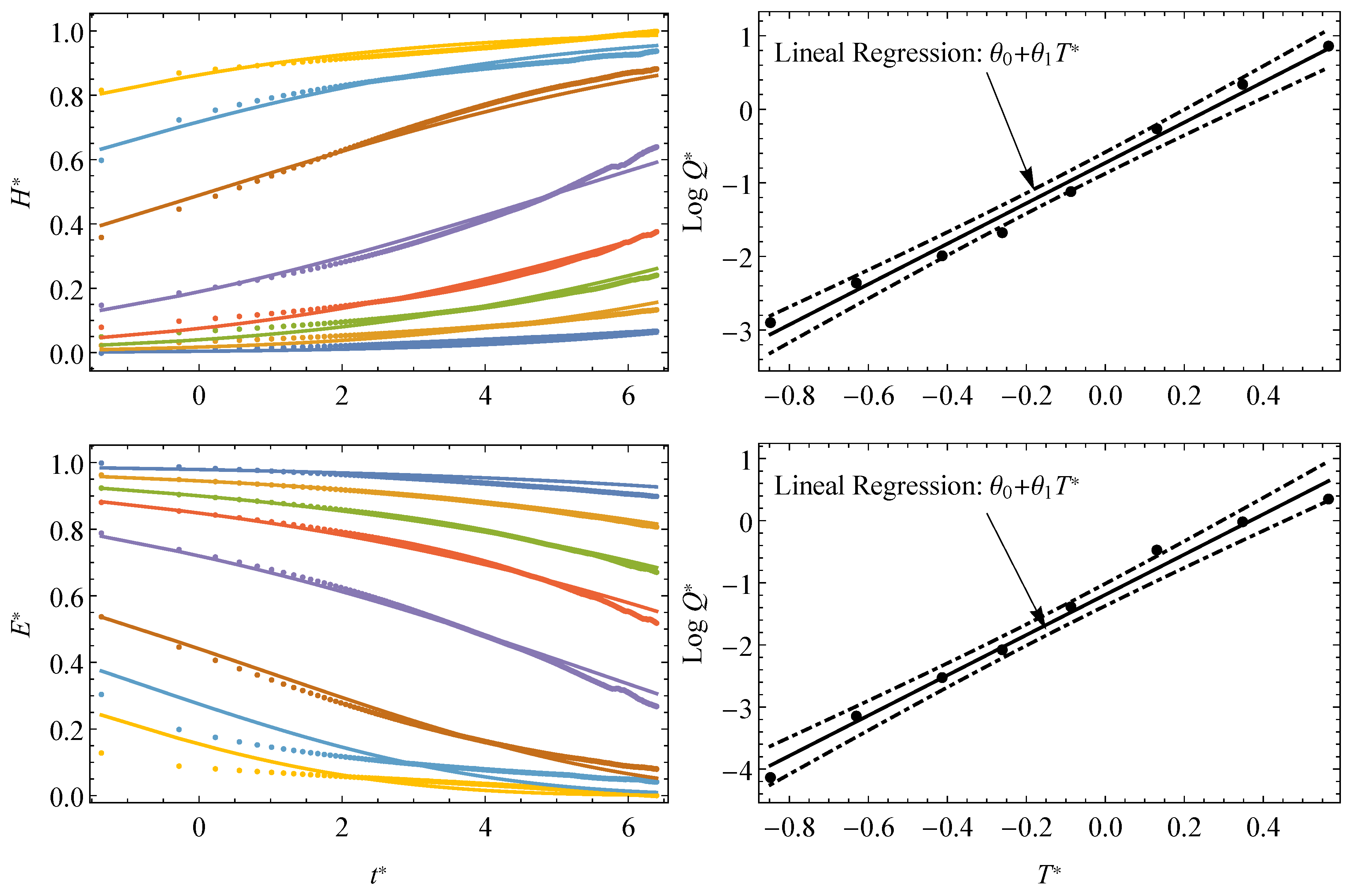
4.2. Short-Term Relaxation Curves Estimation
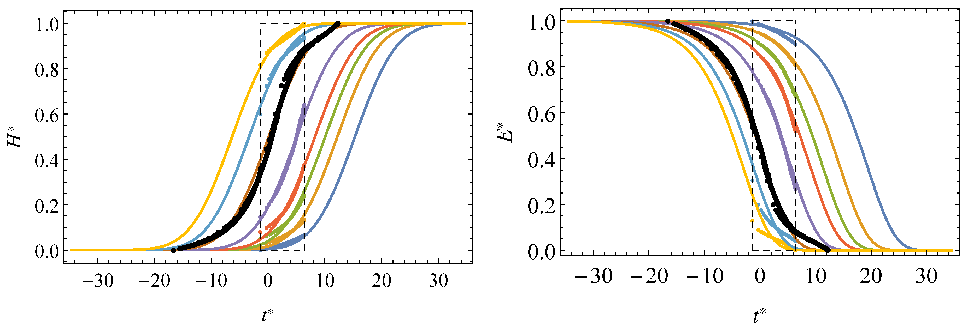
4.3. Master Curves Prediction
5. Discussion
- (a)
- Dimensional consistency. A robust scientific basis is considered for building TTS models according to good practice in what concerns the dimensional analysis of the involved variables for viscoelastic characterization. As a consequence, the proposed TTS model and their parameters are insensitive to the system of units selected for the fundamental physical magnitudes.
- (b)
- Analytical definition of field. From a practical viewpoint, the analytical definition of the viscoelastic modulus, , as a cdf, represents the most important contribution of the proposed approach allowing the field to be fully defined by fitting the experimental short-term relaxation curves over the whole range of time (i.e., as master curves) and temperatures.
- (c)
- Statistical approach of viscoelastic modulus. The proposed approach contributes to broadening the theoretical framework in which the TTS principle and their models are developed and applied. As a matter of fact, a physical and phenomenological conceptualization of the relaxation phenomenon as statistical cdfs is now available. The already acquired mathematical knowledge about statistical cdfs favors further development of advanced methods for modeling and designing components with viscoelastic behavior.
- (d)
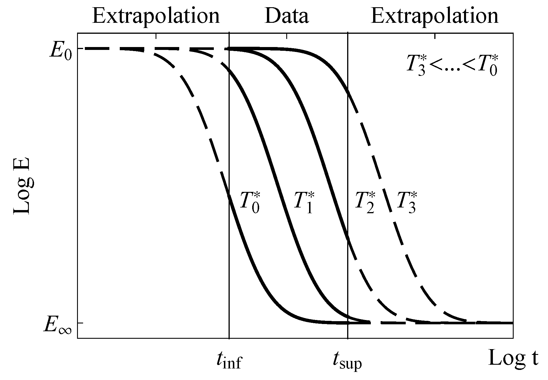
- Independence of the reference temperature. Due to the analytical definition of the field over the whole range of time, the parametric family of master curves are obtained independently of the reference temperature for the first derived of them, satisfying which may be conveniently called a certain uniqueness condition.
- (e)
- Analytical definition of the Q shift factor. Classical TTS models are based on discretional assumptions, which allow analytical definitions of the shift factor, Q, to be derived, such as the linearity of free-volume concept in the theoretical development of the WLF model. In the new model proposed, the shift factor is derived analytically, free of gratuitous assumptions, based on the theory of the functional equations once the TTS model is defined.
- (f)
- Simultaneous definition of the master curves and short-term curves. The proposed model allows the master curves to be derived directly from the fitting of the experimental short-term relaxation tests, which avoids the hand-made pre-fittings required in the application of current TTS models. Likewise, master curves at different temperatures can be predicted based on the analytical definition of the shift factor, in order to satisfy the uniqueness condition.
- (g)
- Full applicability of the proposed models over all the range of temperatures. The applicability of the displacement factor in current models is limited as the required combination of two models for the definition of this factor depending of the range of temperatures analyzed. On the contrary, the proposed model is applicable over the whole range of temperatures, avoiding different definitions of Q for each viscoelastic characterization.
- (h)
- Non-overlapping constraint. The current methodologies require a certain overlapping of the short-time relaxation curves, which must be at least one decade, known as the “rule of thumb” in literature. In turn, the proposed methodology does not require the overlapping among these short-time curves which is an important advantage.
- (i)
- The proposed approach proves to be valid over the whole possible range of temperatures, a question of practical interest, unsatisfactorily accomplished by commonly used TTS methods, such as the Williams–Landel–Ferry model.
6. Conclusions
- −
- A previous dimensional analysis of the variables involved in relaxation viscoelastic phenomena provides a robust basis for building TTS models that satisfy the necessary dimensional consistency.
- −
- The proposed methodology allows the analytical expression of the relaxation viscoelastic modulus, , from short to long-term time periods to be derived for any temperature while avoiding the typical hand-made pre-fittings observed by current practical methods.
- −
- Based on a statistical similitude in the evolution of the viscoelastic phenomenon, two suitable models, namely based on the normal and the Gumbel cumulative distribution functions (with possible extension to the bi-parametric Weibull) are proposed, as possible candidates for representing the relaxation function, . In this way the field is analytically defined whereas the temperature effect is found to act as a change in the scale parameter of those distributions.
- −
- The use of the normal model is justified from strain considerations and consequent application of the statistical limit central theorem while the Gumbel model is particularly recommended when maximal or minimal values of the relaxation modulus of the material are determined, as for instance, when design is concerned with short or large loading times. In such cases, asymptotic fitting of the extreme values of the relaxation function based on a Gumbel function provides more reliable parameter estimation.
- −
- Master curves for any temperature other than those used in the test are easily obtained from the analytical definition of the shift factors. In this way, short- and long-term prediction of the relaxation modulus is feasible, irrespective of the temperature history the component is subject to. The functional expression of the latter is derived from functional equations theory without any arbitrary assumption.
Author Contributions
Funding
Conflicts of Interest
Abbreviations
| Relaxation modulus as a function of time and temperature | |
| Normalized relaxation modulus as a function of normalized time and temperature | |
| Initial or elastic relaxation modulus | |
| Initial or elastic relaxation modulus | |
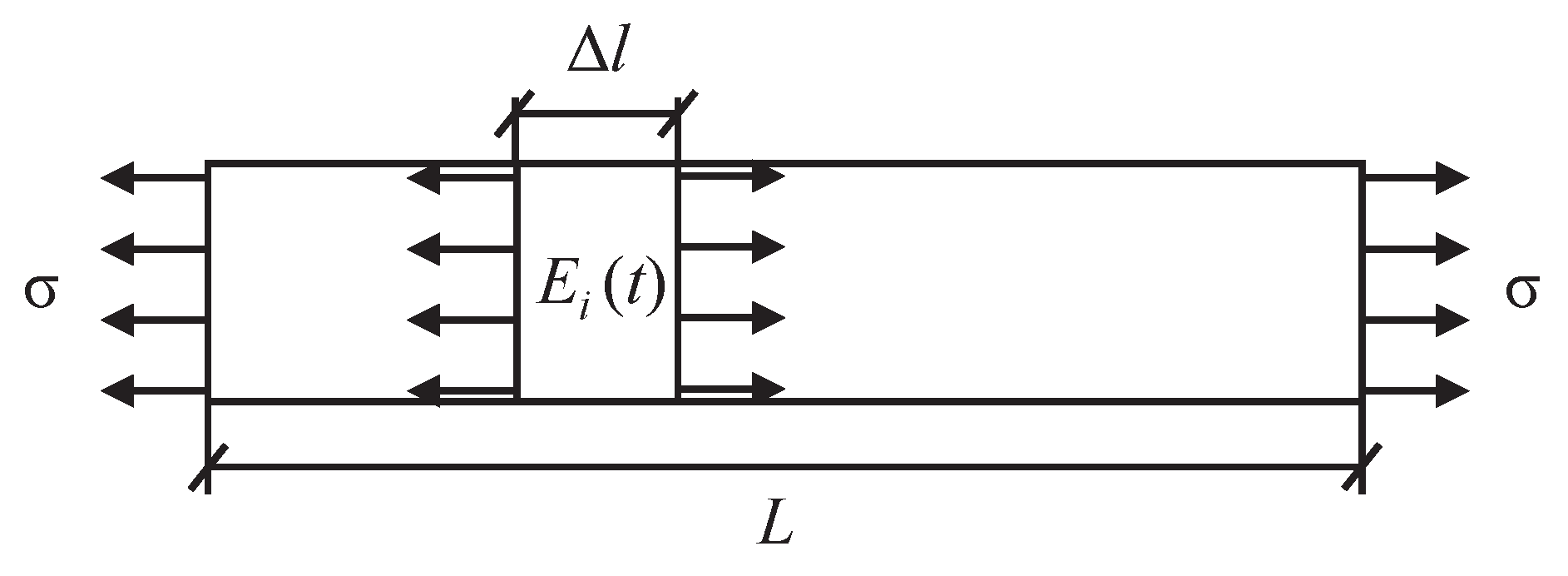
| L | Total specimen length |
| t | Time |
| T | Temperature |
| Transition temperature | |
| Rubbery temperature | |
| Reference temperature | |
| GEV | Generalized extreme value |
| TTS | Time–Temperature Superposition |
| WLF | Williams–Landel–Ferry |
| TTS | Time–Temperature Superposition |
| Displacement as a function of time | |
| Length of each of the n subelements in which the specimen of length L is virtually subdivided |
References
- Findley, W.N.; Lai, J.S.; Onaran, K. Creep and Relaxation of Nonlinear Viscoelastic Materials. With and Introduction to Linear Viscoelasticity; Dover Publications: New York, NY, USA, 1976. [Google Scholar]
- Ferry, J.D. Viscoelastic Properties of Polymers, 3rd ed.; John Wiley and Sons: Hoboken, NJ, USA, 1980. [Google Scholar]
- Tschoegl, N. The Phenomenological Theory of Linear Viscoelastic Behavior. An Introduction, 1st ed.; Springer: Berlin/Heidelberg, Germany, 1989. [Google Scholar]
- Lakes, R. Viscoelastic Materials, 1st ed.; Cambridge University Press: Cambridge, UK, 2009. [Google Scholar]
- Williams, M.; Landel, R.; Ferry, J. The temperature dependence of relaxation mechanisms in amorphous polymers and other glass-forming liquids. J. Am. Chem. Soc. 1955, 77, 3701–3707. [Google Scholar] [CrossRef]
- Knauss, W.G. The sensitivity of the time-temperature shift process to thermal variations—A note. Mech. Time Depend. Mater. 2008, 12, 179–188. [Google Scholar] [CrossRef]
- Gergesova, M.; Zupančič, B.; Saprunov, I.; Emri, I. The closed form t-T-P shifting (CFS) algorithm. J. Rheol. 2011, 55, 1–16. [Google Scholar] [CrossRef]
- Tanaka, T. Experimental Methods in Polymer Science. Modern Methods in Polymer Research and Technology, 1st ed.; Polymers, Interfaces and Biomaterials; Academic Press: New York, NY, USA, 2012. [Google Scholar]
- Pelayo, F.; Lamela-Rey, M.; Muniz-Calvente, M.; López-Aenlle, M.; Álvarez Vázquez, A.; Fernández-Canteli, A. Study of the time-temperature-dependent behaviour of PVB: Application to laminated glass elements. Thin-Walled Struct. 2017, 119, 324–331. [Google Scholar] [CrossRef]
- Buckingham, E. The principle of similitude. Nature 1915, 96, 396–397. [Google Scholar] [CrossRef]
- Aczél, J. On scientific laws without dimensional constants. J. Math. Anal. Appl. 1986, 119, 389–416. [Google Scholar] [CrossRef]
- Castillo, E.; Ruiz-Cobo, M.R. Monographs and Tetxtbooks in Pure and Applied Mathematics. In Functional Equations and Modelling in Science and Engineering; Marcel Dekker Inc.: New York, NY, USA, 1992; Volume 161. [Google Scholar]
- Castillo, E.; Iglesias, A.; Ruiz-Cobo, R. Functional Equations in Applied Sciences, 1st ed.; Elsevier Science: Amsterdam, The Netherlands, 2004. [Google Scholar]
- McCrum, N.G.; Morris, E.L. On the measurement of the activation energies for creep and stress relaxation. Proc. R. Soc. A 1964, 281, 258–273. [Google Scholar]
- Stouffer, D.C.; Wineman, A.S. Linear viscoelastic materials with environmental dependent properties. Int. J. Eng. Sci. 1971, 9, 193–212. [Google Scholar] [CrossRef][Green Version]
- Gross, B. Time-temperature superposition principle in relaxation theory. J. Appl. Phys. 1969, 40, 3397. [Google Scholar] [CrossRef]
- Bogdanoff, J.L.; Kozin, F. Effect of length on fatigue life of cables. J. Eng. Mech. 1987, 113, 925–940. [Google Scholar] [CrossRef]
- Castillo, E.; Fernández-Canteli, A.; Ruiz-Tolosa, J.R.; Sarabia, J.M. Statistical models for analysis of fatigue life of long elements. J. Eng. Mech. 1988, 116, 1036–1049. [Google Scholar] [CrossRef]
- Castillo, E.; Fernández-Canteli, A. A Unified Statistical Methodology for Modeling Fatigue Damage, 1st ed.; Springer Netherlands: Dordrecht, The Netherlands, 2009. [Google Scholar]
- Castori, G.; Speranzini, E. Fracture strength prediction of float glass: The coaxial double ring test method. Constr. Build. Mater. 2019, 225, 1064–1076. [Google Scholar] [CrossRef]
- Muñiz-Calvente, M.; Ramos, A.; Pelayo, F.; Lamela, M.J.; Álvarez-Vázquez, A.; Fernández-Canteli, A. Probabilistic failure analysis for real glass components under general loading conditions. Fatigue Fract. Eng. Mater. Struct. 2019, 46, 1283–1291. [Google Scholar] [CrossRef]
- Galambos, J. The Asymptotic Theory of Extreme Order Statistics; John Wiley & Sons: Hoboken, NJ, USA, 1978. [Google Scholar]
- Castillo, E. Extreme Value Theory in Engineering, 1st ed.; Academic Press: New York, NY, USA, 1988. [Google Scholar]
- Castillo, E.; Hadi, A.S.; Balakrishnan, N.; Sarabia, J.M. Extreme Value and Related Models with Applications in Engineering and Science, 1st ed.; Series in Probability and Statistics; Wiley: Hoboken, NJ, USA, 2004. [Google Scholar]
- Hadi, A.S.; Chatterjee, S. Regression Analysis by Example, 5th ed.; Wiley Series in Probability and Statistics; John Wiley & Sons: Hoboken, NJ, USA, 2012. [Google Scholar]


| Model | Error | |||||||
|---|---|---|---|---|---|---|---|---|
| Normal | 20.99 | 13.69 | −1.37 | 10.54 | 11.54 | −1.86 | 1.52 | 104.08 |
| Gumbel | 21.44 | 13.69 | −1.37 | 6.97 | — | −0.77 | 2.59 | 159.95 |
© 2020 by the authors. Licensee MDPI, Basel, Switzerland. This article is an open access article distributed under the terms and conditions of the Creative Commons Attribution (CC BY) license (http://creativecommons.org/licenses/by/4.0/).
Share and Cite
Álvarez-Vázquez, A.; Fernández-Canteli, A.; Castillo Ron, E.; Fernández Fernández, P.; Muñiz-Calvente, M.; Lamela Rey, M.J. A Novel Approach to Describe the Time–Temperature Conversion among Relaxation Curves of Viscoelastic Materials. Materials 2020, 13, 1809. https://doi.org/10.3390/ma13081809
Álvarez-Vázquez A, Fernández-Canteli A, Castillo Ron E, Fernández Fernández P, Muñiz-Calvente M, Lamela Rey MJ. A Novel Approach to Describe the Time–Temperature Conversion among Relaxation Curves of Viscoelastic Materials. Materials. 2020; 13(8):1809. https://doi.org/10.3390/ma13081809
Chicago/Turabian StyleÁlvarez-Vázquez, Adrián, Alfonso Fernández-Canteli, Enrique Castillo Ron, Pelayo Fernández Fernández, Miguel Muñiz-Calvente, and María Jesús Lamela Rey. 2020. "A Novel Approach to Describe the Time–Temperature Conversion among Relaxation Curves of Viscoelastic Materials" Materials 13, no. 8: 1809. https://doi.org/10.3390/ma13081809
APA StyleÁlvarez-Vázquez, A., Fernández-Canteli, A., Castillo Ron, E., Fernández Fernández, P., Muñiz-Calvente, M., & Lamela Rey, M. J. (2020). A Novel Approach to Describe the Time–Temperature Conversion among Relaxation Curves of Viscoelastic Materials. Materials, 13(8), 1809. https://doi.org/10.3390/ma13081809