Electricity Self-Sufficient Community Clustering for Energy Resilience

Abstract

Local electricity generation and sharing has been given considerable attention recently for its disaster resilience and other reasons. However, the process of designing local sharing communities (or local grids) is still unclear. Thus, this study empirically compares algorithms for electricity sharing community clustering in terms of self-sufficiency, sharing cost, and stability. The comparison is performed for all 12 months of a typical year in Yokohama, Japan. The analysis results indicate that, while each individual algorithm has some advantages, an exhaustive algorithm provides clusters that are highly self-sufficient. The exhaustive algorithm further demonstrates that a clustering result optimized for one month is available across many months without losing self-sufficiency. In fact, the clusters achieve complete self-sufficiency for five months in spring and autumn, when electricity demands are lower.

1. Introduction

While electricity is a fundamental requirement for sustainable urban development, electricity supply can be interrupted by natural or man-made disasters, including earthquakes and cyber-attacks. In Japan, the nuclear power plants in Fukushima were seriously damaged by the 2011 Great East Japan Earthquake, and a massive blackout occurred in the Tokyo Metropolitan area.

Distributed (or decentralized) generation systems [1] are a useful alternative to centralized generation systems. A distributed system generates electricity locally using renewables, and distributes the electricity to a local grid. Decentralized generation systems, which increase energy resilience and decrease carbon emission, have been given considerable attention in recent years (see, [2]). Implementation of decentralized systems would be particularly important in Asian countries, where populations are increasing rapidly, while natural disasters are simultaneously increasing in frequency and intensity owing to climate change (see, e.g., [3]).

A distributed electricity generation system consists of the following elements: (i) electricity generators; (ii) electricity storage; and (iii) a local grid. Electricity can be generated by use of wind generators, photovoltaic (PV) panels, fuel cell generators, and so on. These options are desirable because of their stability and low emissions [4], and although they are somewhat costly [5], the costs have been declining. For instance, the cost of PV electricity generation is now competitive with conventional, centralized electricity generation [6]. On the other hand, regarding electricity storage, use of electric vehicle (EV) batteries has extensively been discussed (e.g., [7,8,9]) and reviewed by [10].

A decentralized electricity production system that integrates PV for generation and EVs for storage is a promising option. In the vehicle-to-community (V2C) system [11,12,13], electricity generated by mass-adopted PVs is stored in EV batteries, and then shared within the local community.

The potential for using EV batteries as electricity storage devices has been extensively discussed in recent years (e.g., [14,15]). The battery capacity of the Leaf, a popular EV produced by Nissan Motor Co., Ltd. [16], is 30 kWh, whereas the daily household electricity consumption in Japan was 14.5 kWh in 2014 (source: [17]). Thus, one battery could support typical household consumption for two days. Sharing electricity in EV batteries through the V2C system is especially helpful in an emergency or during the daily peak demand.

Yamagata and Seya [12] demonstrated that a V2C system provides sufficient electricity for households in many of the local communities in Yokohama, Japan. However, they also showed a significant regional imbalance, with the storage capacity (i.e., the number of EVs) being insufficient in some regions and excessive in others. Their study highlights the importance of designing a local grid that balances the local storage capacity with the local PV generation ability. Unfortunately, how to design such local communities is largely unexplored.

As a first step towards energy self-sufficiency, this study compares community clustering algorithms, and discusses how to design electricity self-sufficient local communities for the V2C system. The paper is organized as follows: Section 2 describes situations relating to EV and PV in Japan; Section 3 explains the clustering algorithms used; Section 4 empirically compares these algorithms, and clarifies advantages and disadvantages of each algorithm in terms of the sharing community clustering; and, finally, Section 5 contains discussions on the analysis results, and our conclusions.

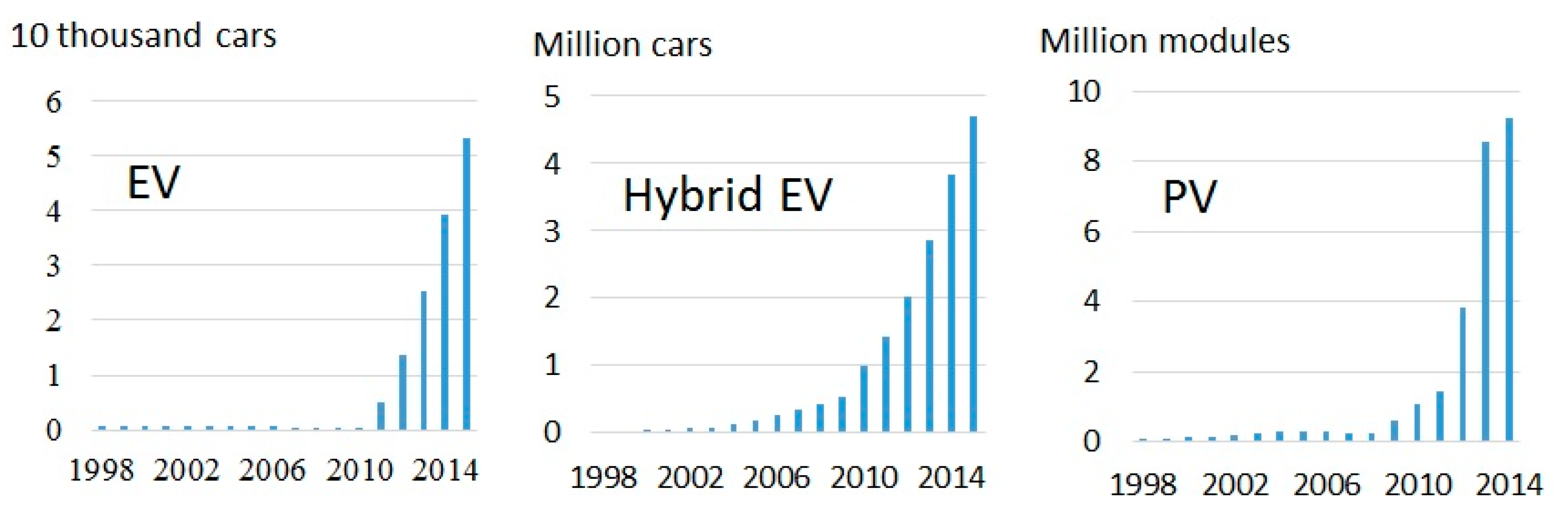
2. EV and PV in Japan

Figure 1 plots the numbers of EVs, hybrid EVs (HEV, vehicles that use both EV and a combustion engine, switching based on driving conditions), and PVs in Japan. As can be seen, EV use increased rapidly after the Automotive Industry Strategy was launched in 2010, encouraging EV production and promotion. PV use increased rapidly beginning around 2009, when a surplus PV electricity-purchasing scheme began. The increase accelerates again around 2012, when the purchasing scheme changed to the feed-in-tariff (FiT), which purchases all PV electricity. Although the market penetration percentages of EV and HEV are still only 0.19% and 7.76%, respectively, in 2015 [18], rapidly-increasing use of EV, HEV, and PV indicates good potential for the V2C system in Japan.

A number of cities have been selected as test sites for local grids using EV and PV [19]. Viability of widespread V2C systems depends on continued economic and technological progress for EV and PV. For instance, a recent rapid reduction in solar panel prices (see, [19]) significantly increases the viability from an economic perspective.

This study assumes a best-case scenario where all cars are replaced with EVs, and PVs are installed on the rooftops of all detached houses (i.e., each house operates as an EV charging station, and electricity is transmitted to a local grid by connecting the EV battery to the grid). Although this scenario is difficult to achieve, it should help clarify to what extent a V2C system is capable of contributing to energy resilience. By focusing on the maximum potential of V2C systems, future spread of EV and PV can be directed to provide the maximum benefit.

3. Community Clustering for the V2C System

3.1. Problem Setting

We represent the electrical grid in a study area (in our case, it is Yokohama, Japan; see Section 4) as a graph G = (V, E), where the nodes, V, represent the 250-m grids in the target area and the edges, E, represent their neighboring relations. Our objective is to partition the graph G into self-sufficient sub-graphs or local communities, {G₁ = (V₁, E₁), G₂ = (V₂, E₂), G_n = (V_n, E_n)}.

The i-th local community, G_i, is electrically self-sufficient if the storage capacity C(G_i) and the PV electricity supply are well balanced. We assume that only surplus electricity, S(G_i) − D(G_i), is stored, where S(G_i) is the PV electricity supply, and D(G_i) is the household electricity demand. The balance can be quantified by the difference between the capacity and the surplus electricity, |w(G_i)|, where w(G_i) is formulated as follows:

$$w(G_i)=C(G_i)-[S(G_i)-D(G_i)]$$

(1)

where w(G_i) measures the storage availability |w(G_i)| is small if the storage capacity matches the surplus electricity well in each community. In other words, communities minimizing |w(G_i)| are self-sufficient in terms of storage efficiency.

In addition to the storage efficiency, the electricity transmission cost must also be minimized for efficient electricity sharing. Thus, the following sub-sections introduce algorithms that identify local communities considering both the storage efficiency and the sharing cost.

Two approaches are possible to solve this clustering problem: (i) maximizing the storage efficiency while constraining the transmission cost; and (ii) minimizing the transmission cost while constraining the storage efficiency.

There are two representative approaches to solve clustering problems: the graph partitioning and meta-heuristic approaches. The former optimizes positions of partitions in a graph determining the transmission cost, whereas the latter can maximize the storage efficiency directly, which is our principal interest. This difference leads to different objective functions, as explained later. The remainder of this section formulates graph partitioning and meta-heuristic approaches for clustering communities with self-sufficient electricity production.

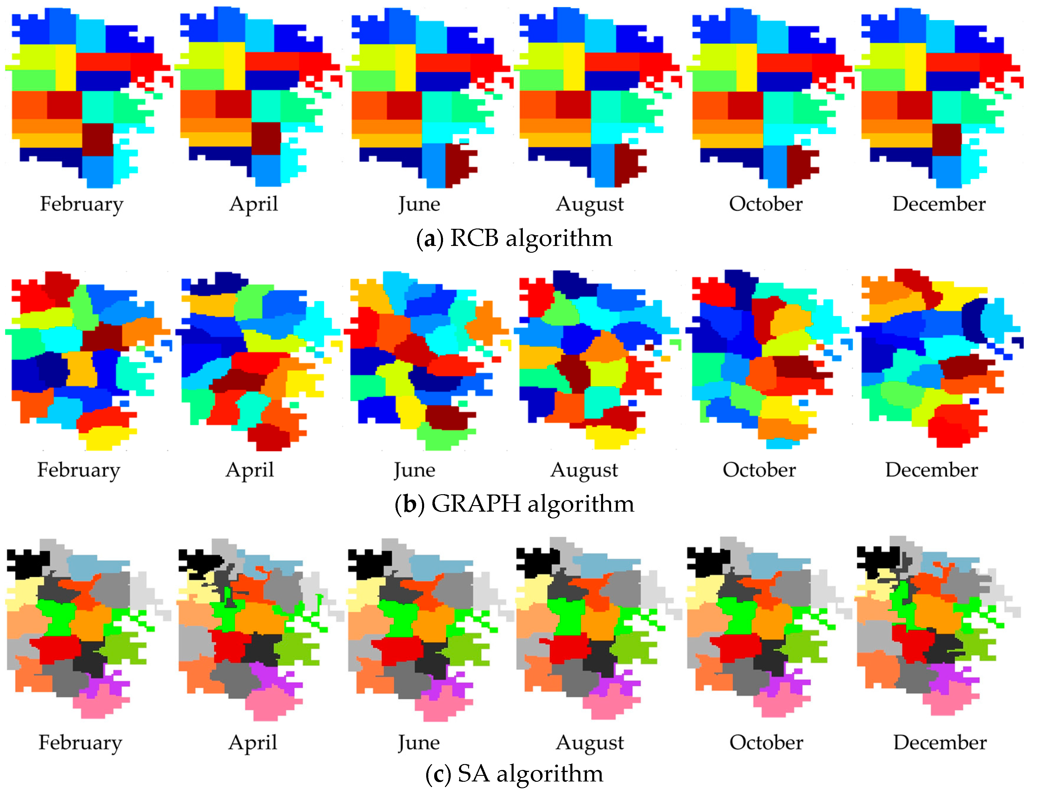
3.2. Graph Partitioning Algorithms

We first write the electricity transmission cost in G as follows:

$$O_g=\mathsf{\alpha }{\displaystyle \sum _{i=1}^n|V_i{|}^2+\mathsf{\beta }\left|E\underset{i=1}{\stackrel{n}{\cup }}{E}_i\right|}$$

(2)

where α and β are coefficients such that α + β = 1. |Vi|² counts the number of node pairs within each local community (sub-graph), which we use as a proxy of the transmission cost within G_i. |Vi|² grows rapidly as the size of G_i increases. In other words, the first term, describing the internal transmission cost, is small when all of the clusters are reasonably small. The second term counts the number of edges across communities (sub-graphs), which is small if the clusters are circular-shaped. The transmission cost, Equation (2), is small if clusters are small and circular-shaped.

We attempt to minimize Equation (2) with a self-sufficiency constraint: |w(G_i)| < k, where k is a given threshold. The minimization identifies local clusters with low sharing costs and high self-sufficiency. The problem is formulated as follows:

Definition 1. 

(Graph clustering problem): Given graph G = (V, E), where each node n_i is labeled with weight w(n_i) and threshold k, the graph clustering problem finds a set of sub-graphs {G₁ = (V₁, E₁), G₂ = (V₂, E₂), …, G_n = (V_n, E_n)} such that

• V = ${\cap }_i{V}_i$ where V_i $\cap$ V_j = ø if i $\ne$ j,
• For every graph partition {G′₁, G′₂, …, G′_n}, O_g(G₁, G₂, …, G_n) ≤ O_g(G′₁, G′₂, …, G′_n),
• For every subgraph G_i, |w(G_i)| < k.

Among the several algorithms available to solve this problem, we apply the following standard ones: the recursive coordinate geometric bisection (RCB) algorithm ([22]), which allows vertical and horizontal partitioning only, and the multi-level graph (GRAPH) algorithm ([23,24,25]), which is a more general partitioning algorithm.

The clustering procedure of the RCB algorithm is summarized as follows:

• The graph is split vertically or horizontally into two sub-graphs of nearly equal sizes.
• Step 1 is iterated for each sub-graph.

Although this is a simple approximation, the RCB algorithm is preferable for clusters that satisfy the self-sufficiency constraint.

Next, we describe a general graph partition algorithm that supports irregular partitions of the graph while explicitly controlling the edge connectivity. It can partition graphs into subgraphs that maintain the balance of the sum of the weights (Equation (3)):

$$w(G_i)\le (1+\mathsf{\epsilon }){\displaystyle \sum _i\frac{w(G_i)}{n}}\times \forall i$$

(3)

where n is the number of subgraphs. Minimizing edge connections between subgraphs is accomplished by:

$$\left|E(G){\displaystyle \underset{i=1}{\overset{n}{\cup }}E(G_i)}\right|$$

(4)

We assumed ε = 0.35 based on some preliminary analyses. The clustering procedure using the GRAPH algorithm is summarized as follows:

• Construct a smaller summarization of a graph by aggregating nodes and edges in the graph.
• Perform a graph partitioning procedure on the summarized graph.
• Propagate the computed partition back to the original graph.
• Repeat this process on the resulting partitions as needed.

While the GRAPH algorithm, which allows general-shaped clusters, may be more preferable in terms of flexibility, it can be slow relative to the RCB algorithm.

3.3. Meta-Heuristic Optimization

While the RCB and the GRAPH algorithms do not perform exhaustive optimizations, but rather fast approximations, it is unclear to what extent exhaustiveness is important for efficient detection of self-sufficient clusters. Hence, a simulated annealing-based (SA; [26]) exhaustive optimization was also used.

SA is a probabilistic meta-heuristic algorithm. It searches the global optimum by gradually reducing the cooling parameter: if the parameter is large, large jumps in the search space are allowed for each iteration, but as the parameter becomes smaller, the jumps are restricted to be smaller and smaller. This optimization scheme effectively avoids converging to a local optimum. In particular, the probability of converging to the global optimum approaches 1 as the decay speed of the cooling parameter slows. The SA algorithm is more flexible than the RCB and the GRAPH algorithms. In addition, the assumption of a gridded neighborhood structure, which can make an algorithm less flexible, is not needed for this algorithm, and nodes (V) and edges (E) do not appear in the subsequent equations. Since it is so flexible and thorough, the SA algorithm can be exceedingly slow.

While the graph partitioning algorithms evaluate electricity-sharing cost in each graph, the SA algorithm evaluates the sharing cost using the circularity (Equation (5)):

$$\mathit{Circle}={\displaystyle \sum _i\left(1-\sqrt{4\pi \frac{|a(G_i)|}{p{(G_i)}^2}}\right)}$$

(5)

where a(G_i) and p(G_i) are geographical measurements, the former being the area of the cluster G_i, which consists of 250-m grids, and the latter being the perimeter. Circle approaches zero if clusters are circular-shaped, and 1 if they are non-circular-shaped. Since the inter-point distance between arbitrary points in a circle region is smaller than those in any other shaped regions, Circle can be used as a measure of the electricity-sharing cost.

We minimize the following cost function in the SA algorithm:

$$O_s={\displaystyle \sum _i|w(G_i)|}+\mathsf{\lambda }Circle$$

(6)

where λ is a given parameter, and the first and second terms quantify the storage sufficiency (or self-sufficiency) and the electricity sharing cost, respectively.

The problem to be solved by the SA algorithm is formulated as follows:

Definition 2. 

Meta-heuristic graph clustering problem: Given graph G = (V, E), where each node n_i is labeled with weight w(n_i), the meta-heuristic clustering problem finds a set of sub-graphs {G₁ = (V₁, E₁), G₂ = (V₂, E₂), …, G_n = (V_n, E_n)} such that:

• V = ${\cap }_i{V}_i$ where V_i $\cap$ V_j = ø if i $\ne$j,
• For every graph partition {G′₁, G′₂, …, G′_n}, O_s(G₁, G₂, ..., G_n) $\le$ O_s(G′₁, G′₂, ..., G′_n).

w(G_i) does not appear in Definition 2 because it is embedded in O_s. SA solves this cluster optimization problem as follows (see, [27,28]):

• Set initial M sub-graphs (local communities), and calculate the cost O_s = O_s(G₁, G₂, ..., G_m).
• Detach a node n_i from the corresponding subgraph G_i, and merge it into another subgraph G′_i, then, calculate the cost O′_s = O_s(G′₁, G′₂, ..., G′_m).
• If O_s $\ge$ O′_s, the change is accepted. Otherwise, the change is accepted with a probability, which is evaluated by exp{−(O′_s − O _s)/T}, where T is the cooling parameter that controls the acceptance probability.
• Iterate steps 2 and 3 alternately until O′_s converges.

To find the global optimum, the cooling parameter T needs be reduced gradually across iterations. We define it by T = γ^k × T₀, where T₀ = 10⁵. The probability that an SA algorithm converges to the global optimum approaches 1.0 as γ approaches 1.0 [26]. Thus, γ is set at 0.9999.

In summary, the RCB algorithm is the fastest, but least flexible, the SA algorithm is the slowest, but most flexible, and the GRAPH algorithm falls between the other two in terms of both computational time and flexibility. The next section applies the three algorithms to clustering of communities with self-sufficient electricity production in Yokohama, Japan.

4. Energy Self-Sufficient Community Clustering in Yokohama, Japan

The RCB, GRAPH, and SA algorithms are applied to detect self-sufficient clusters in Yokohama, Japan. Yokohama is located about 30 min south of the center of Tokyo. The population was about 3.7 million in 2015, the second largest municipality in Japan. Here, as a way to consider seasonal differences, clustering was performed for every month.

To perform the clustering, we first need to evaluate C(G_i), S(G_i), and D(G_i), which determine w(G_i). Section 4.1 explains how to calculate these three values in 250-m grids for each month, and Section 4.2 explains the implementation of the clustering algorithms.

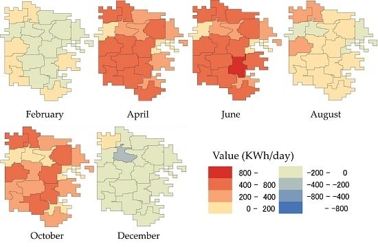
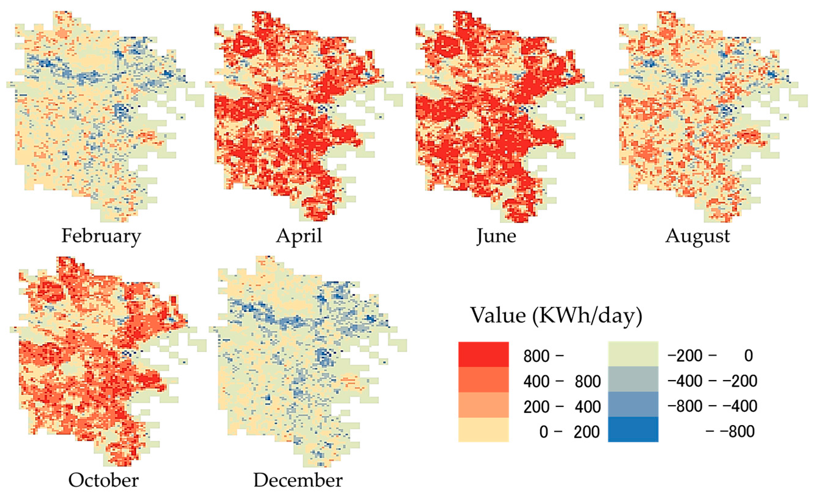
4.1. Estimation of Storage Sufficiency in Month m: w_m(G_i)

4.1.1. Calculation of the Storage Capacity: C(G_i)

We use cars for electricity storage in our V2C analysis. The number of cars not in use in each 250-m grid was estimated by a simulation using MATsim, which is an open source agent-based transport simulator developed by researchers in ETH Zurich (Eidgenössische Technische Hochschule Zürich), Switzerland, and TU Berlin (Technische Universität Berlin), Germany. For more details about MATsim, see [29]. In this simulation, daily movement of people in Yokohama were simulated using MATsim with inputs of road network data (source: National Digital Road Map Database), data recording 722,000 people’s actual travel behaviors during a given few days from October to December (source: Person Trip Survey in 2008), and the number of registered cars in Yokohama. The number of cars not in use was estimated based on the trip duration and arrival time of each agent during the simulation. Multiplying this number by the battery storage capacity produced the total electricity storage capacity for a given grid. For the storage capacity, we assumed 30 kWh that is the capacity of Nissan Leaf, which is a representative EV.

4.1.2. Calculation of the Potential PV Electricity Supply in Month m: S_m(G_i)

Following [30], the electricity PV supply in m-th month in i-th cluster, PV_m(G_i), is estimated by Equation (7):

$$P{V}_m(G_i)=I\times \mathsf{\tau }\times {roof}^{PV}(G_i)\times {\mathsf{\eta }}_{pc}\times K_{m,pt}\times T$$

(7)

where I is the total solar irradiance (kWh/m²/h) as calculated by the METPV-2 database [30], τ is the array conversion efficiency (=0.1), roof^PV(G_i) is the installation area in i-th cluster (m²), η_pc is the efficiency of the power conditioner (=0.95), K_m,pt is the temperature correction coefficient set for each month m (e.g., May: 0.92; August: 1.00), and T is the performance ratio (=0.89).

4.1.3. Calculation of the Electricity Demand in Month m: D_m(G_i)

The monthly household electricity demand in the i-th cluster, D_m(G_i), is estimated by F(G_i) × b_m, where F(G_i) is the total floor area in the i-th grid (source: Zenrin Z-map TOWN II), and b_m is the unit electricity demand in each month, which was published by the Japan Institute of Energy in 2008.

4.1.4. Storage Availability in Month m: w_m(G_i)

Figure 2 plots the estimated storage availability in the six months. This figure suggests that the availability decreases in summer and winter, when electricity demands for cooling or heating are large. In each month, storage availability is imbalanced spatially, so some areas have excess storage, while others have insufficient storage. Community clustering would be helpful to moderate the imbalance and increase self-sufficiency.

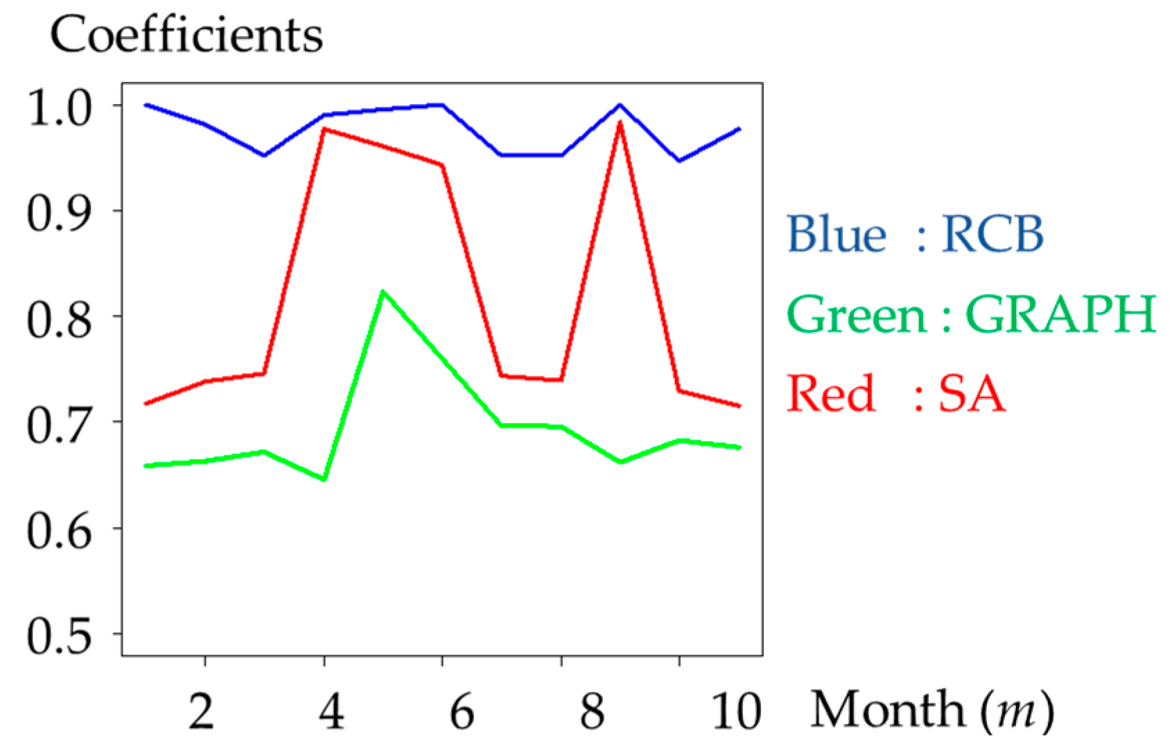
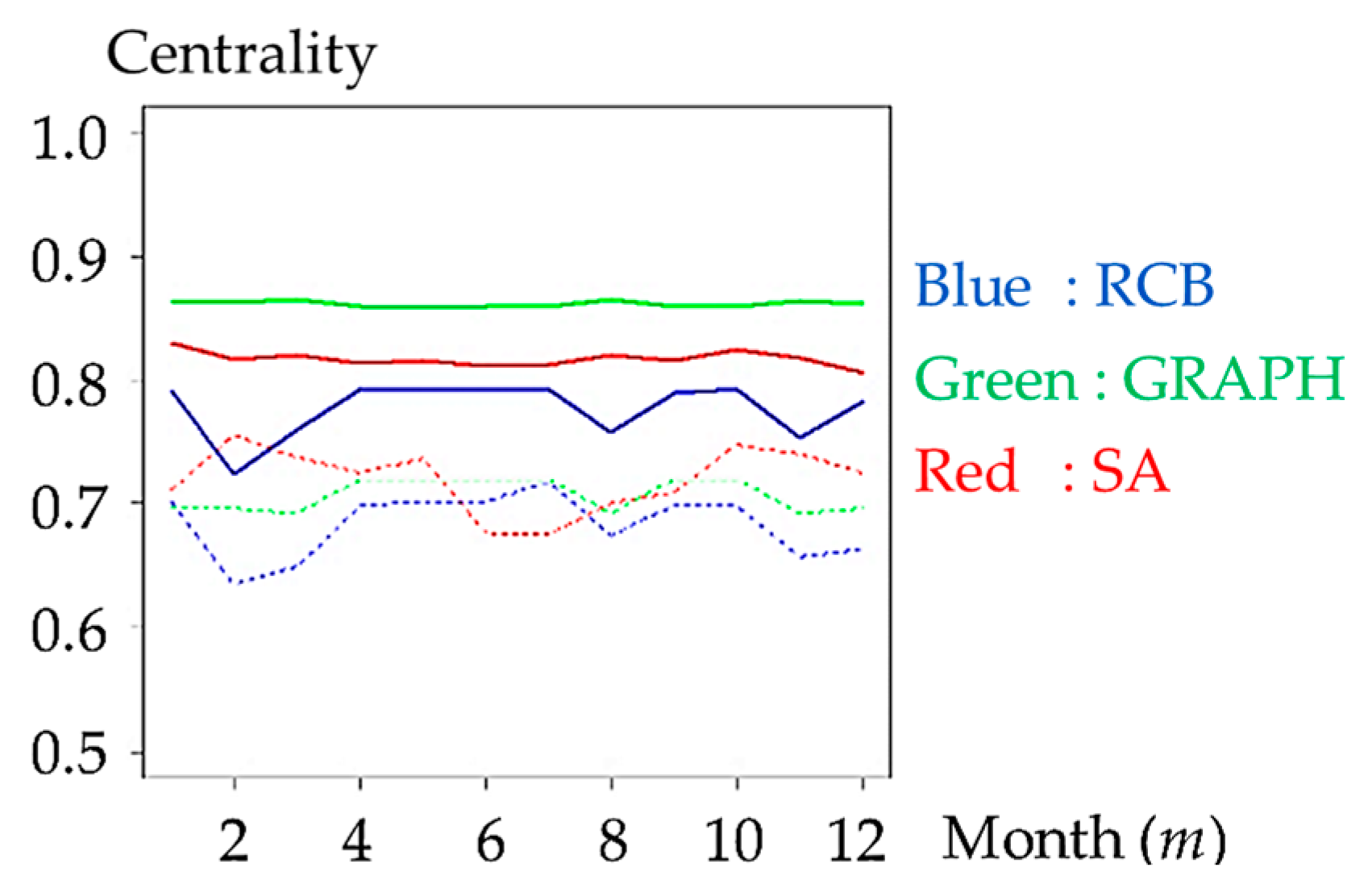
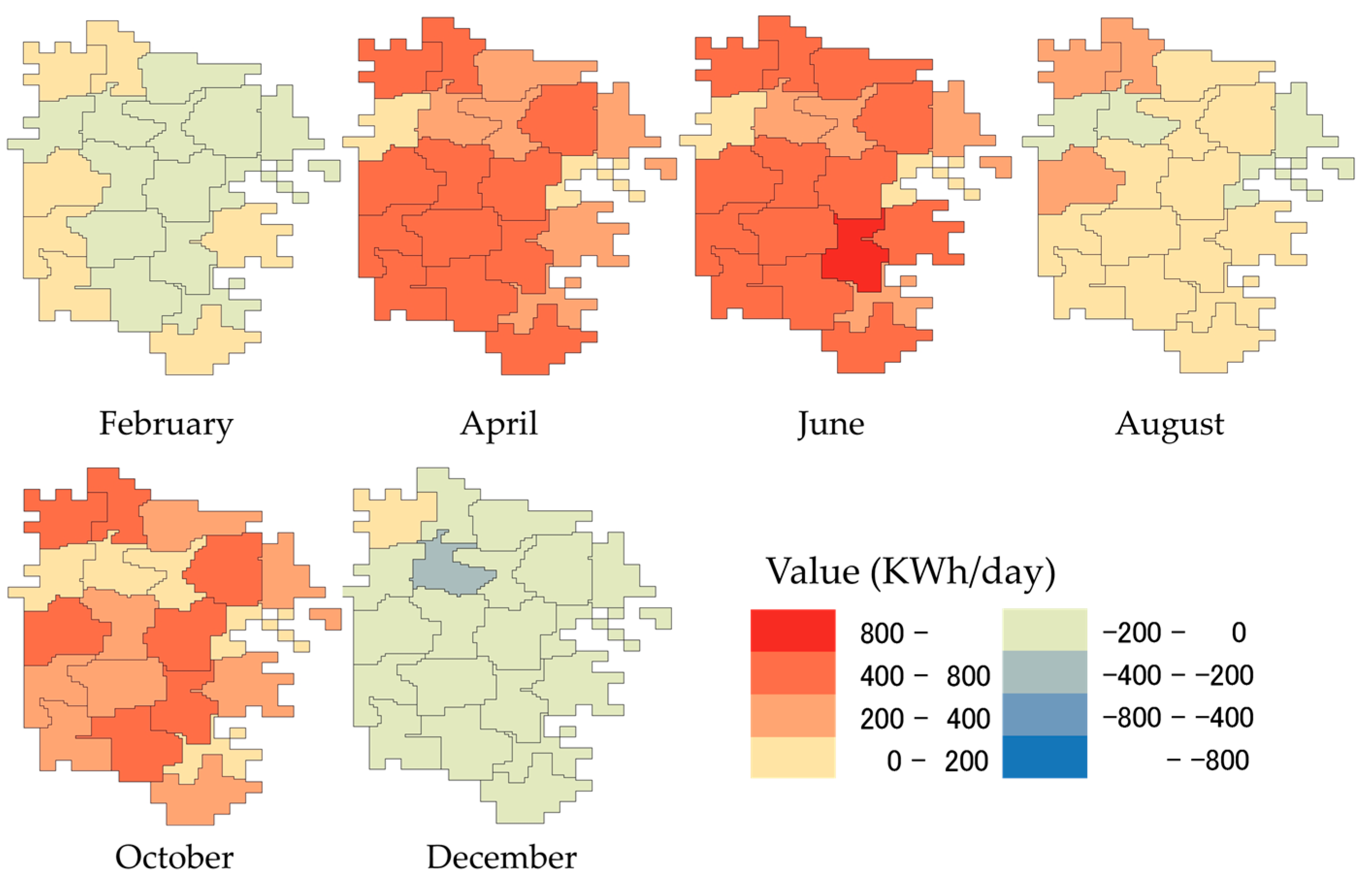
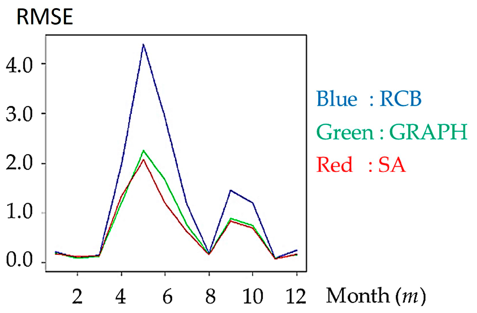
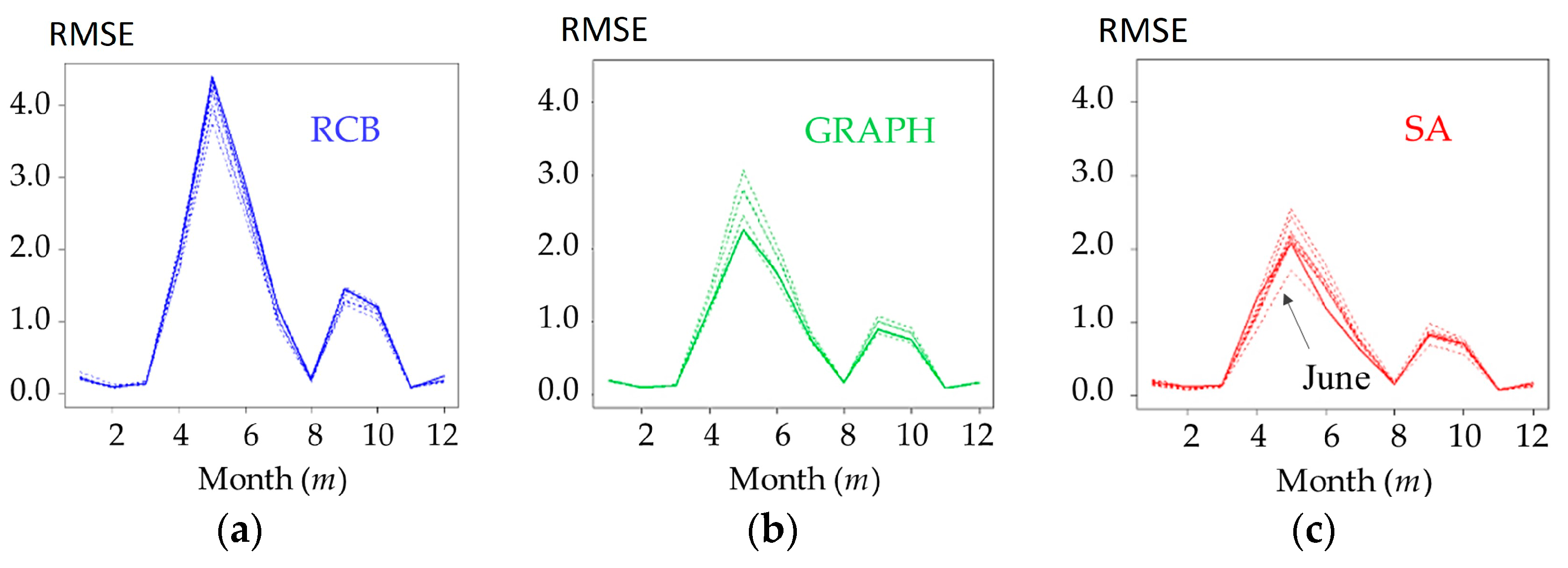
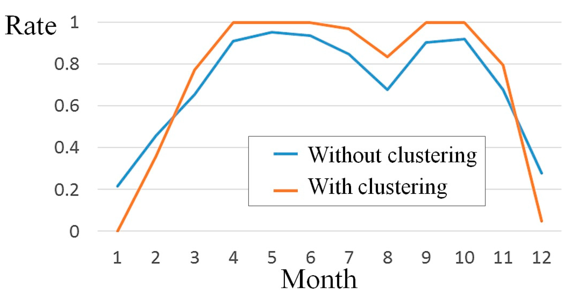
4.2. Comparison of Clustering Results

Figure 3 displays community clustering results for the six months. Note that we divide the electrical grid into 20 clusters using the RCB and GRAPH algorithms, since they are not explicitly designed to minimize the cost function in Equation (2), but rather to maintain the weighted sum of the clusters under the threshold k in Definition 1. Even so, we expect that the GRAPH algorithm minimizes the cost function when the graph is partitioned into a fixed number of clusters because the MLG algorithm’s goal is to minimize the number of edges across different clusters. The RCB clusters are almost the same through the months; based on the RCB algorithm, the same set of clusters are available in each month, which greatly increases the feasibility of community clustering.

To quantify the similarity of clusters across months, the similarity between clusters in months m (G_m) and m − 1 (G_m-1) are evaluated sequentially using the Jaccard similarity coefficient (e.g., [31]), which is formulated as follows:

$$J(G_m,G_{m-1})=\frac{\left|G_m\cap G_{m-1}\right|}{\left|G_m\cup G_{m-1}\right|}$$

(8)

J(G_m, G_m−1) approaches 1 if the two clustering results, G_m and G_m−1, are similar, and approaches 0 if they are dissimilar. Figure 4 plots the estimated Jaccard similarity coefficients. The RCB clusters in each month are quite similar, and their coefficients are around 0.95. By contrast, the GRAPH clusters indicate weaker similarity, with coefficients around 0.7 to 0.8. Thus, the RCB algorithm is more preferable in terms of the stability of the clusters, which increases the feasibility of implementation. The coefficients of the SA algorithm are moderate and highly variable.

To compare the electricity-sharing costs, circularity of clusters are compared in each month and plotted in Figure 5. Note that the cost is small if clusters are circular-shaped. The solid lines in Figure 5 denote average circularity for all of the clusters in each month, and the dashed lines denote the minimum circularity among the clusters. Based on this figure, the GRAPH algorithm provides the most circular-shaped clusters, and the GRAPH algorithm would be preferable in terms of reducing electricity-sharing costs. On the other hand, the minimum circularity of each algorithm is similar, indicating that GRAPH is the best in terms of the average sharing cost, but all three algorithms (RCB, GRAPH, and SA) are compatible in terms of the optimum electricity-sharing cost among the clusters.

Figure 6 plots the root mean squares of storage availabilities in each month. From Equation (2), it is readily verifiable that these values are equivalent to the root mean squared error (RMSE), which is a standard error statistic (e.g., [32]), quantifying the difference between the storage capacity and the surplus electricity. While the objective functions of graph partitioning (RCB/GRAPH) and meta-heuristic (SA) algorithms are different because of their basic underlying assumptions (see the beginning of Section 3), both attempt to minimize the RMSE, using Equations (3) and (6), respectively. The RCB clusters show large RMSEs (Figure 6), indicating that the RCB clusters are not preferable in terms of storage sufficiency. The SA clusters have smaller RMSEs than RCB and GRAPH. The SA clusters would, therefore, be preferable in terms of storage sufficiency. Note that GRAPH clusters also have small RMSEs, indicating that these clusters are also reasonably self-sufficient.

We have discussed cluster optimization in each month. However, due to implementation costs, using only one clustering result for all months would be desirable. Figure 7 plots RMSEs when the clustering result optimized for one month is used across all months. This figure shows that the SA clusters optimized in June minimize the RMSEs through the entire year.

The effectiveness of using a common cluster set across months is due to the time-invariance of the spatial distributions of PV panels, EVs, and households, which determines the electricity self-sufficiency. Owning to this property, desirable community clusters would be similar throughout a year. It is likely that the time-invariance holds in many other countries and regions. Applying a cluster set throughout years appears to be a reasonable approach.

Still, it is unclear how optimal these clusters are. Since clustering problems are usually difficult to solve (i.e., NP-hard), identification of “good enough” clusters is a usual concern. While we face the same difficulty, since SA asymptotically converges to the global optimum (see, Section 3.3), the monthly SA clusters must be nearly optimal in each month. Additionally, owing to the time-invariance property, which we discussed just above, optimization of the SA clusters holds even if one clustering result is applied throughout the year. Considering the high optimality and feasibility, use of one SA-based clustering result across months would be a good option. Although we subsequently focus on the cluster optimized in June, whose RMSEs are the smallest (see, Figure 7c), a similar discussion holds for the other 11 clustering results, since cluster shapes are similar across months (see, Figure 3c).

To verify the effectiveness of the June SA clusters, the storage sufficiency of the June clusters are plotted in Figure 8 and summarized in Figure 9. Interestingly, Figure 9 shows that all of the June SA clusters fulfill the self-sufficiency criteria in April, May, June, September, and October. The lack of the storage sufficiency appearing in the other months is quite small as compared with the individual grid level (i.e., negative values, which appear in Figure 8, are quite small compared to those in Figure 2). The June SA clusters, therefore, significantly increase the electricity self-sufficiency.

5. Concluding Remarks

We compared clustering algorithms, including fast or exhaustive options, in terms of electricity self-sufficient community clustering. The analysis result reveals advantages and disadvantages when using each algorithm. The RCB algorithm provides clusters that are stable across months. The GRAPH algorithm provides circular-shaped clusters with small electricity sharing cost and reasonably high self-sufficiency. The SA algorithm provides the most self-sufficient clusters. We also demonstrate that the use of the SA clusters optimized in June for all months is a sensible method in terms of both self-sufficiency and the feasibility. Our analysis takes an important first step towards designing energy sharing community clusters for the V2C system.

Still, we have many issues that must be discussed in order to effectively implement the V2C system. First, it is important to analyze the trade-off between implementation/maintenance costs and electricity self-sufficiency. This trade-off analysis would be necessary for effective implementation and operation of this system. Second, further discussion of intangible aspects is needed. How can we generate social acceptance, deliver the product to society, and design a profitable business model? To better consider these issues, some social-level experiments would be needed. Fortunately, there are a number of smart-grid initiatives and test sites in Japan (see, [19]). Conducting a social experiment in collaboration with these activities would be an important next step towards implementing the V2C system.

A deeper discussion of the local community design is also needed. The electricity sharing community might further encourage related collaborative activities, such as car sharing, event sharing, and helping neighbors on a daily basis or in an emergency. To design not only electricity sharing but also these collaborative activities, both of which can increase human well-being, we need to design the local communities with consideration for coordinating resident activities and allocating facilities (e.g., EVs and their stations). Consideration of the transportation network would also be important to encourage transportation sharing and electricity sharing by carrying batteries (which might be needed in extreme events).

Cities are not homogeneous two-dimensional (2D) systems as we implicitly assumed; rather, urban physical form is normally heterogeneous and has 3–4 essential dimensions determined by physical characteristics, such as topography, 3D urban street canyons, and microclimate (see, [33,34,35]). Residents and their behavioral patterns are also heterogeneous. Integration of net-zero community clustering with 3D urban modeling or scenario analysis would be an exciting step toward smart and sustainable development.

References

1. Ackermann, T.; Andersson, G.; Soder, L. Distributed generation: A definition. Electr. Power Syst. Res. 2001, 57, 195–204. [Google Scholar] [CrossRef]
2. Wolsink, M. The research agenda on social acceptance of distributed generation in smart grids: Renewable as common pool resources. Renew. Sustain. Energy Rev. 2012, 16, 822–835. [Google Scholar] [CrossRef]
3. Hirabayashi, Y.; Mahendran, R.; Koirala, S.; Konoshima, L.; Yamazaki, D.; Watanabe, S.; Kim, H.; Kanae, S. Global flood risk under climate change. Nat. Clim. Chang. 2013, 3, 816–821. [Google Scholar] [CrossRef]
4. Huang, J.; Jiang, C.; Xu, R. A review on distributed energy resources and MicroGrid. Renew. Sustain. Energy Rev. 2008, 12, 2472–2483. [Google Scholar]
5. Nichols, D.K.; Stevens, J.; Lasseter, R. Validation of the CERTS MicroGrid concept the CEC/CERTS MicroGrid testbed. IEEE Power Eng. Soc. Gen. Meet. 2006. [Google Scholar] [CrossRef]
6. Branker, K.; Pathak, M.J.M.; Pearce, J.M. A review of solar photovoltaic levelized cost of electricity. Renew. Sustain. Energy Rev. 2011, 15, 4470–4482. [Google Scholar] [CrossRef]
7. Kempton, W.; Tomic, J. Vehicle-to-grid power fundamentals: Calculating capacity and net revenue. J. Power Sour. 2005, 144, 268–279. [Google Scholar] [CrossRef]
8. Lund, H.; Kempton, W. Integration of renewable energy into the transport and electricity sectors through V2G. Energy Policy 2008, 36, 3578–3587. [Google Scholar] [CrossRef]
9. Srivastava, A.K.; Annabathina, B.; Kamalasadan, S. The challenges and policy options for integrating plug-in hybrid electric vehicle into the electric grid. Electr. J. 2010, 23, 83–91. [Google Scholar] [CrossRef]
10. Green, R.C.; Wang, L.; Alam, M. The impact of plug-in hybrid electric vehicles on distribution networks: A review and outlook. Renew. Sustain. Energy Rev. 2011, 15, 544–553. [Google Scholar] [CrossRef]
11. Yamagata, Y.; Seya, H. Spatial electricity sharing system for making city more resilient against X-events. Innov. Supply Chain Manag. 2013, 7, 75–82. [Google Scholar] [CrossRef]
12. Yamagata, Y.; Seya, H. Proposal for a local electricity-sharing system: A case study of Yokohama city, Japan. IET Intell. Transp. Syst. 2015, 9, 38–49. [Google Scholar] [CrossRef]
13. Arizumi, N.; Minami, K.; Tanjo, T.; Maruyama, H.; Murakami, D.; Yamagata, Y. A first step towards resilient graph partitioning for electrical grids. In Proceedings of the 7th International Conference on Information and Automation for Sustainability, Colombo, Sri Lanka, 22–24 December 2014; pp. 1–6.
14. Peterson, S.B.; Whitacre, J.F.; Apt, J. The economics of using plug-in hybrid electric vehicle battery packs for grid storage. J. Power Sour. 2010, 195, 2377–2384. [Google Scholar] [CrossRef]
15. Zhang, Q.; Tezuka, T.; Ishihara, K.N.; Mclellan, B.C. Integration of PV power into future low-carbon smart electricity systems with EV and HP in Kansai Area, Japan. Renew. Energy 2012, 44, 99–108. [Google Scholar] [CrossRef]
16. Nissan Motor Co., Ltd. Available online: http://www.nissan.co.jp/EN/ (accessed on 13 July 2016).
17. World Energy Council. Available online: https://www.worldenergy.org (accessed on 13 July 2016).
18. Next Generation Vehicle Promotion Center. Available online: http://www.cev-pc.or.jp/english/ (accessed on 13 July 2016).
19. Ling, A.P.A.; Sugihara, K.; Mukaidono, M. The Japanese smart grid initiatives, investments, and collaborations. Int. J. Adv. Comput. Sci. Appl. 2012, 3, 44–54. [Google Scholar]
20. Automobile Inspection and Registration Information Association. Available online: https://www.airia.or.jp/ (accessed on 13 July 2016). (In Japanese)
21. Japan Photovoltaic Energy Association. Available online: http://www.jpea.gr.jp/en/greeting/index.html (accessed on 13 July 2016).
22. Berger, M.J.; Bokhari, S.H. A partitioning strategy for nonuniform problems on multiprocessors. Comput. IEEE Trans. 1987, 36, 570–580. [Google Scholar] [CrossRef]
23. Bui, T.N.; Jones, C. A heuristic for reducing fill-in in sparse matrix factorization. Proc. Parallel Process. Sci. Comput. 1993, 1, 445–452. [Google Scholar]
24. Hendrickson, B.; Leland, R. Multidimensional Spectral Load Balancing. U.S. Patent 5,587,922, 24 December 1996. [Google Scholar]
25. Karypis, G.; Kumar, V. Metis-Unstructured Graph Partitioning and Sparse Matrix Ordering System, 2nd ed.; University of Minnesota: Mineapolis, MN, USA, 1995. [Google Scholar]
26. Kirkpatrick, S.; Gelatt, C.D., Jr.; Vecchi, M.P. Optimization by simulated annealing. Science 1983, 220, 671–680. [Google Scholar] [CrossRef] [PubMed]
27. Openshaw, S. Optimal zoning systems for spatial interaction models. Environ. Plan. A 1977, 9, 169–184. [Google Scholar] [CrossRef]
28. Martin, D. Extending the automated zoning procedure to reconcile incompatible zoning systems. Int. J. Geogr. Inf. Sci. 2003, 17, 181–196. [Google Scholar] [CrossRef]
29. The Multi-Agent Transport Simulation MATSim; Horni, A.; Nagel, K.; Axhausen, K.W. (Eds.) Ubiquity: London, UK, 2016.
30. Itagaki, A.; Okamura, H.; Yamada, M. Preparation of meteorological data set throughout Japan for suitable design of PV systems. In Proceedings of the 3rd World Conference on Photovoltaic Energy Conversion, Osaka, Japan, 18 May 2003; pp. 2074–2077.
31. Seifoddini, H.; Djassemi, M. The production data-based similarity coefficient versus Jaccard’s similarity coefficient. Comput. Ind. Eng. 1991, 21, 263–266. [Google Scholar] [CrossRef]
32. Bishop, C. Pattern Recognition and Machine Learning; Springer-Verlag: New York, NY, USA, 2007. [Google Scholar]
33. Quan, S.J.; Li, Q.; Augenbroe, G.; Brown, J.; Yang, P.P.J. Urban data and building energy modeling: A GIS-based urban building energy modeling system using the urban-EPC engine. Plan. Support Syst. Smart Cities 2015, 24, 447–469. [Google Scholar]
34. Li, Z.; Quan, S.J.; Yang, P.P.J. Energy performance simulation for planning a low carbon neighborhood urban district: A case study in Macau. Habitat Int. 2016, 53, 206–214. [Google Scholar] [CrossRef]
35. Yamagata, Y.; Murakami, D.; Yoshida, T.; Seya, H.; Kuroda, S. Value of urban views in a bay city: Hedonic analysis with the spatial multilevel additive regression (SMAR) model. Landsc. Urban Plan. 2016, 151, 89–102. [Google Scholar] [CrossRef]
Figure 1. Number of vehicles owned (left: EV; middle: hybrid EV; source: [20]) and production of PV modules for domestic use (right) in Japan (source: [21]).
Energies 09 00543 g001
Figure 2. Estimated storage availability for six months in each 250-m grid.
Energies 09 00543 g002
Figure 3. Community clustering results of (a) RCB; (b) GRAPH; and (c) SA algorithms.
Energies 09 00543 g003
Figure 4. Jaccard’s similarity coefficients in each month. Large coefficients for RCB suggest that shapes of the RCB clusters are similar across months, while the small coefficients for GRAPH suggest that the opposite is true for the GRAPH clusters.
Energies 09 00543 g004
Figure 5. Circularity in each month. The solid lines denote average circularity for all of the clusters in each month, and the dashed lines denote the minimum circularity among the clusters.
Energies 09 00543 g005
Figure 6. RMSEs (storage capacity vs. PV electricity) of the clusters optimized in each month.
Energies 09 00543 g006
Figure 7. RMSEs (storage capacity vs. PV electricity) of the month-wise optimized clusters (solid lines) and of the clusters from a given month applied to all months (dashed lines). (ac) denote results of RCB, GRAPH, and SA algorithms, respectively.
Energies 09 00543 g007
Figure 8. Storage sufficiency (per 250-m grids) of the SA clusters optimized in June.
Energies 09 00543 g008
Figure 9. Rate of self-sufficient grids. Blue indicates the rates of grids whose storage sufficiency is positive, and is calculated as [the number of grids with positive storage-sufficiency]/6,687. Red indicates the rates of grids that are in community clusters with positive storage sufficiency, and is calculated as [the number of grids in a cluster, Gi, with positive storage-sufficiency]/6,687. The total number of grids is 6,687.
Energies 09 00543 g009