1. Introduction
The traffic volume towards data-centers (DCs) has been constantly increasing [
1] during the last ten years. This is due to the fact that the “cloud” paradigm has gained importance in the Internet. As an example, different big players (like Google, Amazon, Dropbox) are offering cloud storage, thus allowing both single users and whole organizations to move data from/to the cloud. In this context, the DC architecture and the management of the servers inside the DC has gained a significant role. In particular, service providers managing DCs are facing two contrasting issues: (i) the requests from users need to be served in a reasonable bounded delay; and (ii) the energy costs for managing the DC have to be reduced. In the literature, both these issues have been extensively studied (e.g., [
2,
3]), focusing both on intra-DC solutions (
i.e., involving the servers inside a single DC), or inter-DC ones (
i.e., considering as a whole the set of DCs managed by the cloud provider).
When the objective functions like the minimization of delay or energy are pursued, different power states are applied to the servers of the DC. More in depth, a subset of servers may be even put in sleep mode (SM) to maximize the electricity savings [
4]. Although the benefits from changing the server power state in a DC are clear (
i.e., electricity cost reduction or performance improvement), the implications of applying such policies in real DC implementations have been only marginally studied. In this context, several question arise, such as: What is the impact of power management policies on the lifetime on servers? Is it possible to define a model for the lifetime of a server subject to power state changes? Specifically, the lifetime is defined as the amount of time between one failure and the following one [
5]. When the server lifetime is decreased, its failure rate is increased, thus negatively impacting the user’s quality of experience (QoE). On the other hand, the related costs incurred for fixing the failed servers may also erode the electricity saved by the DC service provider. The scope of this work is therefore to investigate this impact by proposing a primary model of the lifetime for a set of servers subject to power state changes. Moreover, we evaluate the proposed model in different case-studies driven by energy minimization and/or delay minimization goals. Our results indicate that the server’s lifetime should be carefully considered when power management policies are applied—
i.e., how and when to apply a server power state in a DC. We believe that this work could pave a new way to further investigation. In particular, we show that the lifetime is also heavily influenced by the hardware (HW) parameters used to build the servers, and therefore a careful measurement of these parameters in a working scenario is of mandatory importance. Additionally, we believe that new power management algorithms considering user performance, energy minimization, and server lifetime should be developed. We leave both these aspects for future work. The rest of the paper is organized as follows. Related works are presented in
Section 2. The main effects related to temperature which impact server lifetime are summarized in
Section 3.
Section 4 then presents our model for estimating the server lifetime.
Section 5 reports the scenario adopted to evaluate our model. Results, obtained from a realistic case study, are detailed in
Section 6. Finally,
Section 7 reports the conclusions and the future work.
2. Related Work
The closest paper to this work is [
5], in which authors propose a simple model for evaluating the impact of energy-aware policies on the lifetime of cellular and backbone network devices. However, the research in cellular and backbone devices is generally different than the one developed for the server case. For example, the total power consumption of network devices hardly scales with the load [
6], while the server machines tend to be more power proportional. In this work, we go three steps further by:
- (i)
focusing on a DC scenario;
- (ii)
proposing a completely new model that accounts for transitions among different power states (in other words, not only a SM and full power like in [
5]);
- (iii)
evaluating the impact of applying a management policy for the servers in a DC.
We believe that these improvements are of fundamental importance for understanding the energy, quality of service (QoS), and lifetime trade-off in cloud DCs. Our model is rather general, and, to the best of our knowledge, is representative for the server case. However, the physical phenomena affecting the lifetime of microelectronics components (like chip packages) are common in both backbone, cellular, and server devices. Moreover, we also add that current trends in backbone and cellular network devices foresee the exploitation of commodity HW (thanks to the introduction of new paradigms like Software Defined Networking [
7] and Network Function Virtualization [
8]). This HW will likely operate like server machines, so we envision the application of the model presented in this paper even in these cases.
In general, the variation of power (and consequently of temperature), has an impact on device lifetime. More in depth, in [
9] authors report temperature measurements of disks, memories, and components in DCs, showing that the largest impact on failure rates is due to the variation of temperature rather than its increase. Moreover, the authors show that the failure rate of HW components is linear with temperature rather than exponential. Finally, a linear dependency of power with temperature is shown. In our work, we have considered all these aspects. In particular, we have proposed a failure model taking into account power variation. Additionally, we have assumed that the failure rate increases linearly with temperature.
The management of jobs between different DCs may pursue different goals. Specifically, in [
10] authors exploit the variation of electricity prices in order to reduce the associated costs in DCs. More in depth, the servers are geographically distributed among different zones. In this scenario, the job requests are moved among the different DCs in order to exploit the DC(s) experiencing the lowest electricity prices. Additionally, in [
11] authors take into account capacity provisioning in cloud DCs with the goal of reducing the brown energy—
i.e., energy generated from non-renewable sources. Finally, in [
12] authors consider the consumption of water for dispatching jobs in geographical DCs. All of these works do not consider the impact of the proposed policies on the failure rate of the servers in each DC. In contrast to them, here we focus on the impact of a policy to manage jobs in cloud DCs on server lifetime.
Reducing power consumption in a single DC is a hot topic. In the past years, different works have targeted this problem (for example, [
13] for a detailed survey). In particular, Beloglazov and Buyya [
4] have considered the consolidation of virtual machines (VMs) in order to bring substantial energy savings while ensuring reliable QoS. Additionally, Heller
et al. [
14] and Fanf
et al. [
15] targeted the energy reduction of the networking infrastructure. All these works prove the efficacy and the efficiency of these solutions in terms of energy, without considering the impact on the failure rate due to power state transitions. Our work is instead devoted to the investigation of the server lifetime in each DC of the cloud provider. Although there are several objectives (
i.e., user QoE, energy inside the DC, energy among a set of DCs, electricity costs, brown energy, water consumption) that can be pursued during the management of the DC, we believe that the impact of failure rate should be also controlled. In the next section, we therefore investigate the main physical phenomena affecting the server failure rate and consequently its lifetime.
3. Physical Factors Affecting Server Lifetime
A first order model to compute the failure rate
of a device given its temperature
T is the Arrhenius law [
16]:
where
is the failure rate estimated assuming a very high temperature,
is the activation energy (
i.e., the minimum energy needed to activate the failure variation), and
K is the Boltzmann constant. Interestingly, when the temperature is decreased, the failure rate is also decreased. Although more detailed models have been proposed in the literature (e.g., [
17]) all of them predict a decrease in the failure rate when the temperature is reduced. This means that if the reduction of temperature was the only effect taken under consideration, keeping the server in the lower power states for the longest amount of time would be of benefit for its lifetime. However, we stress that Equation (
1) is just a first-order approximation. For example, according to [
9], failure rates exhibit a linear dependency with temperature (rather than exponential). Therefore, we will consider this aspect when defining a model for the server failure rate.
In the following, we consider the second effect impacting the lifetime—
i.e., the temperature variation. In this case, a device may suffer strain and fatigue when temperature conditions change, especially when this happens in a cyclical fashion (
i.e., from one temperature to another). The Coffin–Manson model [
18] describes the effects of material fatigue caused by cyclical thermal stress. The predicted failure rate
due to the thermal cycling effect is then expressed as:
where
is the frequency of thermal cycling and
is the estimated failure rate. The term
is the number of cycles to failure, and it is commonly denoted as:
where Δ
T is the temperature variation of the cycle,
is the maximum admissible temperature variation without a variation in the failure rate,
is a constant material dependent, and
q is the Coffin–Manson exponent. From this model, we can clearly see that the more often the server experiences a temperature variation, the higher its failure rate will be. In the following, we therefore build a model to capture this effect and also to consider the impact of temperature decrease reported in Equation (
1).
4. Server Lifetime Model
We first consider the model for a single server, then we detail the steps to extend this model to the whole DC under consideration. In particular, we assume that the total period of time under consideration is denoted as T, divided in time slots. Each time slot is denoted by a duration . Moreover, we assume —i.e., the time needed to perform transitions is negligible with respect to the time slot duration. The power consumption of the server at time slot k is denoted as , which is equal to 0 if the server is put in SM, or a value between and if the server is active. takes into account the whole power consumed by the server. This term scales linearly with the server load—i.e., it is for the minimum load and may be increased up to for the maximum load. When the load is equal to zero, we assume that the server is in SM—i.e., .
We then consider the impact of power state transitions. Specifically, when the server load is varied across two consecutive time slots, a power state change of the whole server is triggered. Let us denote as the absolute difference of the power consumption at k-th time slot and the one at the -th time slot—i.e., . Moreover, let us denote as the maximum difference in power consumption for active states—i.e., .
We then introduce the binary variables used in our model. In particular, we denote
as the SM state setting at time
k:
Moreover, we introduce the binary variable
, which takes value equal to one if the server has experienced a SM-active transition between the current time slot and the previous one, zero otherwise:
Note that an alternative definition of is , where ⊕ is the exclusive disjunction (XOR) operator.
Finally, we introduce binary variable
, which takes value one if the server has experienced an active power transition between the current time slot and the previous one, zero otherwise.
We then consider a metric called acceleration factor (AF), introduced in [
5]. The AF is denoted as the ratio between the current failure rate (
i.e., by applying power management policies) and a fixed reference failure rate (which we assume to be the case in which the server is always kept at full power). Therefore, the AF is simply a normalized failure rate. The failure rate can be obtained by multiplying the AF for the reference failure rate. Specifically, the AF takes into account the lifetime decrease/increase introduced by energy-aware policies. In particular, if the AF is lower than one, the lifetime is increased compared to a full power situation. On the contrary, if the AF is higher than one, the lifetime is decreased. We refer the reader to [
5] for a detailed explanation of this metric. In this work, we will decompose the AF in different sub-terms, due to the following effects:
- (i)
SM state setting;
- (ii)
active power setting;
- (iii)
power state transition between the active states (not involving SM);
- (iv)
power state transitions between an active state and a SM state.
The total
is the sum of the AF due to power states
and the AF due to transitions
:
In particular, depends solely on the amount of time spent in each power state and the AF of that state. At the same time, depends solely on the frequency of power state transitions and the penalties for the transitions.
More in depth,
can be decomposed in the following way:
where
accounts for the AF in SM over the period
T, while
takes under consideration the AF of active transitions over the period
T. In particular,
can be expressed as follows:
where
is the AF of the server in SM (without considering the time period). Thus,
is the AF in SM, weighed by the amount of time the server spends in SM. Focusing on
, we can express it in the following way:
In particular, we have considered that the AF due to active state is extracted by interpolation between the minimum amount of power
and the maximum one
. The intuition suggests in fact that the server temperature is lower when the power is decreased. Therefore, we also expect a lower AF. Additionally, we assume that the AF at maximum power is equal to one. (Equation (
10) may also be rewritten to include Equation (
9), but we prefer to keep both of them in order to evaluate them separately in the results section.) The reasons for choosing a linear dependency of AF with power are as follows:
- (i)
the power tends to increase linearly with temperature (as reported by [
9]);
- (ii)
the exponential model presented in Equation (
1) tends to over-estimate the failure rate increase with temperature.
Therefore, a more realistic model is the linear one.
In the next step, we consider the AF due to transitions, expressed as:
where
is the AF due to an SM-active state transitions, and
is the AF due to transition between active power states. In particular, we define
as:
where
is a weight parameter for the frequency of SM-active transitions
. This parameter depends solely on the HW used to build the device. Additionally, we define
as:
where
W is a scale parameter (lower than 1),
is the frequency weight for a variation of power equal to
, and
is the frequency of transitions between the active states. The parameter
W is inserted since we expect a lower impact on failure rates when variations among active states are performed, comparing to the case in which transitions involve SM.
Thus, we can see that the server AF is governed by four types of parameters:
- (i)
, , and W, which depend only on the HW used to build the device;
- (ii)
and , which are instead related to how long and how frequent SM is set;
- (iii)
, which is governed by the transitions between power states; and
- (iv)
T, which is the total period of time under consideration.
Although the HW parameters are fixed given the server, it is possible to play with the other variables, which are instead linked to the power state transitions, the power state duration, and the total period of time under consideration. Note that in this work we have considered the server as a whole by defining a model for the complete server. The application of our model to single server components is a future work. Clearly, there are components that are critical for the life of the entire server—
i.e., if one of these components fails, then the server will not able to serve traffic. These components include the memory, the CPU, and the hard disk. Therefore, in order to estimate the HW parameters of our model, one can concentrate on the single components and then extract:
- (i)
the failure rate in each power state;
- (ii)
the number of cycles to failure.
Then, by following the procedure reported in [
5], it is possible to estimate the HW parameters for the single components. Clearly, the total server AF can be defined as the average of the AF of the single components or alternatively another function—e.g., the maximum AF.
Up to this point, we have focused on the single server. Without loss of generality, we can extend the AF to the whole set of servers of the DC. More formally, let us denote with
D the set of servers of the DC, whose cardinality is
.
is the AF of
w-th server, which is defined by Equation (
7). Then, we can express the average DC AF as:
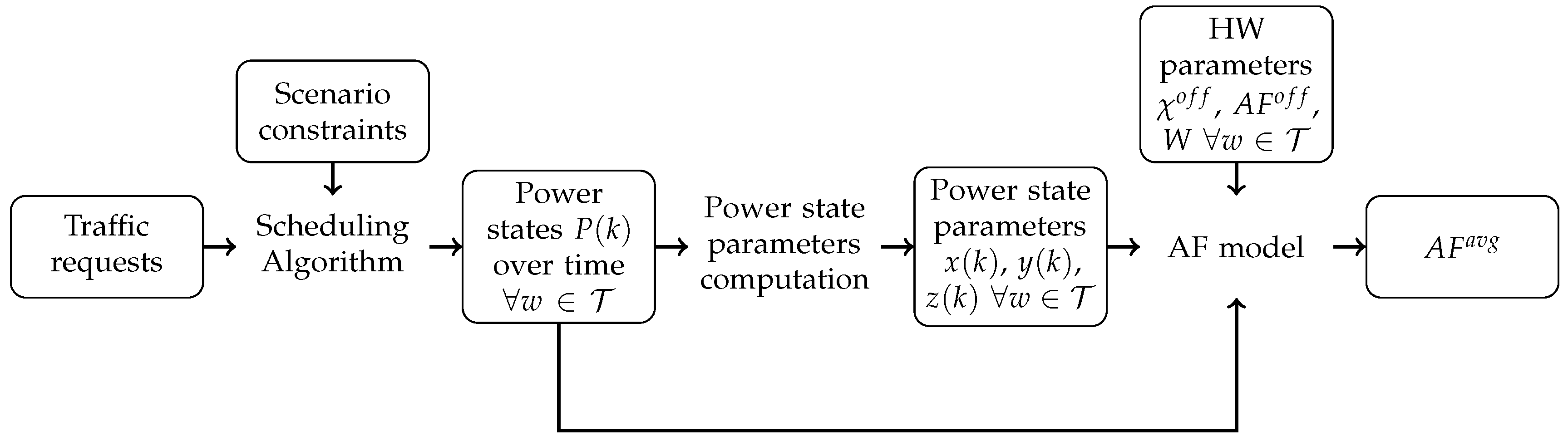
Figure 1 reports the main steps to obtain the
for a given DC. In particular, we start from traffic requests from users, and from different scenario constraints (like the number of servers and server capacity). Then, we run a scheduling algorithm to associate each request to the server. Given the request–server associations, we can estimate the server’s power consumption for each time slot
k. Then, we compute variables
,
, and
for each server. We then plug these variables, together with the power state
and the HW parameters
,
, and
W in the AF model of Equation (
14) in order to compute the average DC
.
Table 1 reports the main notation introduced so far.
6. Performance Evaluation
We first consider the number of power state changes and their duration. Unless otherwise specified, we set a value of
V equal to one for the algorithm. This value is a trade-off between delay minimization (
) and energy reduction (
). Moreover, we consider a time period
T equal to 750 h. We first focus on the transition between active power and SM, as it is the most critical one in terms of AF increase (and consequently lifetime reduction).
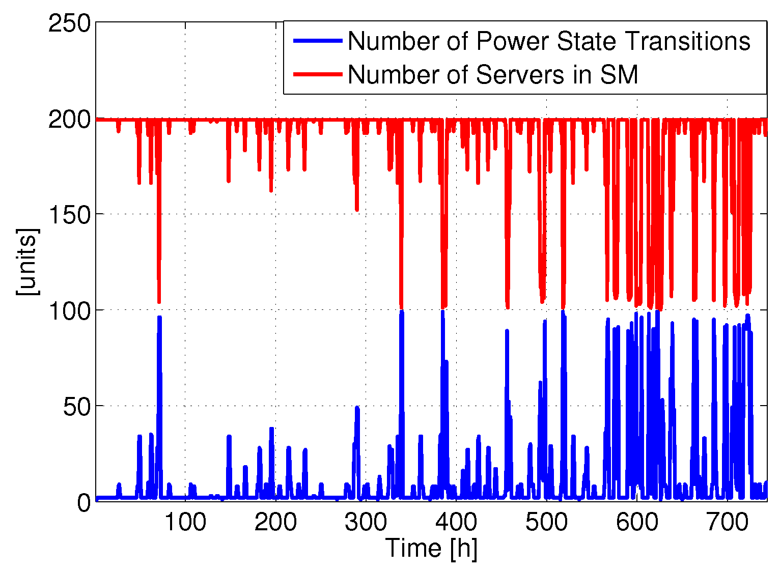
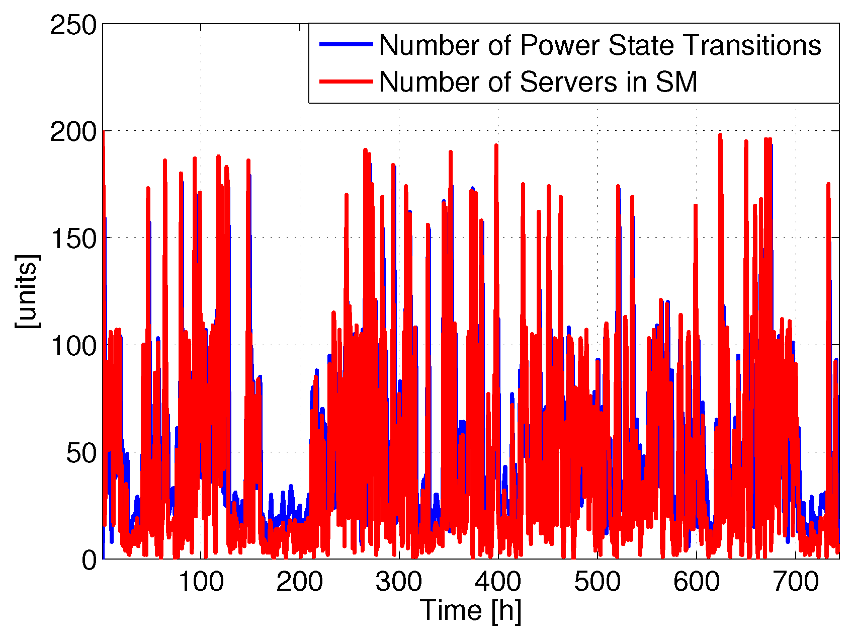
Figure 2 reports the number of power state changes involving SM and the total number of servers in SM for a single DC (the same analysis repeated on the other DCs produced similar results). Clearly, the total number of servers in SM varies over time without any daily periodicity, since the requests arrive in a random order, due to the fact that the users are spread around the world. Therefore, there is not a clear zone where traffic is low (e.g., at night). Hence, the number of servers in SM frequently changes with time, and consequently also the number of power state transitions. For example, it is possible to put most of the servers in SM at time 398 h, while shortly after they are all active. This behavior introduces a lot of transitions, which we expect to impact the lifetime.
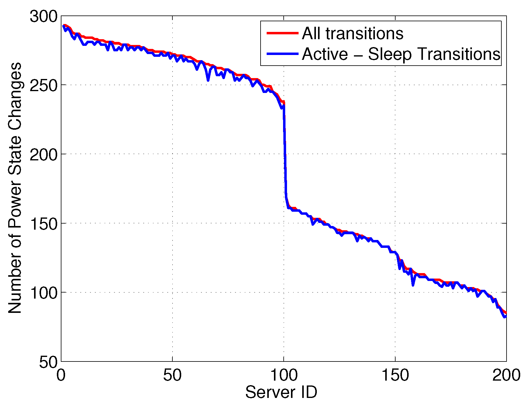
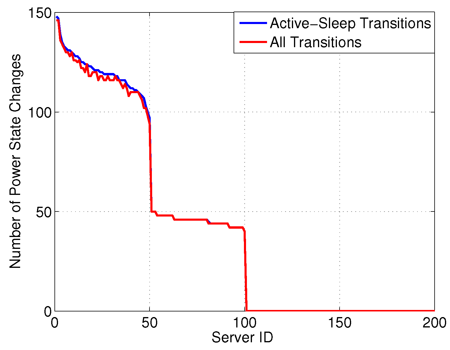
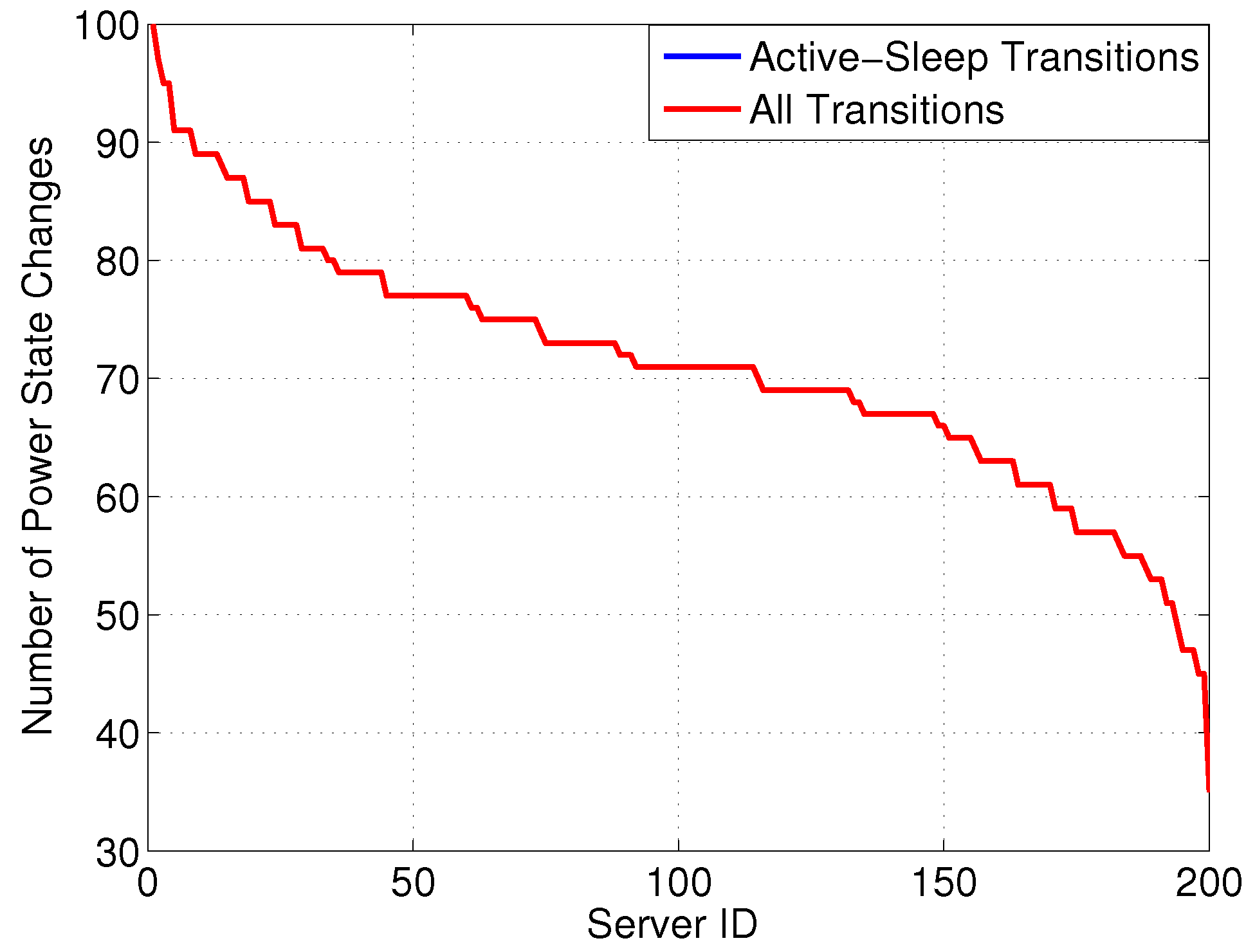
To give more insight,
Figure 3 reports the number of state changes
versus server ID, differentiating between: (i) all transitions and (ii) transitions involving a SM state. Interestingly, although the server can exploit power proportional states, most power states are either in SM or at full power, resulting in the majority of state changes involving a transition between these two states. Moreover, we can see that more than 50% of servers are experiencing quite a lot of transitions—
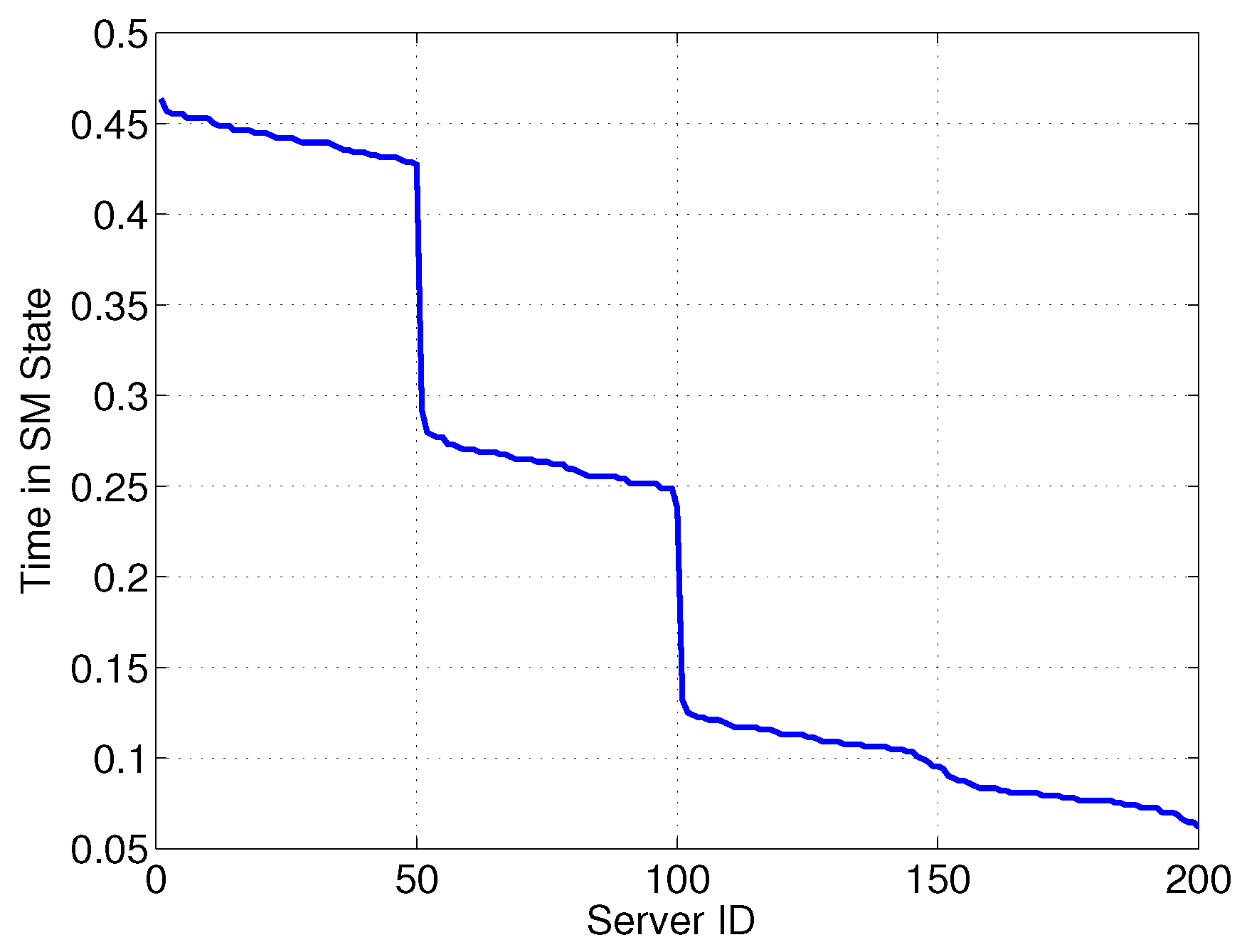
i.e., more than 200 over 750 h, which corresponds to more than 6.5 transitions per day. Additionally,
Figure 4 reports the time in SM (normalized to
T)
versus server ID. We can see that more than 50% of servers are in SM for less than 15% of the time, in order to reduce the delay for requests.
We then apply our lifetime model to the DC taken under consideration. In particular, we incrementally compute
,
,
,
,
for each time period
(
i.e., from
to
) for each server. Unless otherwise specified, we assume that the servers have the same HW components. Therefore,
,
, and
W are the same for all the servers. In particular, we initially set
,
(cycles/h), and
. The reasons for these settings are as follows:
- (i)
we consider a gain in the lifetime when the device is put in SM (or the active power is reduced);
- (ii)
we tend to penalize power state transitions involving SM;
- (iii)
we assume that the penalties of active power state transitions are much lower compared to the active-SM penalty.
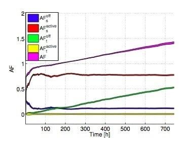
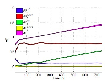
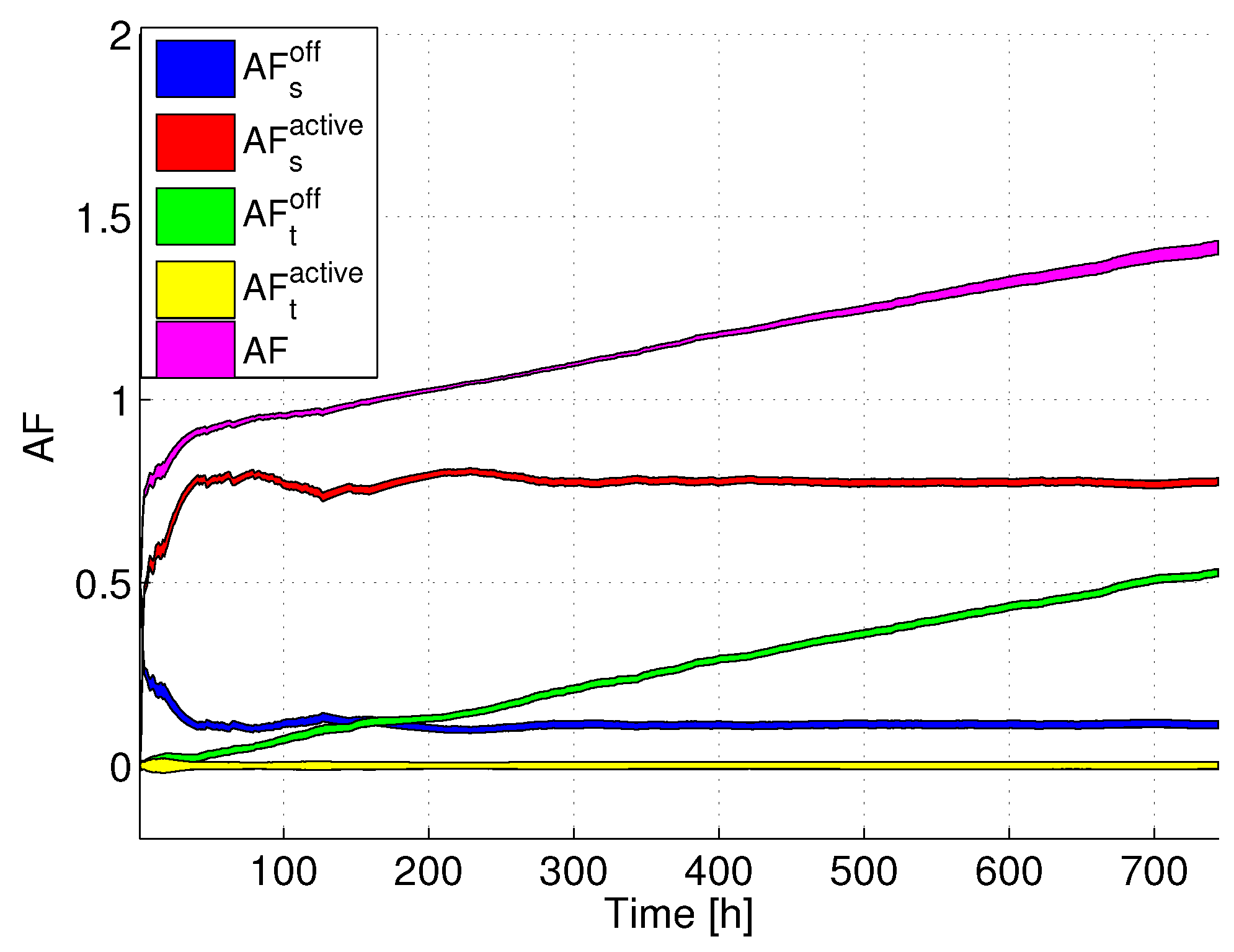
Figure 5 reports
,
,
,
,
versus time. The colored areas represent confidence intervals (assuming a 95% confidence level), computed over the whole set of servers belonging to the DC. Interestingly, we can clearly see that the total AF increases with time, passing from values lower than 1 to more than 1.4, meaning that at the end of the considered time period, the lifetime has been reduced by more than 40% compared to the case in which the servers always work at full power. Looking more in detail at the AF components, we can see that both
and
are lower than 1, meaning that their contribution tends to increase the lifetime. In particular,
is lower than one since the server is not always at full power. Additionally,
is much lower than
, due to the fact that SM is not set for all time periods, and
is lower than the AF at full power (which is equal to 1). On the contrary, the negative effect on the total AF is brought by the transitions. Although
is almost close to 0 (due to the fact that there are few transitions between active power states),
notably increases with time, due to the fact that active-SM transitions are accumulated in the DC. In the long term,
becomes the predominant term in the AF, thus bringing to a lifetime decrease with respect to the reference case, in which the servers are always at full power.
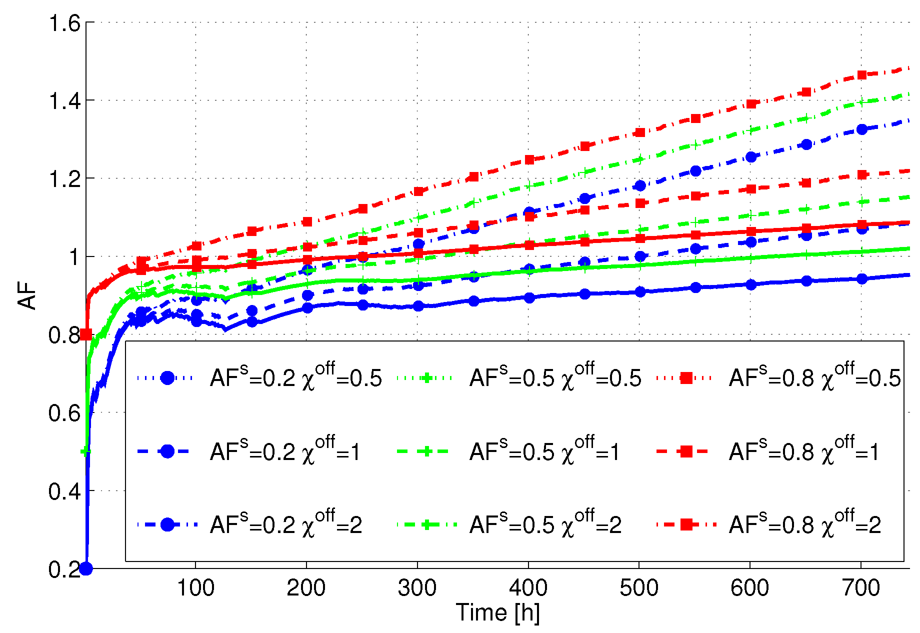
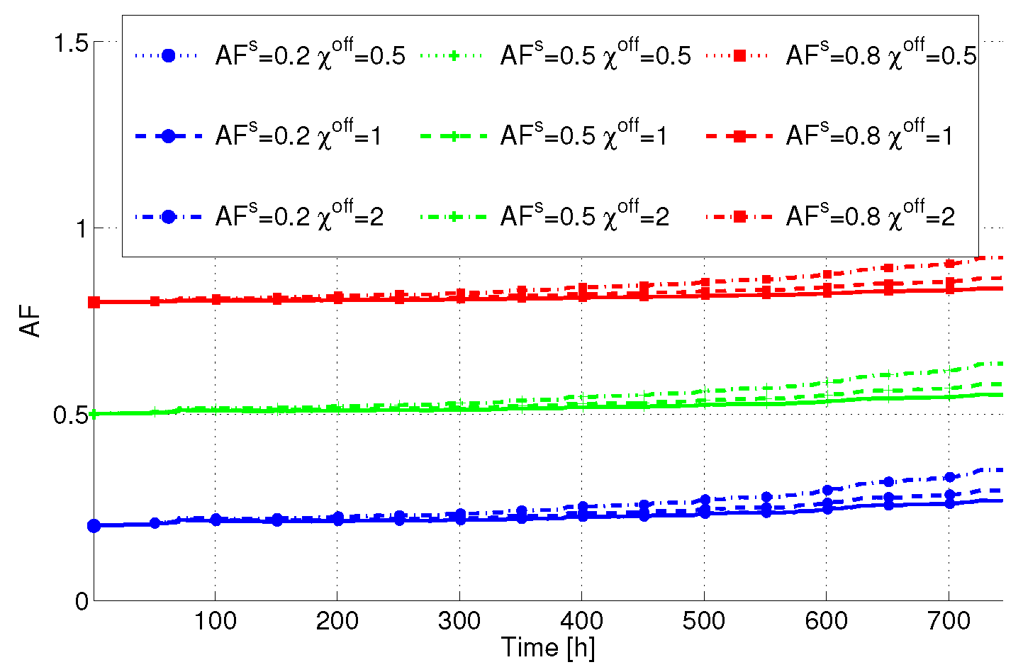
In the following step, we consider the variation of the HW parameters
and
.
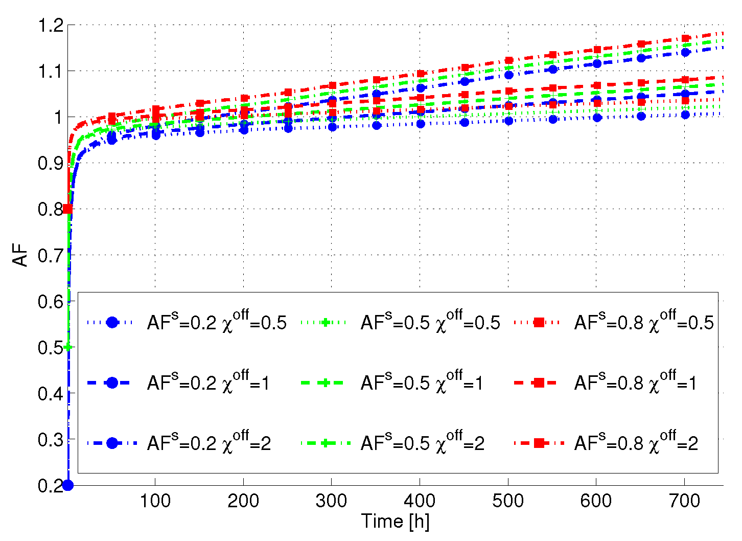
Figure 6 reports the AF
versus time averaged over the servers in the DC. Interestingly, the lower is
, the lower is also the total AF. This is due to the fact that different servers are put in SM, and consequently their AF tends to decrease when
is decreased. However, we can see that
plays a crucial role in determining the final AF. In particular, the higher
is, the higher the term in the AF due to power state variations is also. Consequently, the final AF tends to be higher than one, resulting in a lifetime decrease. From this figure, we can clearly see that lifetime-aware servers (
i.e., devices built with low
and low
) tend to limit this decrease, despite the fact that different power state transitions take place.
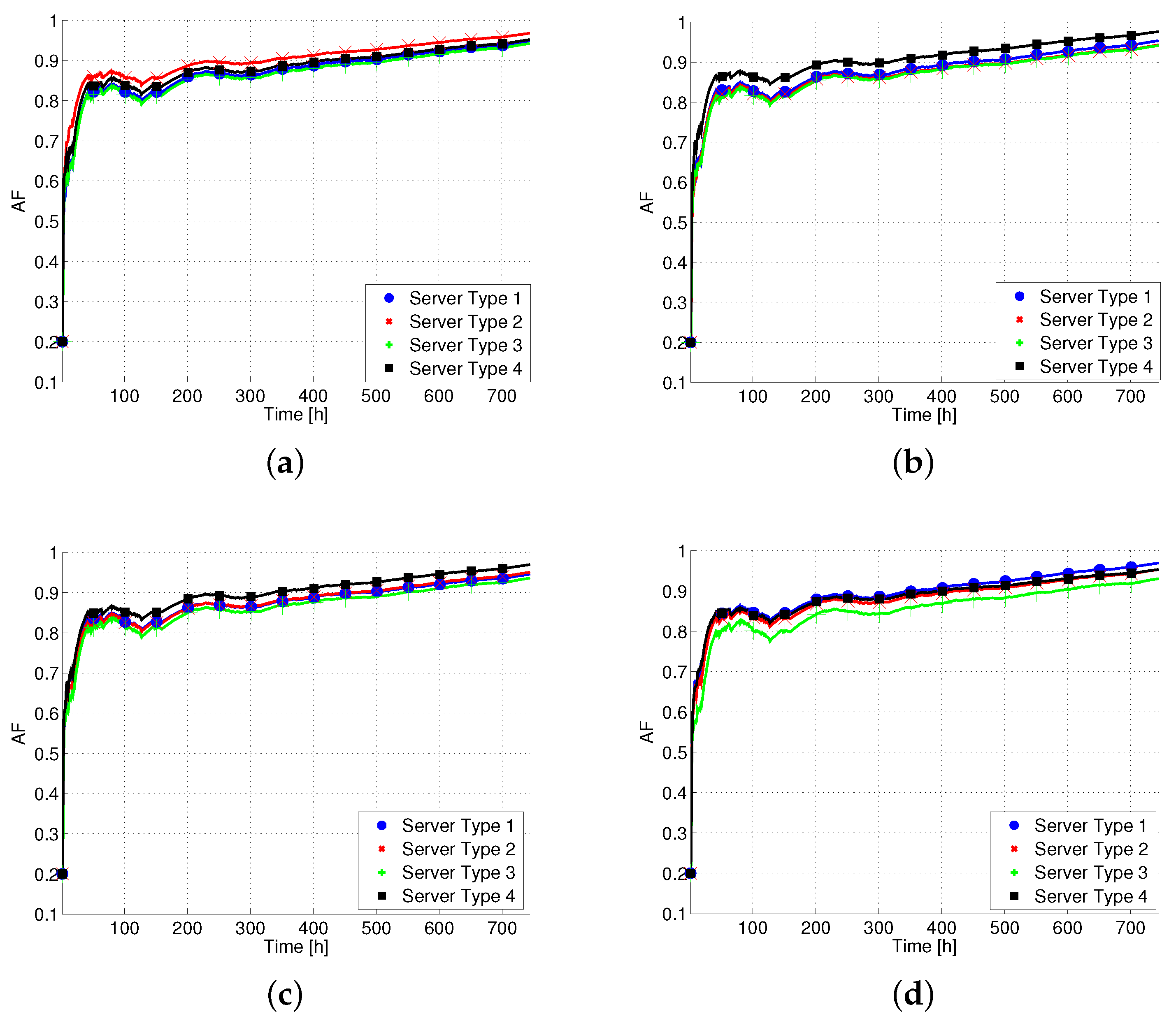
To give more insight, we have computed the AF
versus time by differentiating between the different DCs and the different server types, as reported in
Figure 7. We recall that each server type is characterized by a maximum power consumption, an idle power consumption, and a CPU speed. In particular, we can see that the AF exhibits minor variations across the DCs and the server types, suggesting that the pattern for power state transitions and power state setting is similar between them.
In the following, we consider the impact of setting a delay minimization objective or an energy reduction strategy in the algorithm by changing the values of the V parameter.
6.1. Delay Minimization Impact
We first consider the case in which
—
i.e., the delay tends to be minimized.
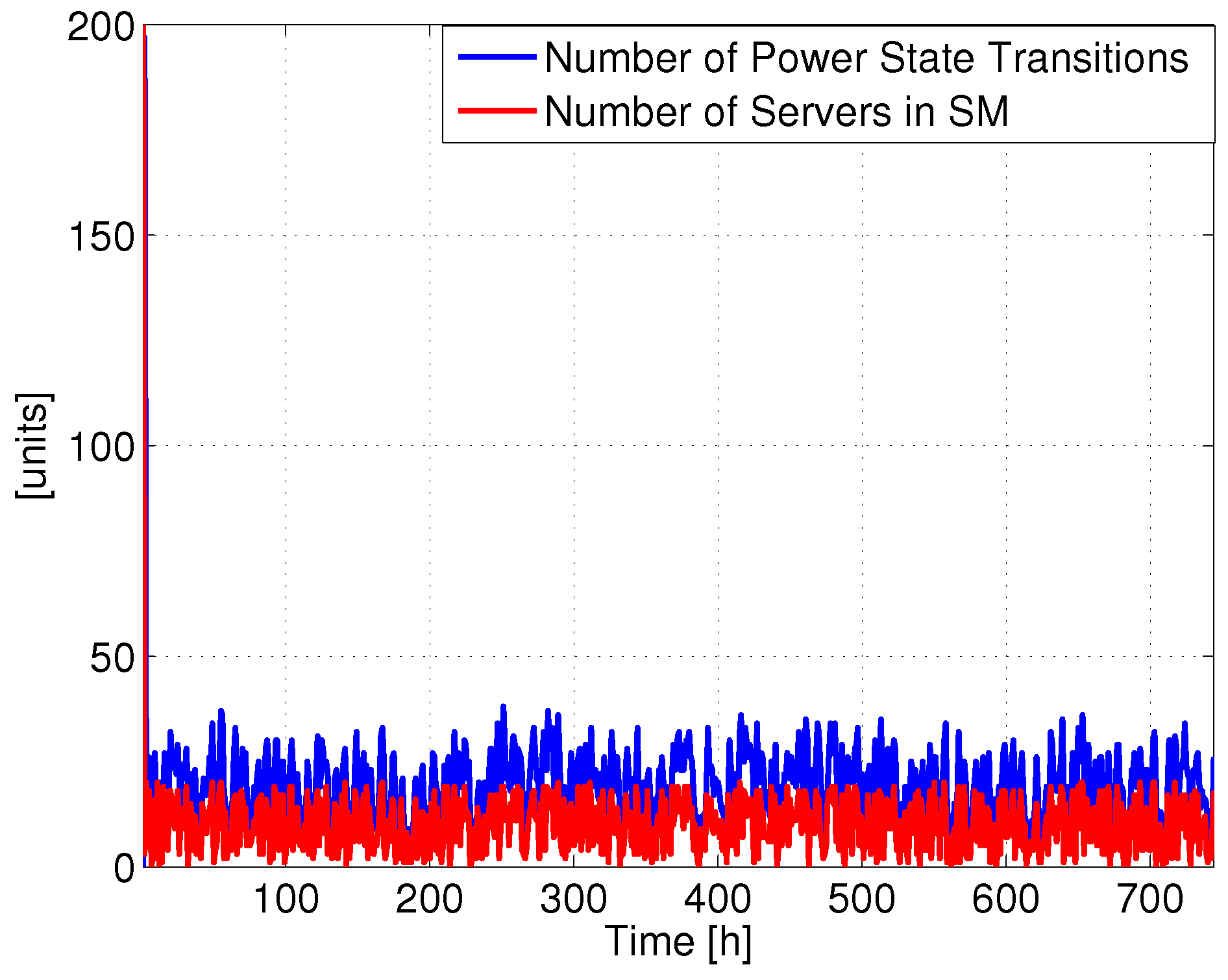
Figure 8 reports the number of power state changes involving SM and the total number of servers in SM
versus time. In contrast to the previous case (reported in
Figure 2), the number of SM power states and the transitions are pretty low, most of the servers being always active during the considered time period. More in depth, if we consider the number of power state changes
versus server ID (reported in
Figure 9), we can see that more than 50% of servers experience less than or equal to 70 transitions during
T, corresponding to less than 2.2 transitions per day. Moreover, we can clearly see that no transitions between active states are experienced, suggesting that a transition always implies a passage between full power and SM (or
vice-
versa).
We then apply our model also in this case.
Figure 10 reports the variation of the HW parameters
and
. Interestingly, since most of the servers are always powered on, the resulting AF is close to one. However, also in this case we can see that as
increases, the AF tends to be higher than one at the end of the considered time period.
6.2. Energy Minimization Impact
In the last part of our work, we consider the impact of setting an energy-minimization strategy in the DC. When , the energy is minimized. However, the delay is unbounded and therefore all the servers are always put in SM in each time slot, independent of the amount of traffic requests. To overcome this issue, we set in order to reduce energy while also considering the delay.
Figure 11 reports the number of power state changes and the number of servers in SM
versus time. Interestingly, most servers are always put in SM, and they are activated in order to serve the traffic requests. Consequently, there are different transitions introduced. By considering the power state changes
versus the server ID (reported in
Figure 12), we can see that around 50% of servers do not experience any transitions. However, for the subset of servers changing power state, we can see that even transitions between active power states are experienced.
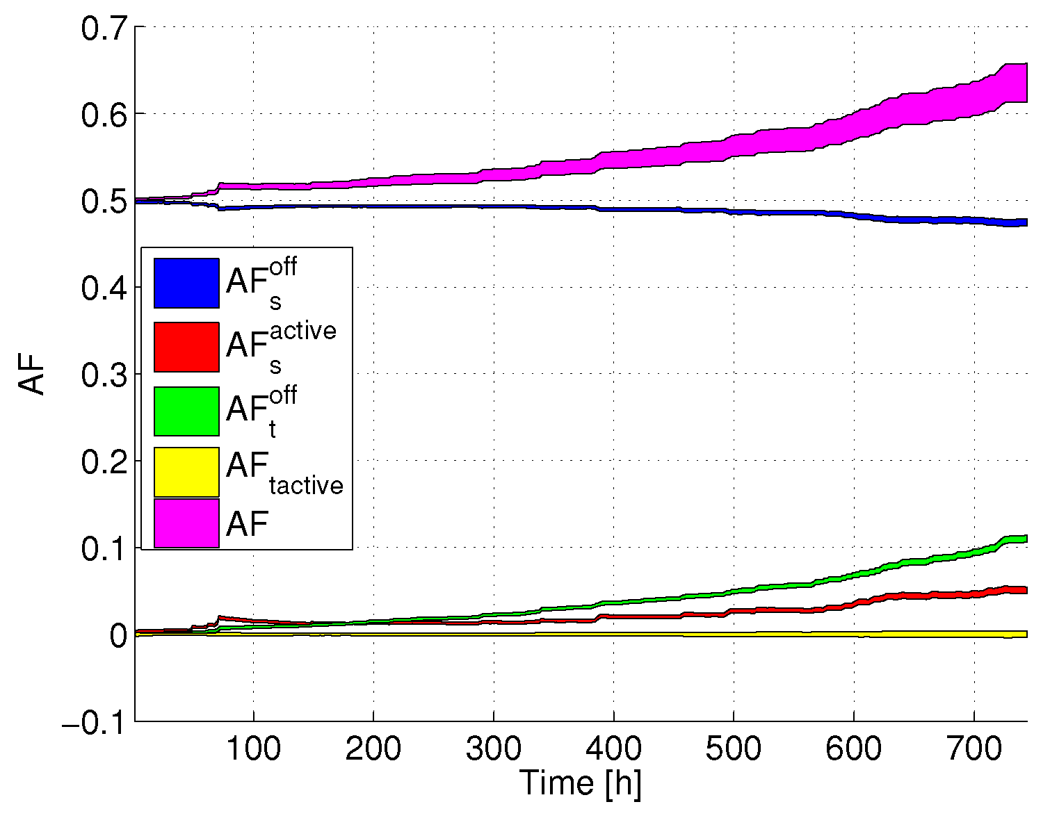
Figure 13 reports the AF
versus time in this scenario, considering a variation of the HW parameters
and
. Interestingly, in this case the AF is always lower than one, leading to a lifetime increase with respect to the reference case, in which the servers are kept at full power . In particular, although the AF tends to increase when
is increased (as expected), this effect is counterbalanced by the fact that many servers are always in SM, resulting in a low AF. In fact, if we consider the different AF components (reported in
Figure 14 for the case
,
(cycles/h), and
), we can clearly see that the largest contribution on the final AF is brought by
in this case, resulting in a lifetime increase.
6.3. Discussion
In the following, we will briefly discuss the main issues emerging from our work.
6.3.1. Impact of Scenario
In this work, we have evaluated a server lifetime model in cloud DCs. Clearly, the presented results depend on the specific scenario taken under consideration. In particular, we have considered the same number of servers deployed in each DC. However, if the number of deployed servers is not the same across the set of DCs, we may expect differences in the AF experienced by the servers in each DC. For example, when the number of deployed servers in a specific DC is above the average number of deployed servers per DC, we may expect that different servers may be put in SM, thus decreasing their AF. On the contrary, when the number of deployed servers is lower than the average, then almost all the servers will always be in active mode, thus increasing their AF. Moreover, the workload characteristics may impact the power usage, and consequently the results.
In addition, the considered time slot duration (i.e., 1 h) is sufficient to capture temperature variations triggered by power state variations. In general, temperature is more inertial than power state change and it is accumulated from continuous work state, regardless of power increase or decrease. In other words, temperature variation is less than power state change. For example, although processor frequency is decreasing, the processor temperature will increase after working for a while. In our case, this phenomenon may appear when very short time slot durations are taken into account (i.e., in the order of seconds or a minute). As a consequence, the presented model may not be valid in these cases, since the temperature will not change with power. We leave the investigation of models tailored to shorter time slot changes as future work.
6.3.2. Impact of Hardware Components Failures
A server is composed of different HW components—such as processors, disks, memory, etc.—which may have different failure patterns. Our work aims at the definition of a lifetime model for the whole server (and not for each component). In particular, when a server fails, there is a QoS degradation for users (almost independent of the specific component that fails). As a consequence, we are interested in the lifetime expressed as the mean time of the two failure events, independent of the components that have triggered the failures. We leave the investigation of more specific models tailored to specific components as a future work.
6.3.3. Other Factors Influencing Failures
Except for the normal worn-out parts, server failures may be triggered by different factors, including: overheating, defects in the chip, operation outside the design specifications, power surge/fluctuation, over-voltage, and overheating. For example, focusing on hard disks, temperature, impact, exposure to water or high magnetic fields, or dust environment may also contribute to its failures. Our model instead takes into account only the failures triggered by power state changes. Nevertheless, all these other failures (which do not depend on the power state changes) can be taken into account in the reference failure rate—i.e., the failure rate achieved by keeping a constant power, introduced in the definition of the AF metric. Our model then reports the variation of lifetime with respect to the reference failure rate.
6.3.4. Data Center Thermo-Mechanical Physical Design
The study of the materials’ properties as they change with temperature is the scope of the thermo-mechanical analysis. A branch of this analysis is devoted to the DC physical design. In this context, this work falls within the scope of modulated temperature conditions with static force applied. Actually, we assume that no force is applied on the material, and the resulting AF is solely the result of power (and hence temperature) variations. In general, predicting the lifetime of electronic components is not a trivial task, and different works in the literature detail experimental data of electronic components’ lifetime. For example, the authors of [
20] focus on solder joint interconnections, which are considered to be the weaknesses of microelectronic packaging. In particular, the authors conducted an accelerated temperature cycling in a thermal chamber, where temperatures range between a minimum and a maximum value. Then, after the thermal cycling was completed for different numbers of cycles, two samples were extracted, prepared, and then analyzed with a scanning electron microscope to characterize the microstructures and to collect failure data. The authors clearly show that the failure probability (called unreliability) increases with the number of cycles. Focusing then on the AF models, the authors of [
21] provide a comprehensive overview for joint solders. In our case, we are characterized by relatively short dwell times (
i.e., the time between reaching a given power state from another one) and pretty large variations of power (especially when passing from/to SM). Therefore, plastic strain-based fatigue models [
21] (like the Coffin–Manson one) can be exploited. We recognize, however, that creep strain-based fatigue models [
21] may be assumed when considering transitions between active power states (especially when occurring between the highest power states). Actually, one of possible future research activities will be to measure the AF for a set of server machines and then to follow the methodology proposed by [
21] for selecting the applicable fatigue models (and their parameters).
Finally, it is worth mentioning that an optimized lifetime-aware management of DCs could also have implications on the provisioning of air conditioning [
22], as well as reducing active redundant air conditioning systems.


