An Adaptive Energy Management System for Electric Vehicles Based on Driving Cycle Identification and Wavelet Transform

Abstract

Since driving cycle greatly affects load power demand, driving cycle identification (DCI) is proposed to predict power demand that can be expected to prepare for the power distribution between battery and supercapacitor. The DCI is developed based on a learning vector quantization (LVQ) neural network method, which is assessed in both training and validation based on the statistical data obtained from six standard driving cycles. In order to ensure network accuracy, characteristic parameter and slide time window, which are two important factors ensuring the network accuracy for onboard hybrid energy storage system (HESS) applications in electric vehicles, are discussed and designed. Based on the identification results, Multi-level Haar wavelet transform (Haar-WT) is proposed for allocating the high frequency components of power demand into the supercapacitor which could damage battery lifetime and the corresponding low frequency components into the battery system. The proposed energy management system can better increase system efficiency and battery lifetime compared with the conventional sole frequency control. The advantages are demonstrated based on a randomly generated driving cycle from the standard driving cycle library via simulation.

1. Introduction

Electric vehicles are considered as one of the most promising transportation tools for addressing issues faced by automotive industry worldwide on energy and environment [1,2,3,4]. Technologies employed for all kinds of electric vehicles are various, but their performances are largely dependent on the characteristics of adopted energy storage system (ESS) [5,6]. Of all the ESSs, batteries are one of the most widely used energy sources for electric vehicles, which has been an emerging area for ensuring a successful application of electric vehicles. However, batteries alone as a power source have faced some challenges for practical engineering applications, such as higher energy efficiency, smaller voltage drops, larger vehicle acceleration or deceleration rates, better uphill climbing performance. Although high-power batteries can be made available, they are very bulky and cost prohibitive [7,8].

To solve the dilemma, a supercapacitor can be added onboard to form a hybrid energy storage system (HESS) such that the battery and the supercapacitor each play a complementary role based on their individual dynamic characteristics [9,10]. The battery has high energy density, relatively low cost per watt-hour, but low specific power, and short lifetime; while the supercapacitor possesses higher power density, longer cycle life, but relatively lower energy density and higher cost per watt-hour [11,12,13,14]. Consequently, a combination of these two types of ESSs will yield an equivalent ESS with both higher energy density and higher power density, where energy is stored in the battery and power is supplied by the supercapacitor. In this way, sudden peak currents in the battery, which would result in a large reduction in lifetime [15,16], can be avoided effectively. Besides, electric vehicle range can also be extended because of the high utilization of the regenerative breaking [17].

In order to encourage the development of the HESS, mounting research efforts have been devoted to improving the system performance from both low level topology structure [18,19,20,21] and high level energy management [22,23,24,25,26,27,28,29,30,31,32,33,34,35,36]. In the literature, a number of hybridization topology structures where the supercapacitors have been implemented in combination with battery systems. These structures can be mainly categorized into passive, semi-active and fully active types according to the control pattern of each power source. In the passive structure, none of the bidirectional direct current (DC) converter is used for power distribution between the battery and supercapacitor. The distribution is inherently achieved by the internal resistances of power sources thus the energy stored in the supercapacitor cannot be utilized effectively. In the semi-active structure, only a single bidirectional DC converter is used to control the operation of just one of the power sources. Therefore, only one freedom can be found in this structure. In order to maximize the system freedom, the fully active structure adopts two bidirectional DC converters such that the hybrid system can be decoupled fully. By comparing the three structures, it can be found that the passive hybrid system is simple in structure and more cost effective, but the fully active hybrid system offers the best performance. Therefore, a semi-active hybrid system is often a good trade off among them in terms of the performance, the structure complexity and the cost.

Based on these topology structures, various energy management control strategies for a battery and supercapacitor HESS are also developed in the literature. These strategies can be broadly classified into rule-based and optimization-based distribution. Rule-based controllers are referred as deterministic rule, learning network and fuzzy logical controller. In [22], an advanced vehicle simulator (ADVISOR)-based battery and supercapacitor HESS was developed, the power distribution rule between battery and supercapacitor was determined based on an experiment approach. In [23], an integrated rule-based meta-heuristic approach was presented, and simulation results have proved the effectiveness of this multi-level energy management system (EMS) fulfilling the requested performance with better source usage and much lower installed capacities. In [24], a fuzzy logical controller based on particle swarm optimization algorithm was presented to achieve optimization power flow distribution between battery and supercapacitor. Reference [25] adopted the idea of neural networks and developed an efficient energy management system for hybrid electric vehicles with closed form approaches (more can be found in [26,27,28,29]).

Optimization-based methods consider local and global optimization problems by using past driving cycle information to determine the power distribution mode among power sources. Reference [30] formulated an optimization problem by considering the minimization of the magnitude/fluctuation of the current flowing in and out of the battery and the energy loss of the supercapacitor. A model predictive control (MPC) controller for a hybrid battery-supercapacitor power source was proposed and experimentally verified in [31]. The designed MPC controller enables the battery to share the low frequency power components and the high frequency power components are allocated to the supercapacitor. In [34], a wavelet transform-based power management strategy was proposed, in which load power is decomposed into different frequency components to the fuel cell (FC), battery and supercapacitor, compatible with their respective dynamic characteristics. Reference [35] adopted a first-order low-pass filter, which was designed for frequency decomposition along with analysis of components responses under real world driving cycles. These strategies would increase battery lifetime attributing to effective frequency separation consideration. Recent research related to multimode energy management based driving cycle prediction and multi-criteria integrated optimization problem are proposed in [36,37].

From prior research described in the literature, a large proportion of work has focused on the power distribution method development among power sources based on a certain driving cycle. However, the problem that strategies verification based on a certain composite test cycle comprising of various driving cycles information is not yet discussed. In this paper, a driving cycle identification (DCI) based frequency separation energy management system for electric vehicles is proposed to deal with power distribution between battery and supercapacitor. The proposed energy management system is a two-level structure. In the first level, a DCI system based on a learning vector quantization (LVQ) neural network method is developed, whose role is to identify the type of driving cycles based on a series of statistical characteristic parameters. The identification results are subsequently used by the second level, in which multi-level Haar wavelet transform (Haar-WT) is employed for allocating load power into the high-low frequency components. In order to gain high identification accuracy, eighteen characteristic parameters, which are extracted from six standard driving cycles, are described and analyzed. Simulation results have shown that the proposed eighteen characteristic parameters are able to ensure high identification accuracy compared with other characteristic parameters. Furthermore, a slide time window is proposed and designed to dynamically extract characteristic parameters thus reducing sampling time consumption while improving calculation efficiency. Finally, the energy management system is validated under the MATLAB/Simulink environment and then tested based on a randomly generated driving cycle from the standard driving cycle library. Simulation results have shown that the energy management system is able to adjust the high-low frequency power components effectively to adapt the variations of driving cycles. Compared with conventional sole frequency controls, the proposed energy management system can well balance the voltage of supercapacitor by adjusting the combination of separation frequency and thus can ensure effective peak power supply by supercapacitor without over-discharging supercapacitor.

The rest of this paper is organized as follows: Section 2 develops the models of the HESS. Section 3 describes method for the proposed energy management system. The real-time simulation is carried out to evaluate the performance of energy management system in Section 4. Finally, the paper is concluded in Section 5.

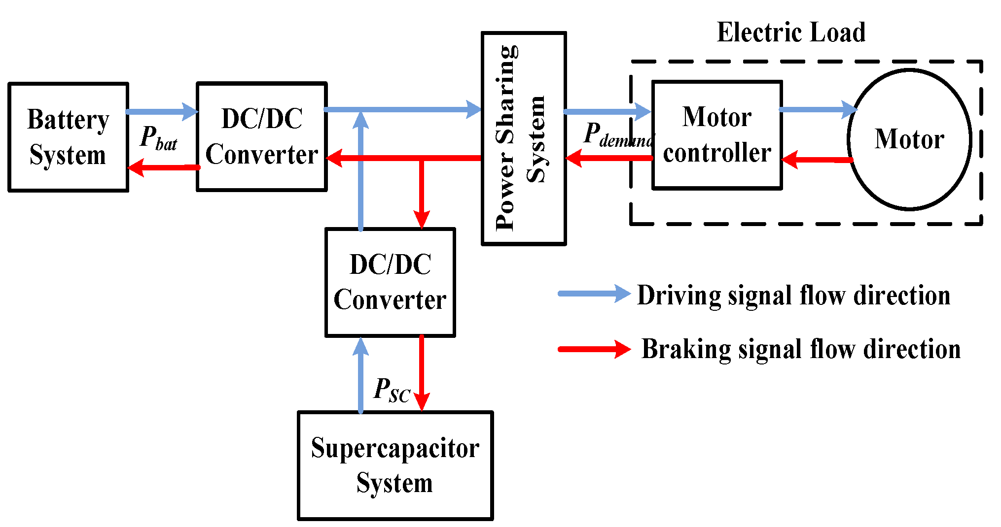
2. Model Development of the HESS

The considered system configuration is shown in Figure 1. The described topology is a full-active structure with a double-conversion system. The battery system consists of 74 cells in series, and each cell has a 3.8 V nominal voltage. The supercapacitor system consists of 55 cells in series, and each cell has a 2.7 V nominal voltage. The electric vehicle is powered by a 30 kW permanent magnet synchronous motor (PMSM) with a maximum torque of 150 Nm.

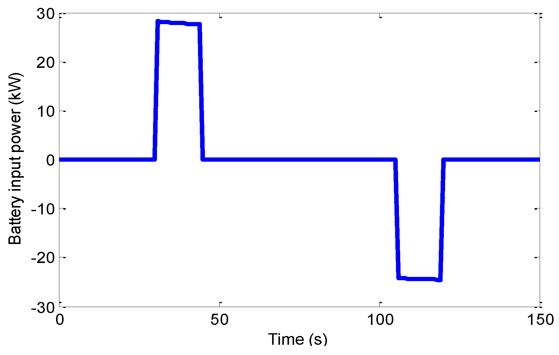
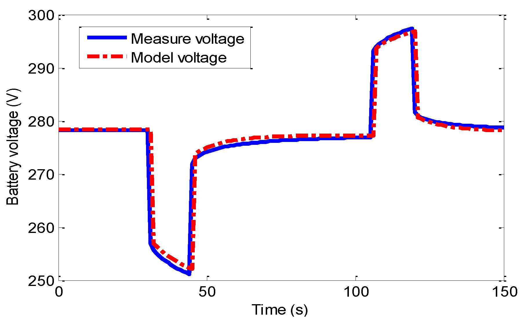
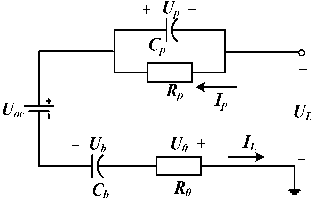
2.1. Dynamic Model of the Battery

Lithium-ion batteries have higher energy density than any other types of batteries, roughly twice as much energy density as nickel metal hyoride (NiMH) batteries do. Therefore they are an ideal candidate for electric vehicle applications. In the research, a ternary lithium-ion battery is considered as the main energy storage unit capable of coping with the base load and the low-dynamic variations of load power.

Compared with other battery models, the Partnership for a New Generation of Vehicles (PNGVs) model has more high voltage accuracy and is thus more suitable for modeling lithium-ion battery [38]. Its equivalent electric circuit is shown in Figure 2. The model consists of one resistance and capacitor (RC) pair that describes the double layer effect, which is a fast dynamic process with a time constant ranging from hundreds of milliseconds to several seconds. $U_{oc}$ represents an ideal voltage source, and is used to describe the battery open-voltage; $R_0$ is ohm resistance; $C_b$ is used to describe the open-voltage fluctuation resulting from the time accumulation of load current; Polarization resistance $R_p$ and polarization capacitance $C_p$ are used to describe the battery’s over-voltage $U_p$, which is used to describe the dynamic characteristics of the battery; $I_L$ and $U_{L }$are the current and voltage of the battery, respectively.

State of Charge (SoC) is traditional used to indicate the residual electricity of battery, its definition is usually written by [2]:

$$\mathrm{SoC}={\mathrm{SoC}}_0-k_{ch}·k_{dis}·{{\displaystyle \int }}^{\text{}}\epsilon ·I_{bat}\mathrm{dt}/C_{bat}$$

(1)

where ${\mathrm{SoC}}_0$ describes the initial value of SoC; $k_{ch }\mathrm{and} k_{dis}$ describes the impact coefficients on the current integration from charging current ($I_L<0$) and discharging current ($I_L>0$) respectively. If the battery is charging, $k_{dis}=1$, if the battery is discharging, $k_{ch }=1. C_{bat}$ describes the nominal capacity of battery, $\epsilon$ is the coulomb efficiency (including charging efficiency ${\epsilon }_{ch}$ and charging efficiency ${\epsilon }_{dis}$). The main state equations for the PNGVs battery model are written by Equations (2)–(4) [38]:

$$\left[\begin{array}{c}{\dot{U}}_b\\ {\dot{U}}_p\end{array}\right]=\left[\begin{array}{c}0 0 \\ 0 -1/\left(C_p{R}_p\right)\end{array}\right]·\left[\begin{array}{c}{U}_b\\ U_p\end{array}\right]+\left[\begin{array}{c}1/C_b\\ 1/C_p\end{array}\right]·I_L$$

(2)

$$U_L=\left[-1 -1\right]·\left[\begin{array}{c}{U}_b\\ U_p\end{array}\right]-R_0·I_L+U_{oc}$$

(3)

$$I_L=\left\{U_{oc}-U_b-U_p-{\left[{\left(U_{oc}-U_b-U_p\right)}^{\frac{1}{2}}-4·R_0·P_L\right]}^{\frac{1}{2}}\right\}/\left(2·R_0\right)$$

(4)

where the terminal voltage of capacitor $C_b$ can be calculated by the load current integration, as is described in Equation (5):

$$U_b={{\displaystyle \int }}^{\text{}}{I}_L·\mathrm{d}t$$

(5)

The polarization voltage and current can be written as follows:

$$U_p=R_p·I_p$$

(6)

$$I_{p,k}=\left(1-\left\{1-\exp \left(-T\right)\right\}/T\right)·I_{L,k}+\left(\left\{1-\exp \left(-T\right)\right\}/T-\exp \left(-T\right)\right)·I_{L,k-1}+\exp (-T)·I_{p,k-1}$$

(7)

where $T=\Delta t/\tau$, and $\Delta t$ represents sample time, $\tau$ represents battery time constant. Then the available load power can be calculated using the multiplication of current and voltage as follows.

$$P_L=U_L·I_L$$

(8)

Finally, the model of PNGVs battery can be developed under the Simulink environment of MATLAB using the relations described in Equations (1)–(8).

A charging/discharging experiment of a maximum voltage 300 V lithium-ion battery pack is carried out to validate the developed battery model. The charging/discharging power is shown in Figure 3. Figure 4 illustrates the experimental results compared to the simulation carried out using MATLAB/Simulink for the charging/discharging test at the same input power, which describes a good correlation between each other.

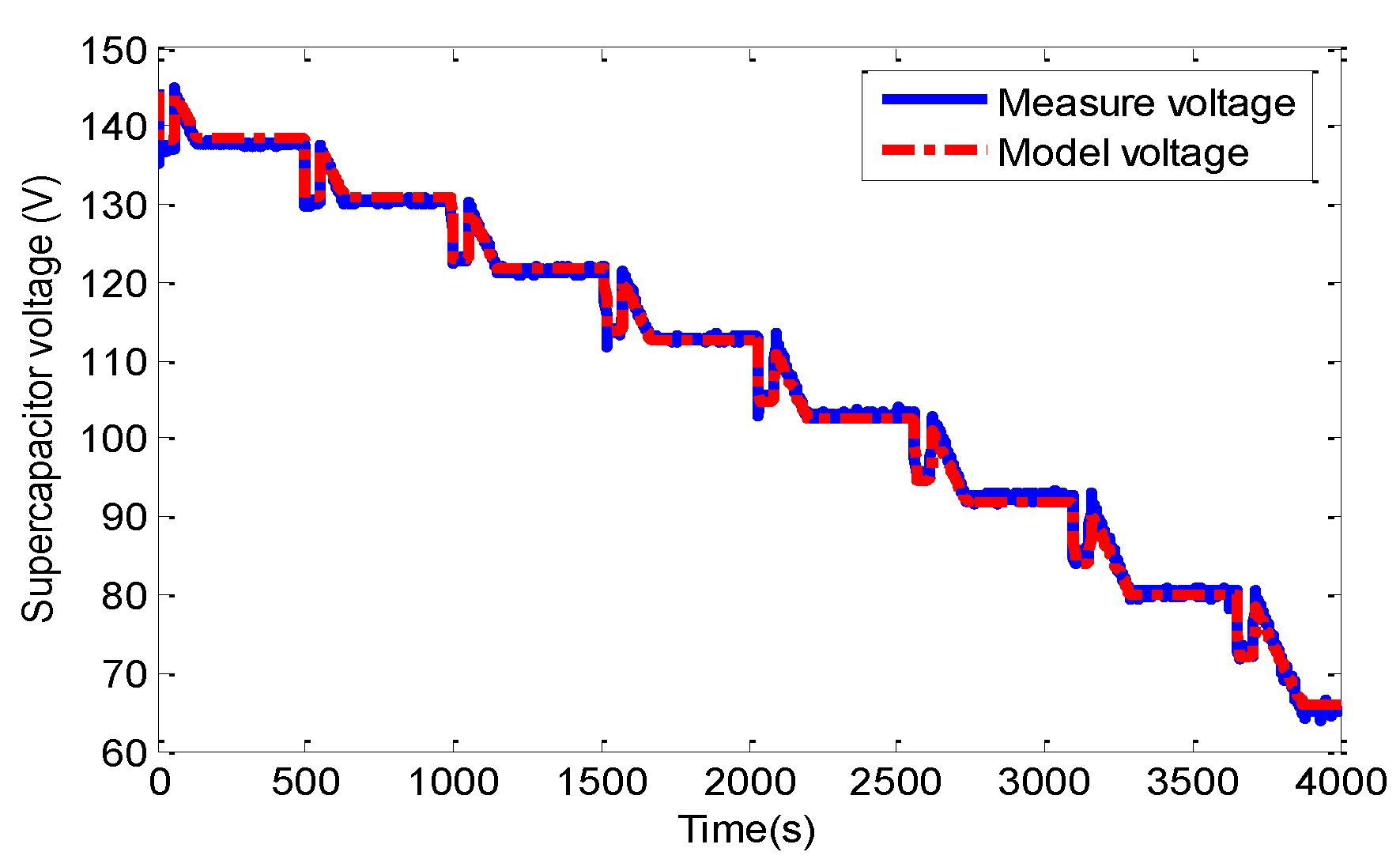
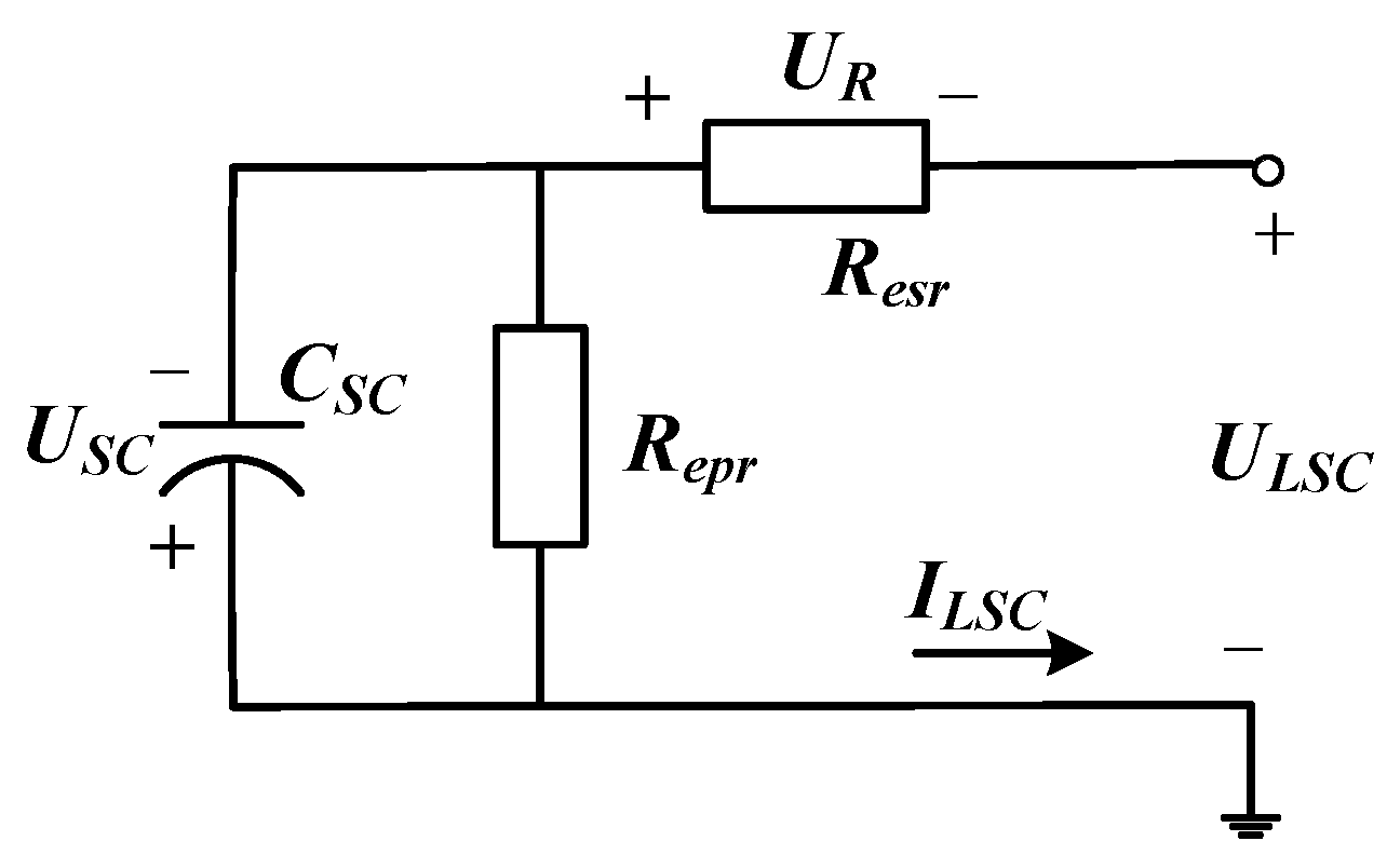
2.2. Dynamic Model of the Supercapacitor

Supercapacitors have a wider working range, higher working efficiency and longer cycle life than that of batteries. On the other hand, as the power-assisted ESS, it has the characteristics of high-power density and relatively low internal resistance compared with a battery, so it is available for providing high power bursts to meet the power demand of electric vehicles. In this subsection, the mathematical modeling of the supercapacitor system used in the research is presented. Figure 5 shows the RC equivalent circuit of the supercapacitor. The model consists of a capacitance C and an equivalent parallel resistance $R_{epr}$ representing the self-discharging loss, an equivalent series resistance $R_{esr}$ representing the charging/discharging resistance. The $R_{epr}$ models the leakage affects and only impacts the long term energy storage performance of the supercapacitor [39].

From Figure 5, the load voltage of supercapacitor can be written by Equations (9) and (10) respectively:

$${\dot{U}}_{SC}=-U_{SC}/\left(C_{SC}·R_{epr}\right)+I_{LSC}/C_{SC}$$

(9)

$$U_{LSC}=U_{SC}-R_{esr}·I_{LSC}$$

(10)

In order to indicate the residual electricity of supercapacitor, The State of Voltage (SoV) is used to describe as a percentage of the rated energy capacity, which depends on the terminal output voltage and is defined as [2]:

$$\mathrm{SoV}=\left(U_{LSC}-U_{cmin}\right)/\left(U_{cmax}-U_{cmin}\right)$$

(11)

where $U_{max}$ and $U_{min}$ are the maximum and minimum terminal voltage respectively.

A charging/discharging experiment of maximum voltage 150 V Maxwell supercapacitor pack is carried out to validate the developed model and the charging/discharging power is shown in Figure 6. Figure 7 illustrates the experimental results compared to the simulation carried out using MATLAB/Simulink for the charging/discharging test at given input power. It can be observed that the supercapacitor model is in very good agreement with the experimental result.

2.3. DC/DC Converter and Motor Models

The bidirectional DC/DC converters are usually used for the battery and supercapacitor system to stabilize their voltage variations. In this research, the DC/DC converter models are assumed to be the energy efficiency evolving in function of the output power, which are described in Equations (12) and (13) respectively:

$$P_{bat}=1/{\eta }_{dc}\left(P_{dc}\right)·P_{bat,DC}$$

(12)

$$P_{SC}=1/{\eta }_{\mathrm{dc}}\left(P_{\mathrm{dc}}\right)·P_{SC,DC}$$

(13)

where ${\eta }_{dc}$ represents DC converter efficiency, $P_{bat,DC}$ represents input power of the DC converter connecting the battery, $P_{SC,DC}$ represents input power of the DC converter connecting the supercapacitor. In order to describe the impact of electric motor dynamics on load power demand of the HESS, the electric motor is modeled as a first-order delay link, which is described in Equation (14):

$$P_{motor, out}=P_{motor,in}·\exp (-t/{\tau }_m)$$

(14)

where $P_{motor,in}$ represents the input power of the electric motor, $P_{motor, out}$ represents the output power of the electric motor, ${\tau }_m$ represents the time constant of the electric motor. For the sake of simplicity, the time constant is considered as a constant.

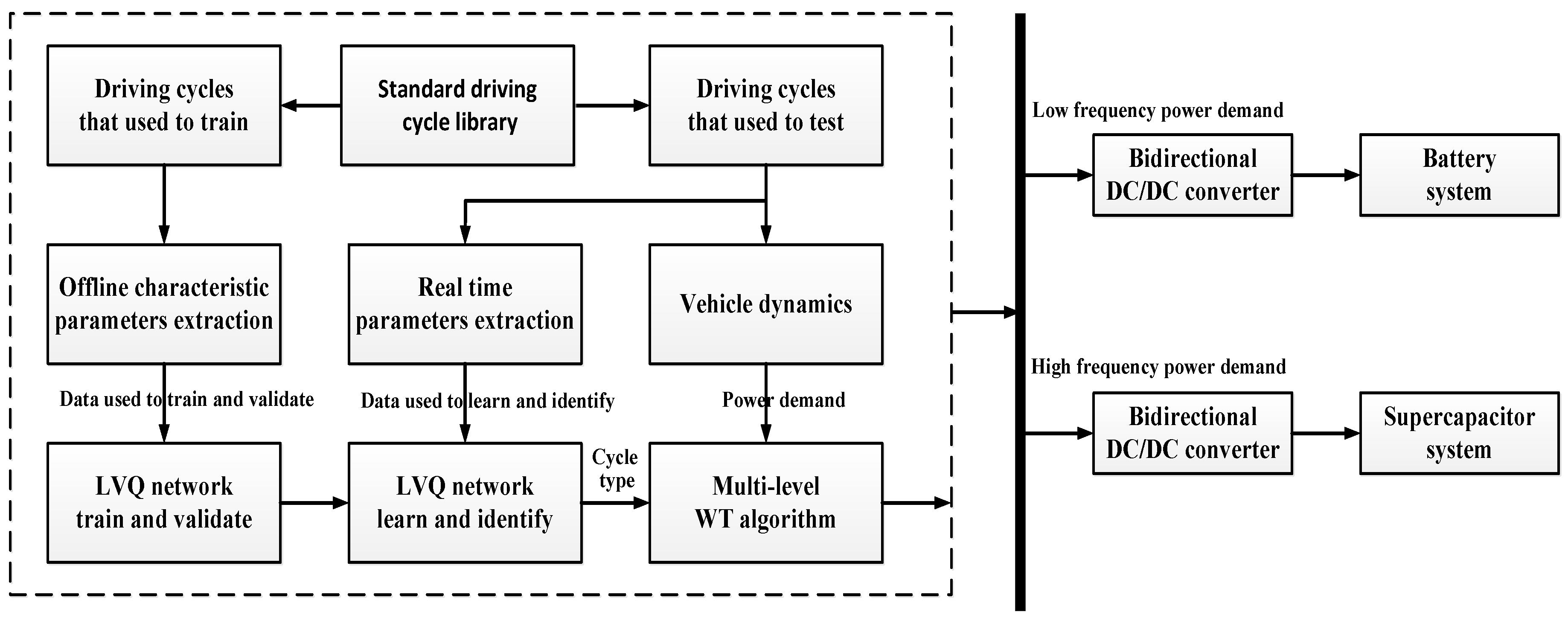
3. Energy Management System Based on DCI and Haar-WT

3.1. DCI Method

The LVQ neural network method has been widely used in the control field for prediction and identification because of its effectiveness and high accuracy [40,41,42], and thus it is proposed to identify the types of driving cycles in this work.

The structure of the LVQ neural network is shown in Figure 8, which comprises an input layer, competitive layer and linear layer. The input layer is fully connected to the competitive layer by neurons, but the competitive layer is connected to the linear layer by neurons partly. As shown in Figure 8, the input vector X = [X₁, X₂,…, X₁₈] represents 18 characteristic parameters extracted from six standard driving cycles. I represent the input layer; W_i represents connection weight between input layer and competitive layer. The neurons H in the competitive layer C compute the Euclidean distance between the given input vector P and the prototypical vector W_i, namely ‖W_i − P‖, index represents the number of neuron. O represents the linear output layer.

In order to train the LVQ network for driving cycle identification, six standard driving cycles are selected as the train samples, which are shown in Figure 9. The six driving cycles are first categorized into three groups according to the amplitude and frequency of velocity. The INDIA_HWY_SAMPLE (Indian Highway Sample) and the HWFET (Highway Fuel Economy Test) driving cycles have highest velocity amplitude but lowest velocity frequency variations, which are considered as the highway cycle; the UDDS (Urban Dynamometer Driving Schedule) and the WVUSUB (West Virginia Suburban Driving Schedule) driving cycles have moderate velocity amplitude and moderate velocity frequency variations, which are considered as the moderate urban cycle; the INDIA_URBAN_SAMPLE (Indian Urban Sample) and the UKBUS6 (London Bus Route) driving cycles have lowest velocity amplitude but highest velocity frequency variations, which are considered as the congested urban cycle.

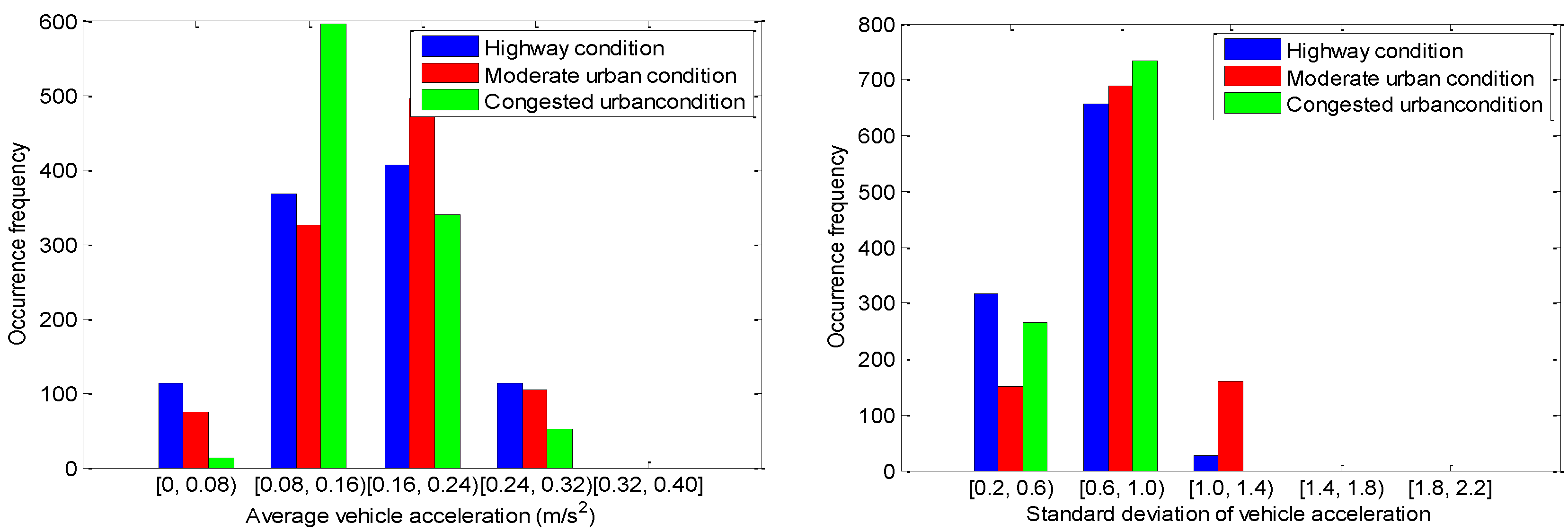
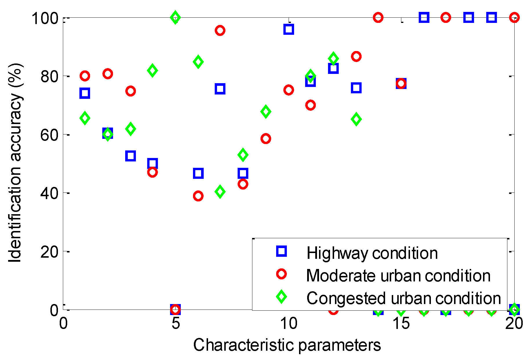
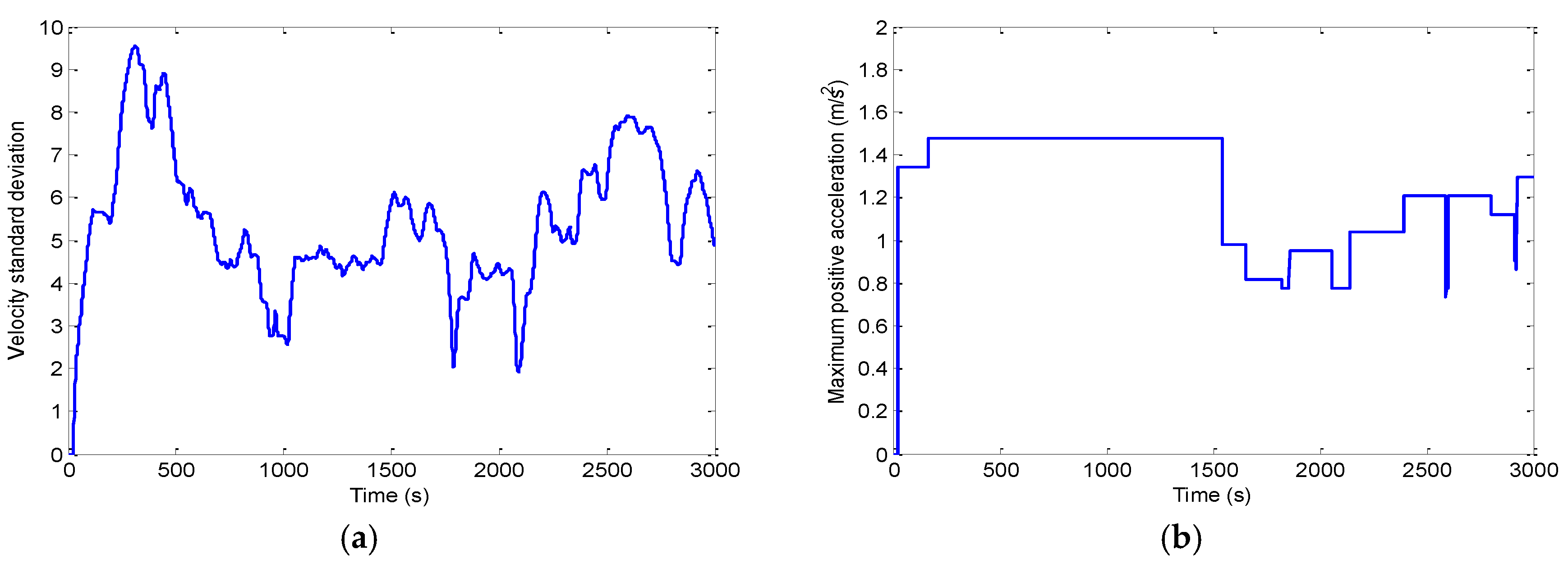
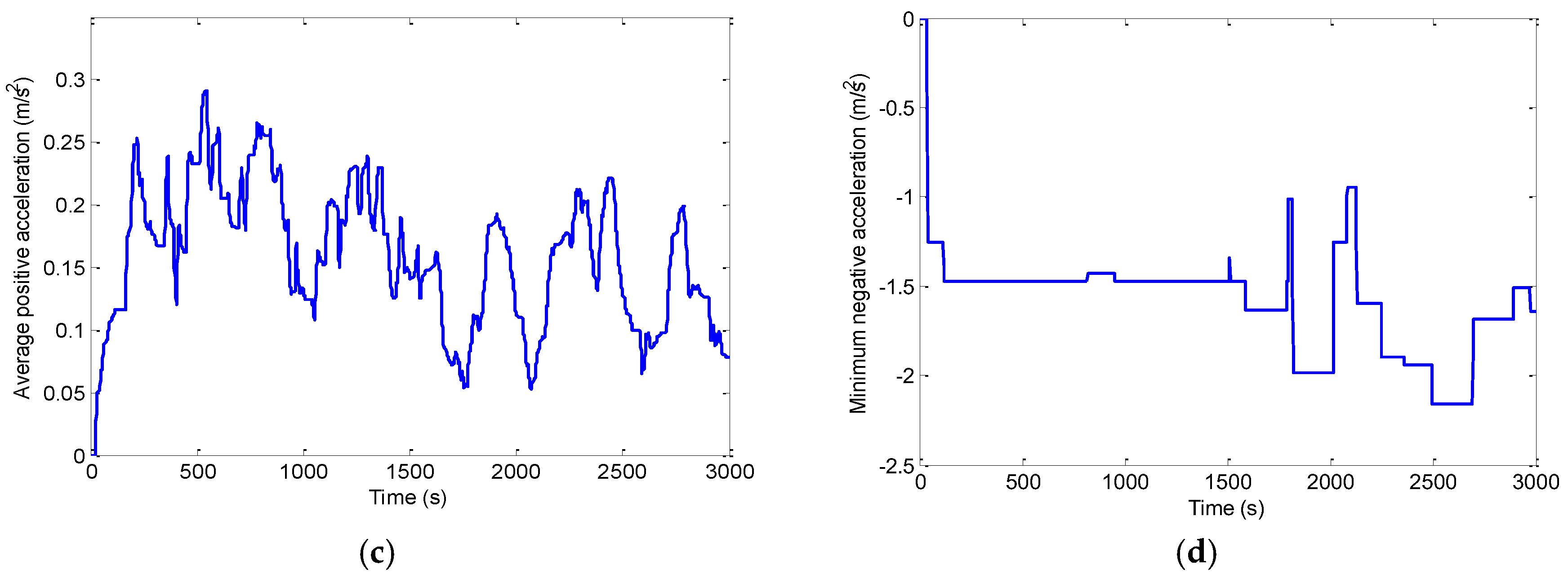
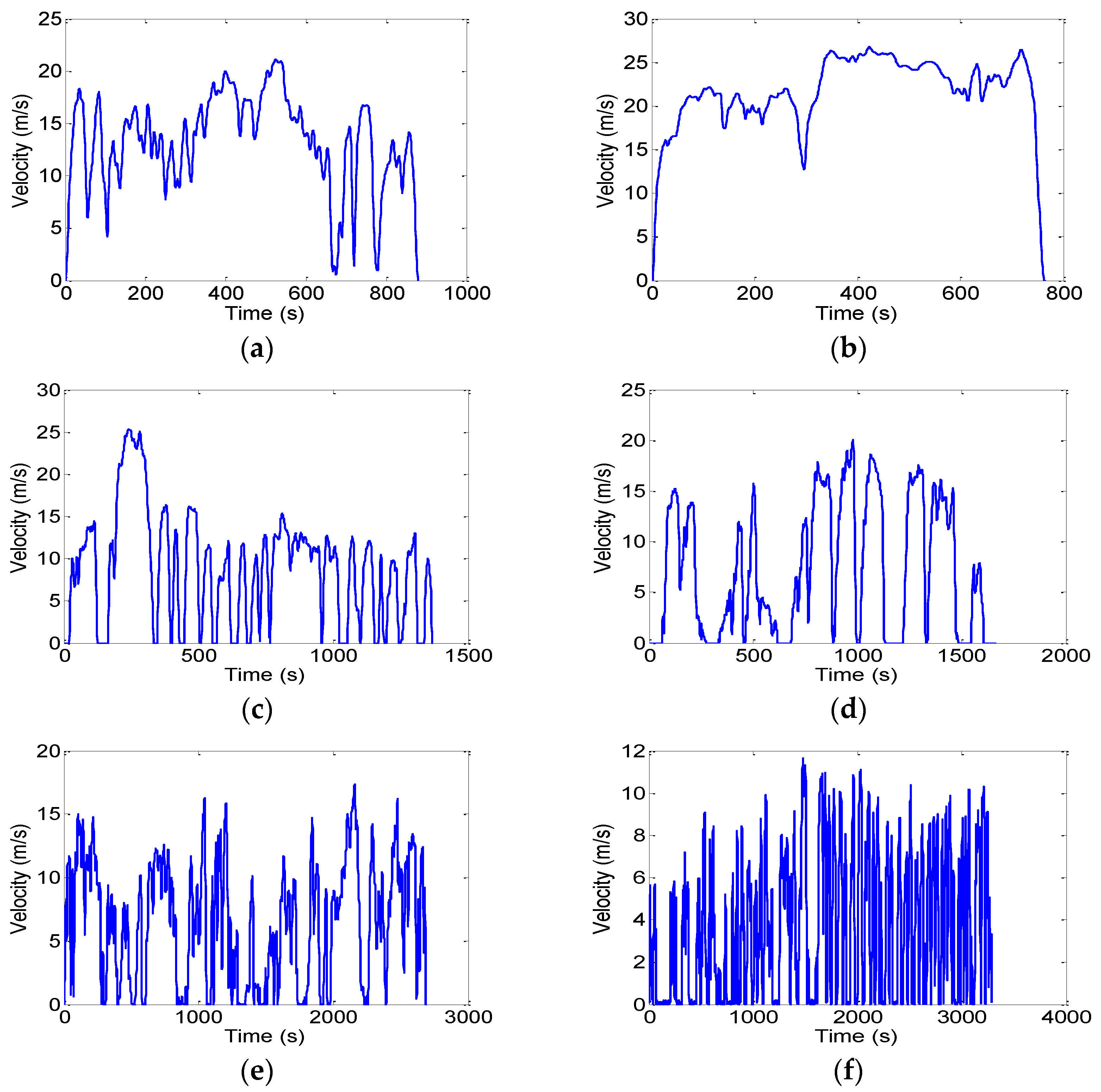
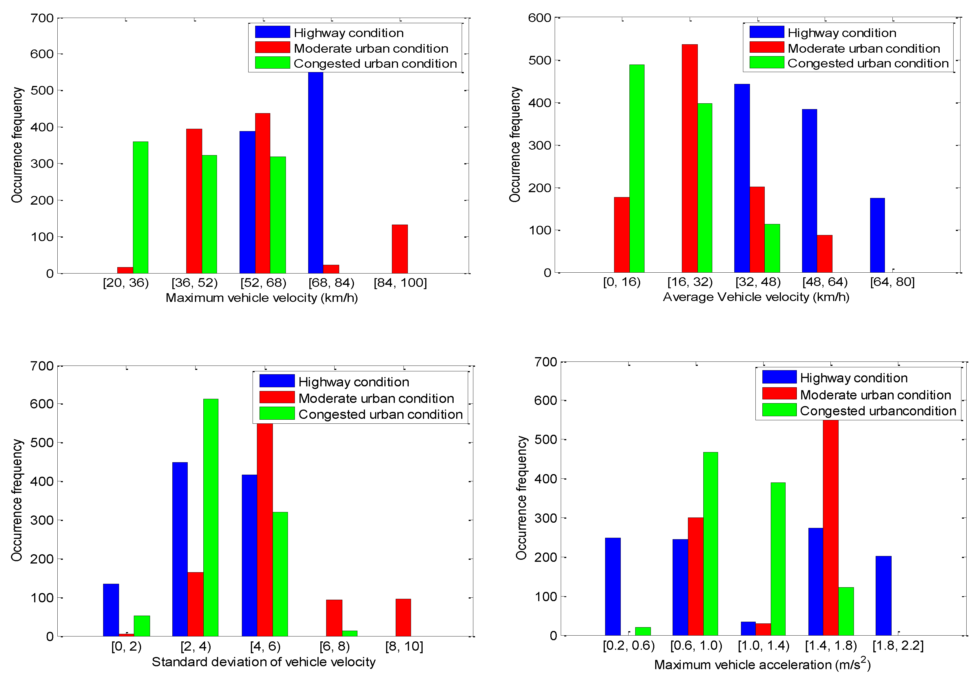
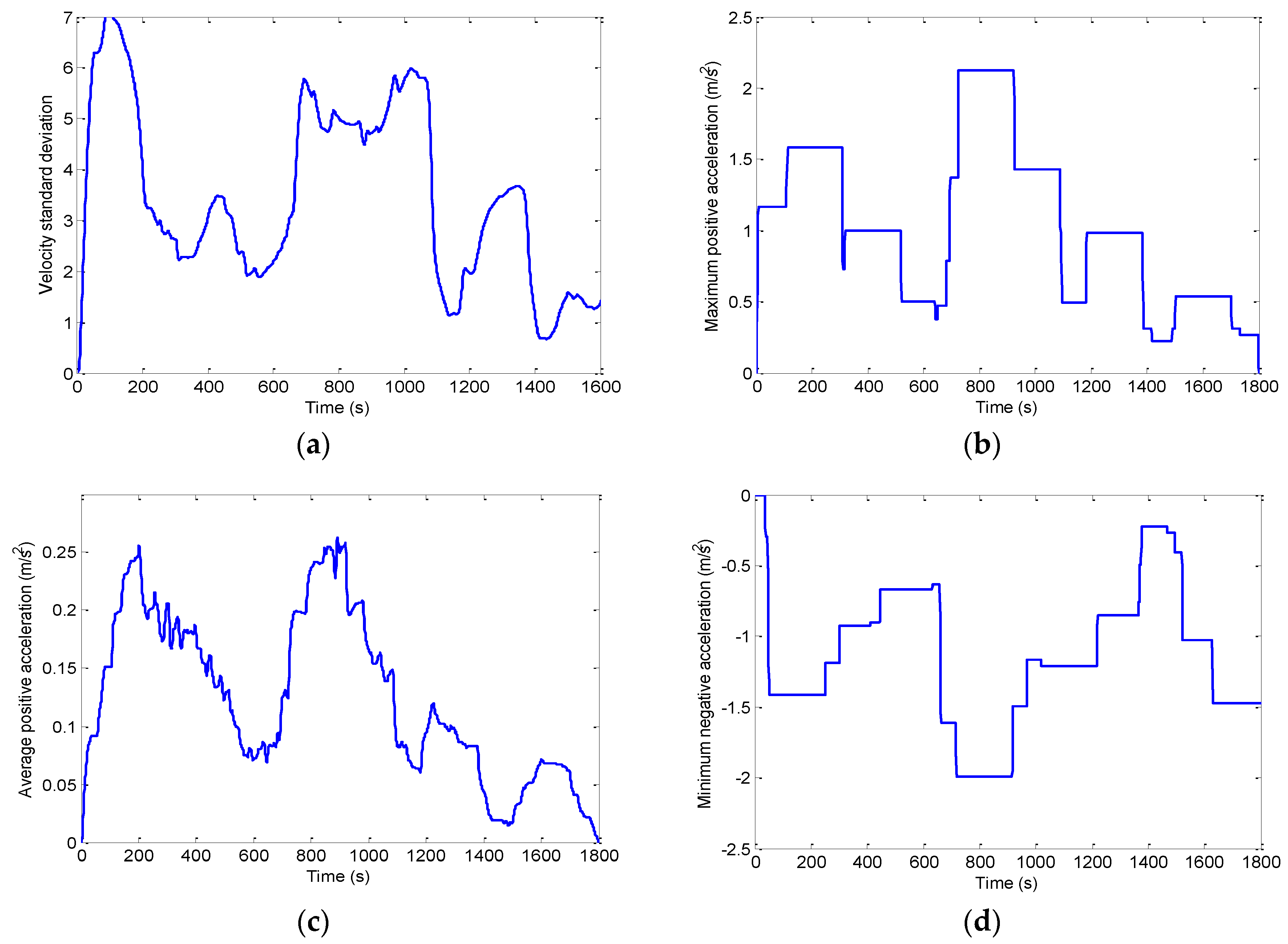
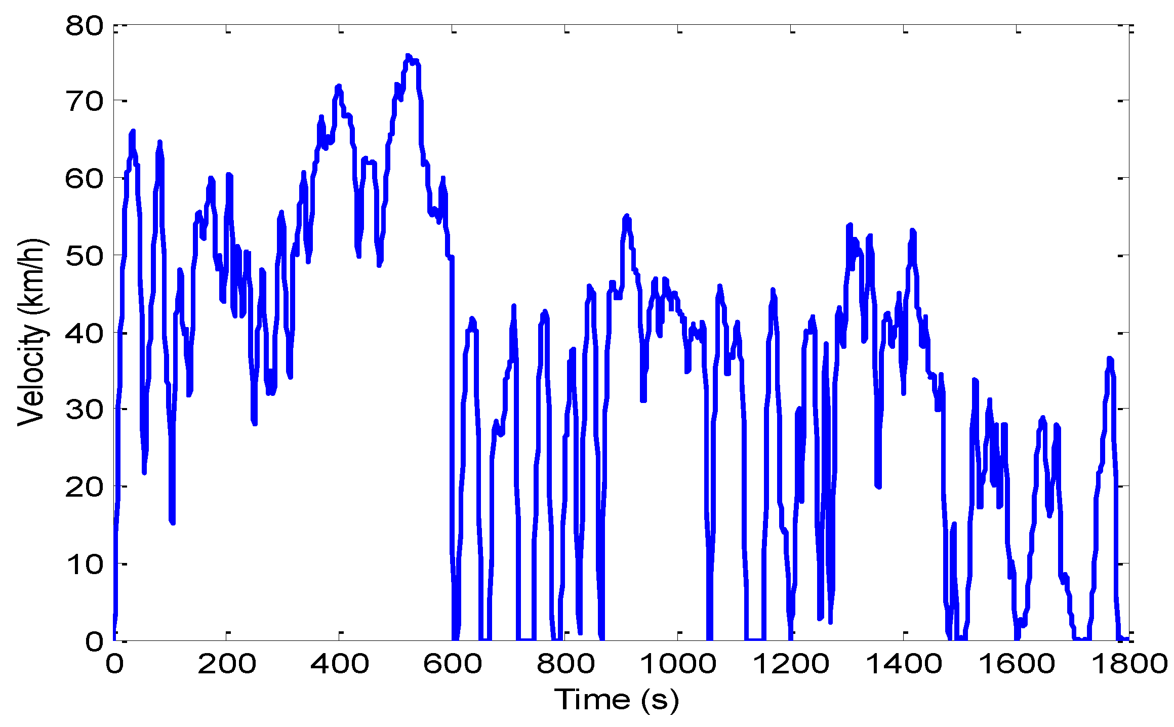
3.1.1. Characteristic Parameters Analysis

In order to obtain enough samples for characteristic parameter analysis, each group of driving cycles is divided into 1500 sample cycles, among which 1000 sample cycles are used to train the LVQ network, and 500 sample cycles are used to analyze characteristic parameters. The specific characteristic parameters are listed in

Table 1. Characteristic parameters of driving cycles.

Names and math description
Max velocity max(v(t))
Average velocity mean(v(t))
Velocity standard deviation std(v(t))
Max positive acceleration max(abs(a(t)))
Average positive acceleration mean(abs(a(t)))
Positive acceleration standard deviation std(abs(a(t)))
Max negative acceleration max(−abs(a(t)))
Average negative acceleration mean(−abs(a(t)))
Negative acceleration standard deviation std(−abs(a(t)))
Idle percent sum(v(t) = 0)/n
Constant velocity percent sum(a(t) = 0)/n
Velocity range percent 1 sum(v1 < v(t) < v2)/n
Velocity range percent 2 sum(v2 < v(t) < v3)/n
Velocity range percent 3 sum(v3 < v(t) < v4)/n
Positive acceleration range percent 1 sum(a1 < abs(a(t)) < a2)/n
Positive acceleration range percent 2 sum(a2 < abs(a(t)) < a3)/n
Positive acceleration range percent 3 sum(a3 < abs(a(t)) < a4)/n
Negative acceleration range percent 1 sum(a1 < −abs(a(t)) < a2)/n
Negative acceleration range percent 2 sum(a2 < −abs(a(t)) < a3)/n
Negative acceleration range percent 3 sum(a3 < −abs(a(t)) < a4)/n

. The comparison histograms of part characteristic parameters in each group of driving cycles are shown in Figure 10.

From Figure 10 we can observe that none of the characteristic parameters can make an ideal distinction among the three groups of driving cycles. Therefore, with a sole characteristic parameter it is difficult to identify all the cycles effectively, which can be further described in Figure 11. From Figure 11, although a sole characteristic parameter can guarantee a certain cycle high identification accuracy, it fails to ensure the high identification accuracy for all the cycles. To gain high identification accuracy for each group of driving cycles, a series of cross-validation methods are hereby proposed to obtain the optimal characteristic parameter combination. Fifty random tests are carried out for each group of characteristic parameters. Each test sample cycle is generated based on uniform distribution, thus repeated test can be avoided effectively. By simulation and comparison, six groups of characteristic parameters are finally determined. The identification results and accuracy comparison are shown in Figure 12 and Figure 13. It can be obviously observed that the sixth group of characteristic parameters enables the LVQ network to gain the highest identification accuracy, which consists of 18 characteristic parameters listed in Table 1 except the maximum velocity and average velocity.

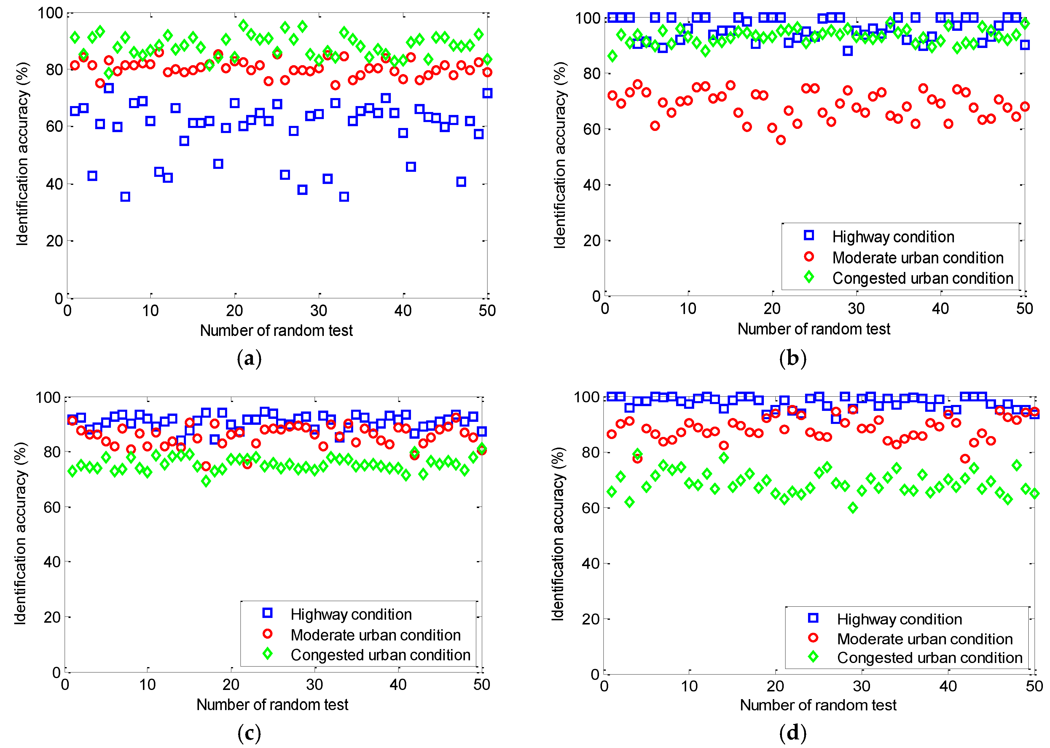
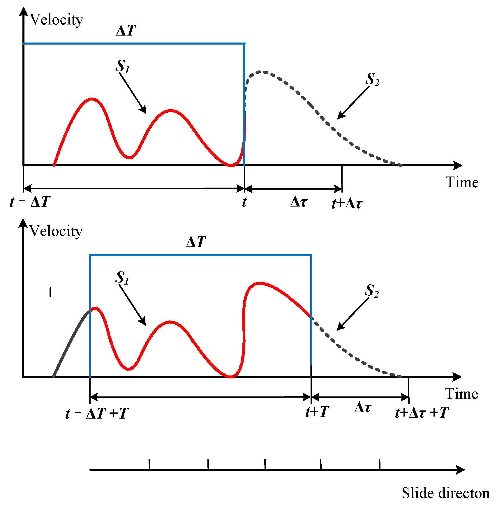
3.1.2. Slide Time Window Design

A slide time window is designed to extract characteristic parameters from driving cycles in a real time way. It is thus critical to ensure the network application for the onboard hybrid energy storage system in electric vehicles. The principle of the slide time window is shown in Figure 14.

Assume the current time is t, the length of time window is ΔT, and the sampling time is T, then the history driving cycle data S₁ in the time range from t – ΔT to t is used as the base data to identify future Δτ time range driving cycle S₂. At the next time point t – ΔT + T, new driving cycle data is added to the base data, and the history driving cycle data at time point t – ΔT is then given up, which is repeated and slide forward and thus referred to as slide time window. The part characteristic parameters extracted from three groups of driving cycles based on a 200 s slide time window are shown in Figure 15, Figure 16 and Figure 17.

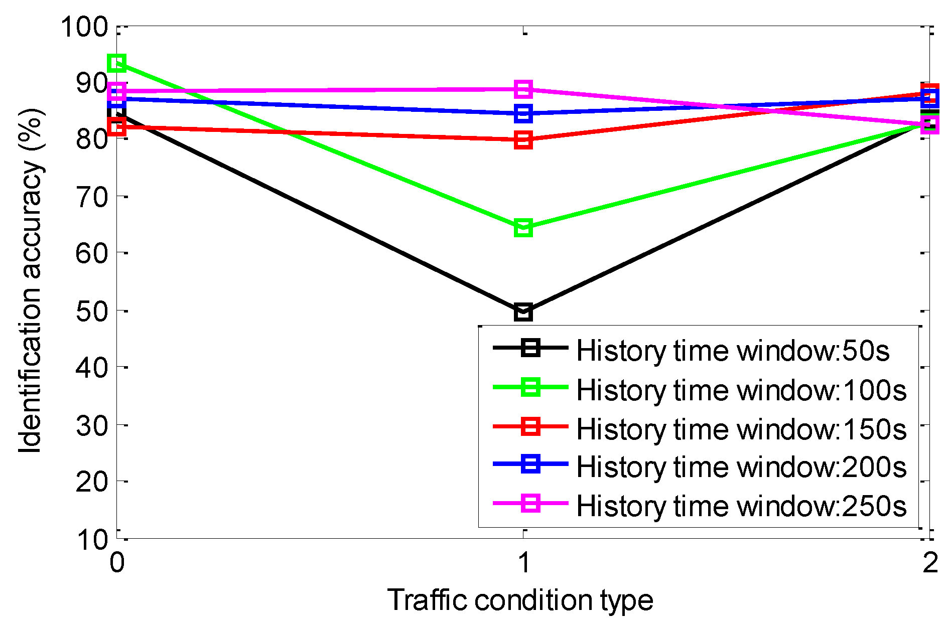
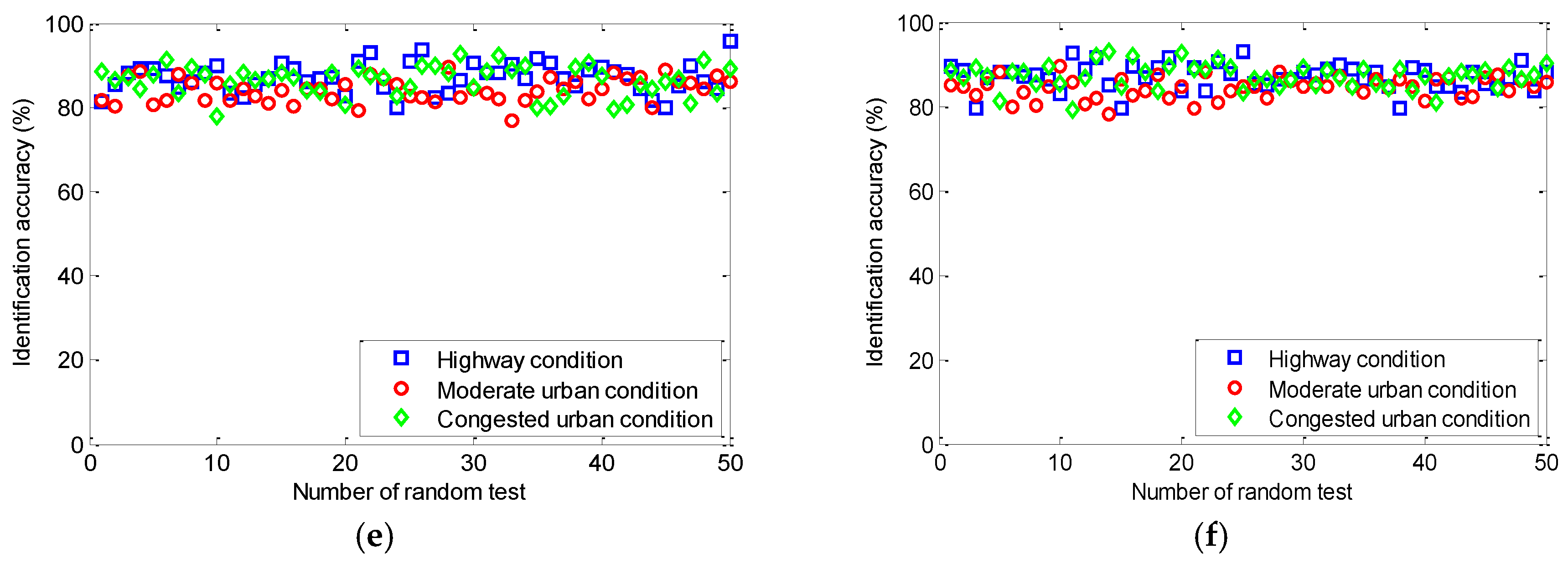
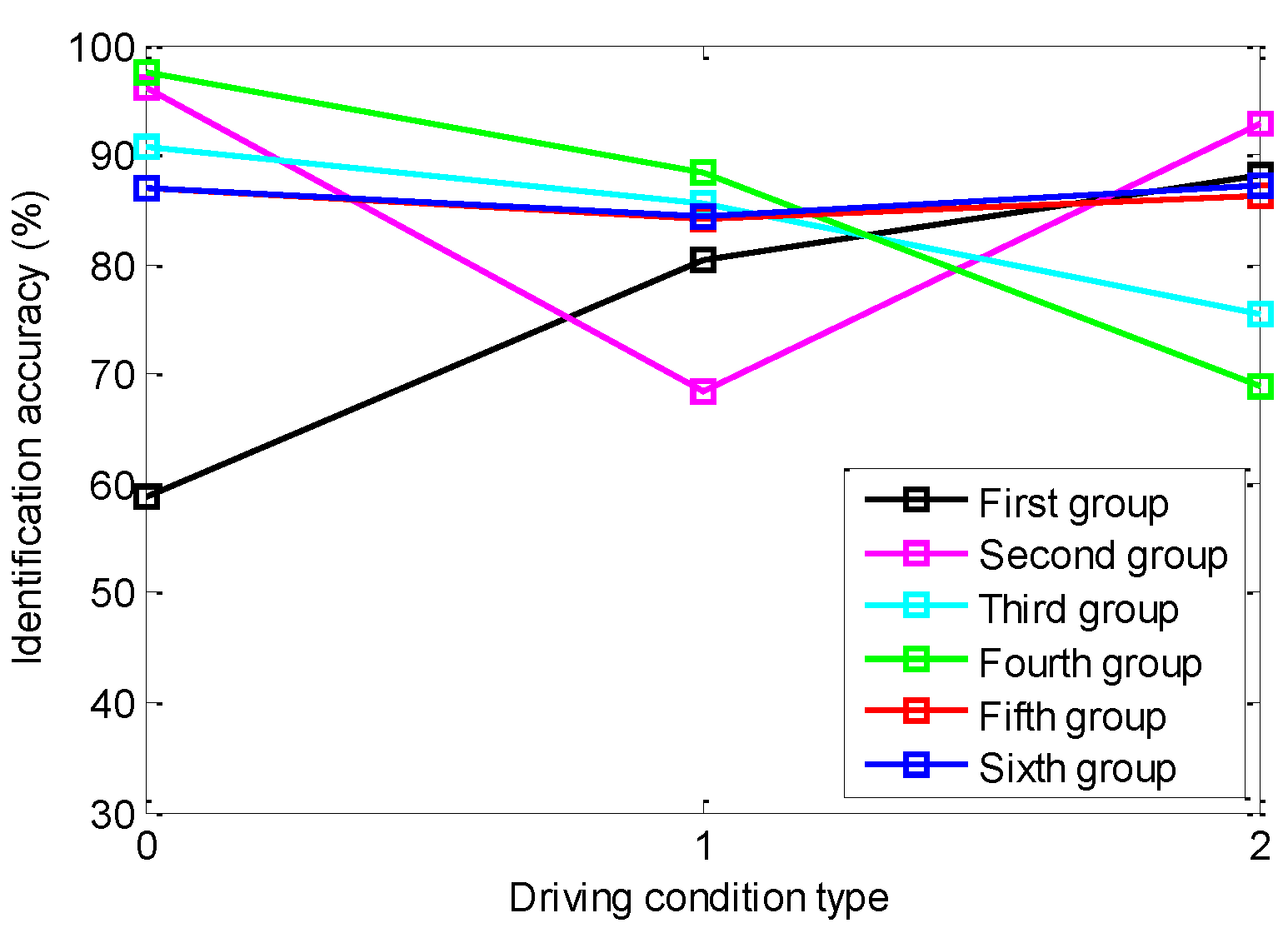
3.1.3. Optimal Slide Time Window Length

The length of the slide time window plays a very important role in trading off identification accuracy and time consumption. A longer slide time window will encompass superfluous history cycle information and yield a large time consumption, while a shorter slide time window could lead to a loss of useful information. Therefore, to achieve the optimal slide time window length, simulations and comparisons are carried out based on the 18 characteristic parameters described above.

Figure 18 shows the comparison results based on the length range of slide time window that varies from 50 s to 250 s; correspondingly, the results are superimposed in Figure 19. As is evident from Figure 19, the identification accuracy increases as the slide time window length increases, but when the slide time window length further increases to 250 s, the identification accuracy of the congested urban cycle cycles fails to increase rather decrease. Moreover, the identification accuracy of the highway cycle takes on a very slow growth trend. Weighing time consumption with the identification accuracy for each group of driving cycles, a 200 s slide time window length is finally determined.

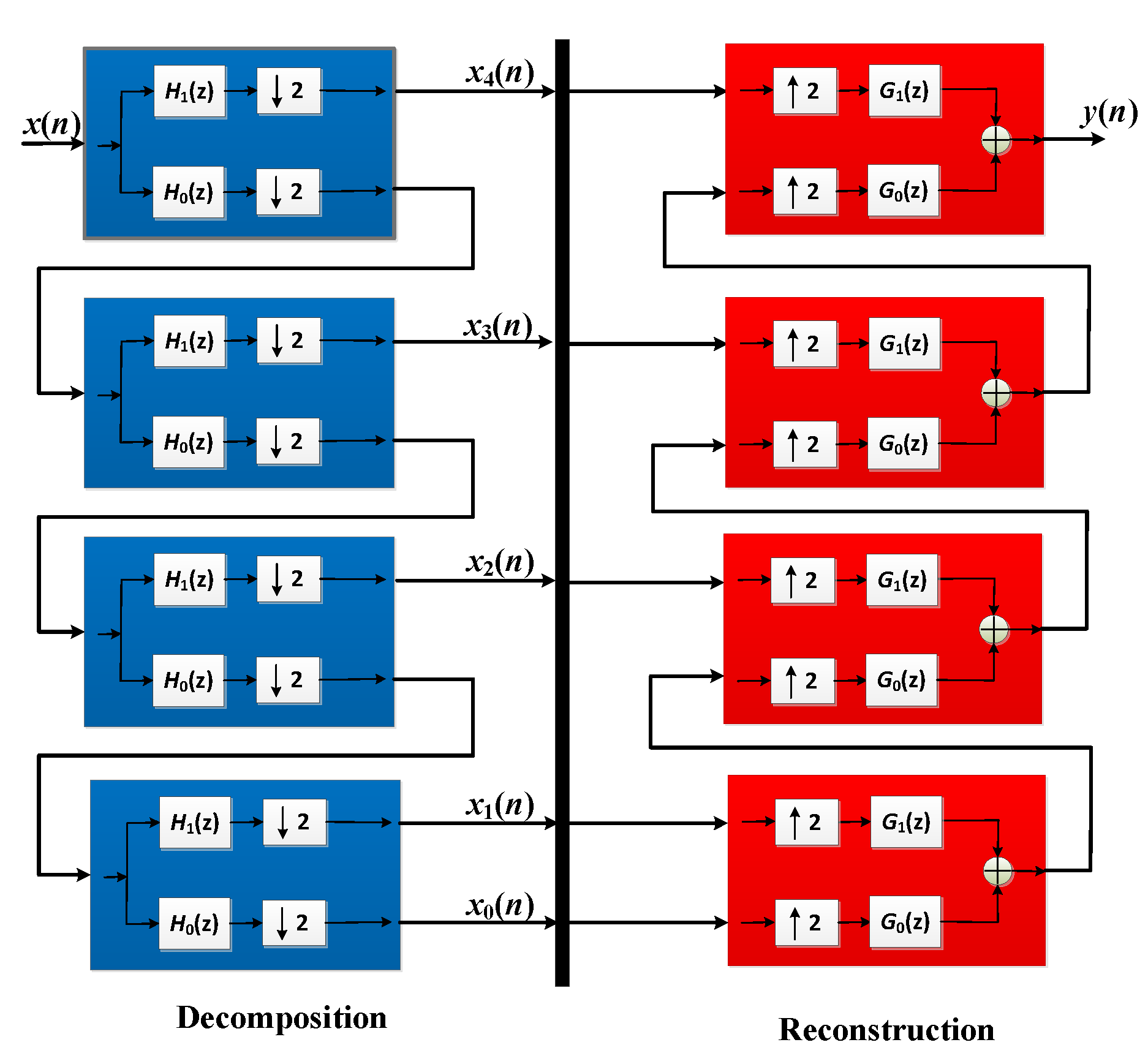
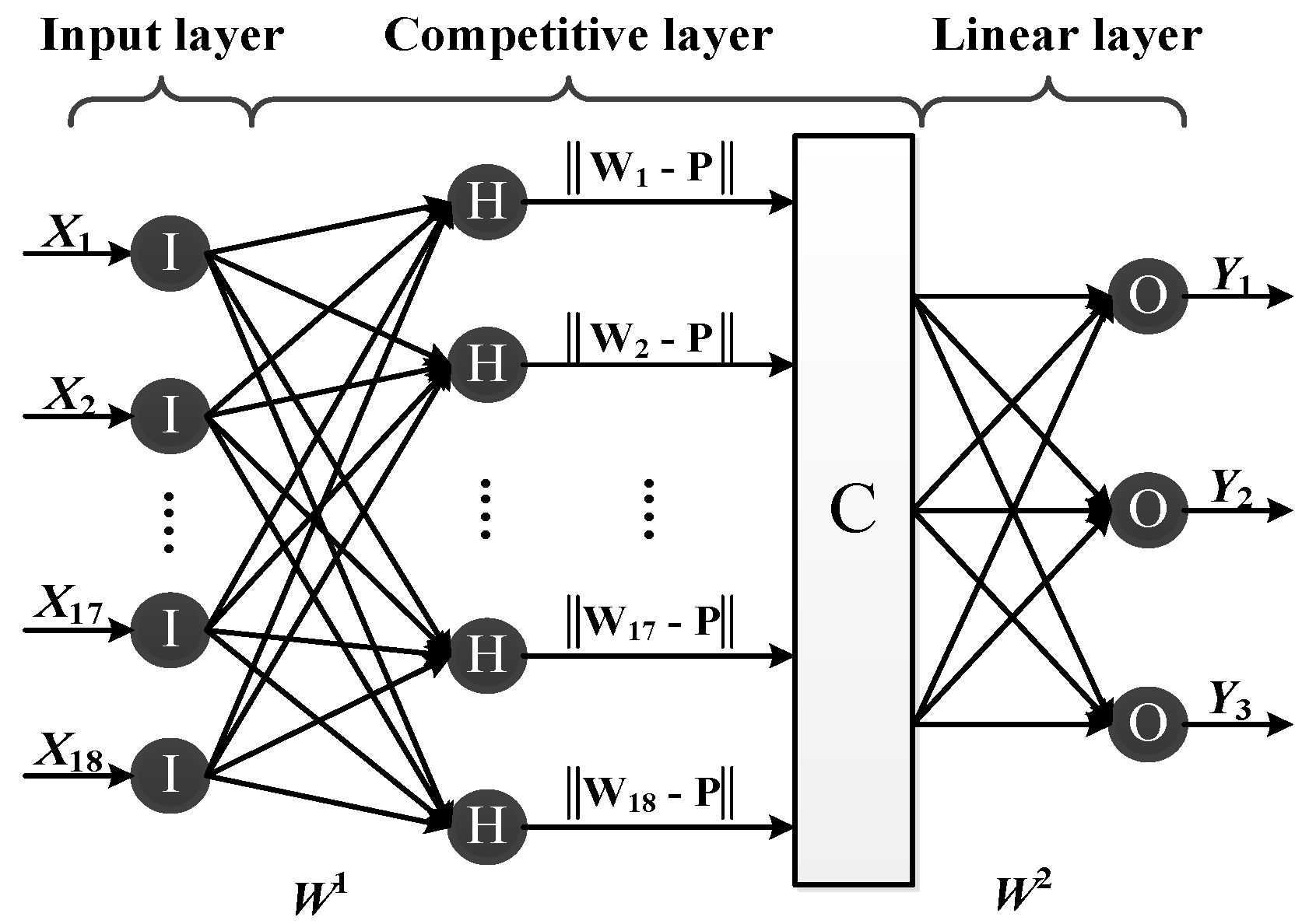
3.2. Harr-WT Algorithm

Since the cycle lifetime of an electric vehicle battery is typically less than two thousand times, frequent and deep charge-discharge processes will result in a sharp attenuation in battery cycle lifetime. In order to meet load power demand effectively while avoiding the rapid-variation and large-differential power demand for the battery, the application of frequency decoupled algorithms that extract the high-low frequency components from the total power demand based on the different dynamic characteristics consideration of battery and supercapacitor is quite essential for power management of the HESS. With regard to various frequency decoupling algorithms, wavelet transform (WT) is a relatively new and powerful tool in the analysis of the power transformer transient phenomenon because of its ability to extract information from the transient signals simultaneously in both the time and frequency domain by employing the long windows at low frequencies and short windows at high frequencies, rather than conventional Fourier Transform which can only give the information in the frequency domain [43,44,45]. Moreover, wavelet transform can narrow the correlation in different features tremendously and decomposes an original signal into components at different positions and scales with the smallest loss of important edge information compared to conventional filtering techniques [34]. Of all wavelets, the Haar wavelet has the shortest filter length in the time domain and is the simplest possible wavelet compared to other wavelets. Besides, it has the same characteristic between forward direction function and reverse direction function, which is a convenient application in signal process and improve the code execution efficiency. Therefore, the Haar wavelet transform algorithm is employed to determine the location of different frequency components in the load power demand.

Multi-level Haar-WT is applied for the load power decomposition, this is different from the prior research in Ref. [34,46], in which the level of Haar-WT for the load power decomposition is not discussed according to variations of the driving cycles. In this research, the decomposition level of Haar-WT is variable and finally determined according to the specific driving cycle type that identified by the LVQ neural network.

A four-level Haar-WT decomposition and reconstruction is shown in Figure 20. In the process of Haar wavelet decomposition, two filters, high pass filter H₁ and low pass filter H₀, are used to decompose the signal into high-low frequency components with the down-sampling methods. The data size reduces by half in down-sampling operations while it doubles in up-sampling operations. The high-low pass filters are combined with down-sampling operations, that is, steps that throw away every other sample at each process, reducing the data size by 50% each time [34,46]. In the same way of Haar wavelet decomposition, two filters, high pass filter G₁ and low pass filter G₀, are used to reconstruct the signal with the up-sampling operations for reconstruction.

The original signal $x\left(n\right)$ equals the predetermined load power demand. As shown in Figure 20, after four-level low-pass processing, the smooth slow-variation signal $x_0\left(n\right)$ is obtained as the power demand for the battery. Other transients ($x_1\left(n\right)+x_2\left(n\right)+x_3\left(n\right)+x_4\left(n\right)$) are distributed to the supercapacitor. This distribution method can be carried out for the highway driving cycle. As for two other driving cycles, the moderate urban cycle and the congested urban cycle, the three-level and two-level Haar-WT are assigned for frequency decomposition respectively. In this way, sudden peaks of power demand can be supplied the supercapacitor, whereas the high-low frequency variations of load power demand can be shared by supercapacitor and battery effectively. The specific power sharing method is expressed in Equations (15)–(17):

$$\{\begin{array}{c}{P}_{bat,1}=x_0\left(n\right)\\ P_{SC,1}=x_1\left(n\right)+x_2\left(n\right)+x_3\left(n\right)+x_4\left(n\right)\end{array}$$

(15)

$$\{\begin{array}{c}{P}_{bat,2}=x_0\left(n\right)\\ P_{SC,2}=x_1\left(n\right)+x_2\left(n\right)+x_3\left(n\right)\end{array}$$

(16)

$$\{\begin{array}{c}{P}_{bat,3}=x_0\left(n\right)\\ P_{SC,3}=x_1\left(n\right)+x_2\left(n\right)\end{array}$$

(17)

Based on this sharing strategy, the power demands for battery and supercapacitor can be adjusted flexibly and thus can better adapt to variations of driving cycles, which is a major advantage of the proposed energy management system. As a result, both system efficiency and battery lifetime can be further increased compared with the conventional sole frequency control. The frame of the proposed energy management system is shown in Figure 21.

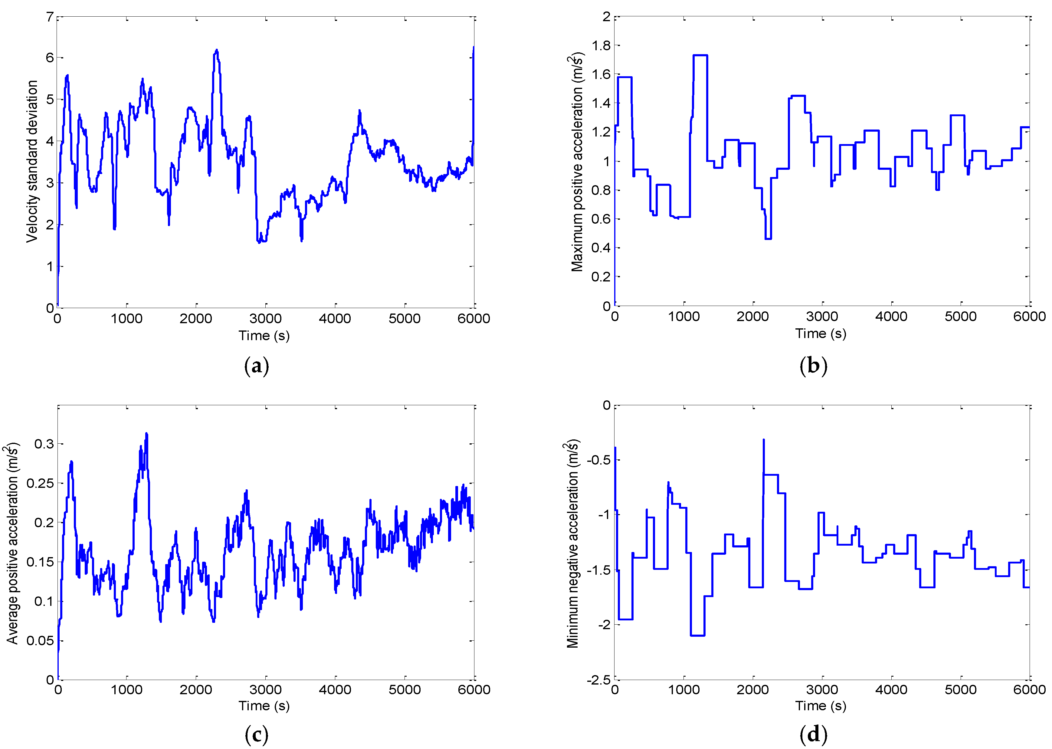
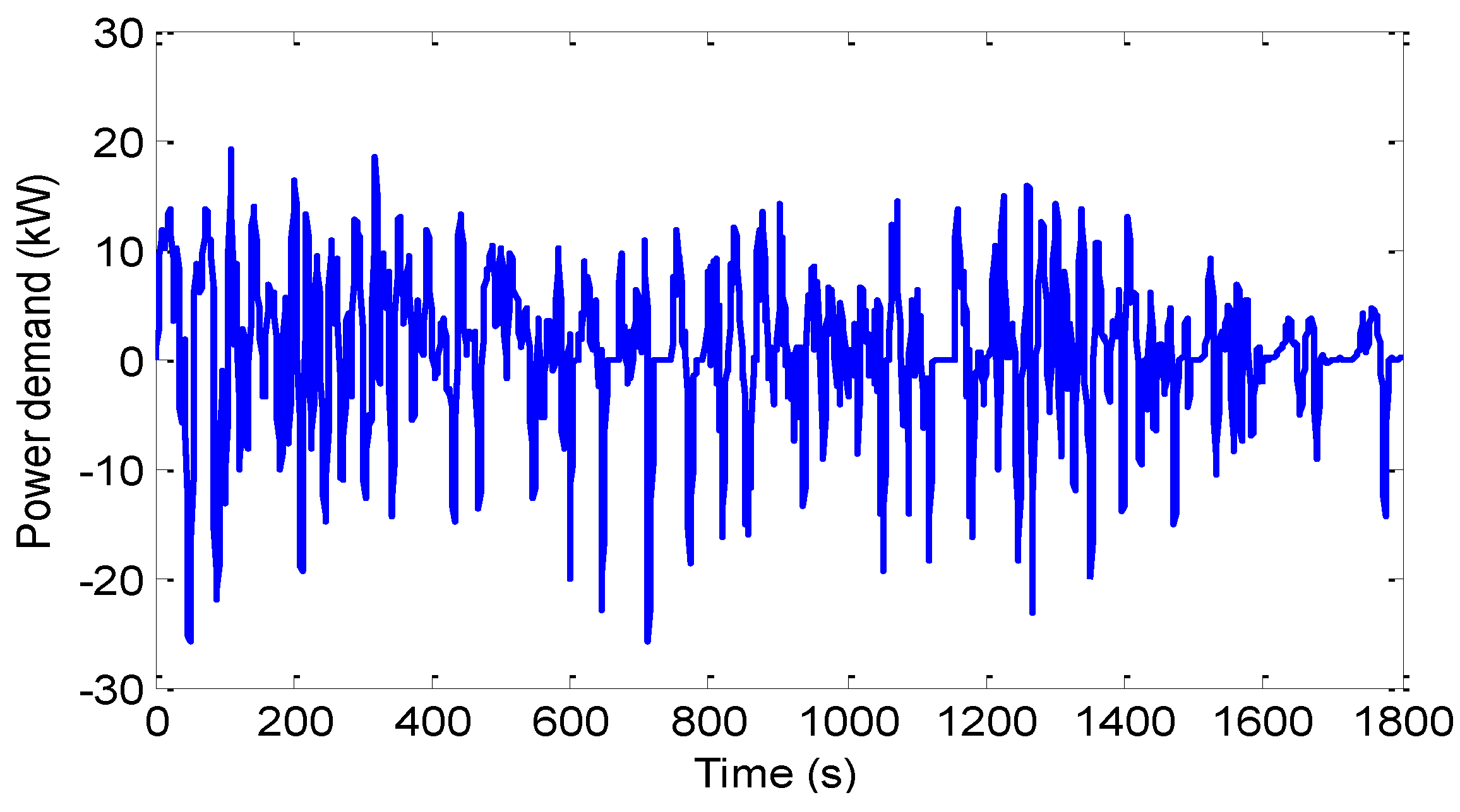
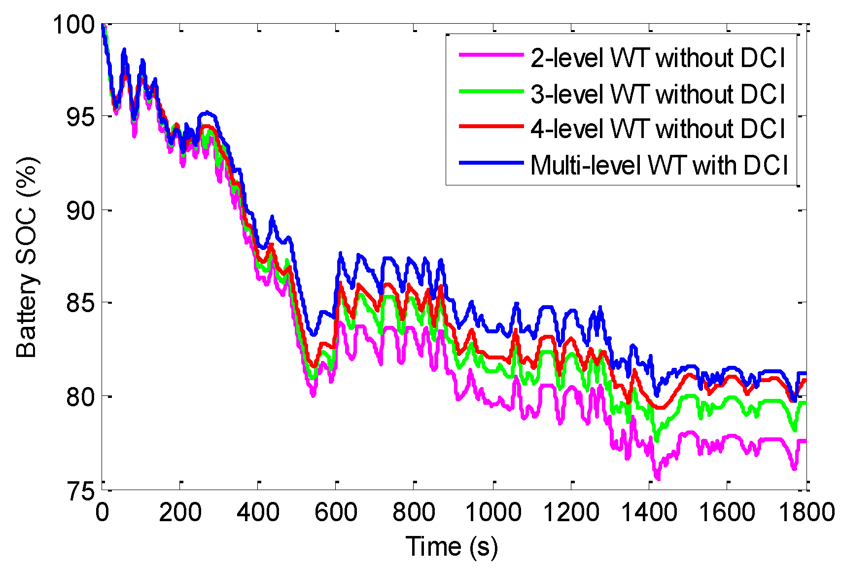
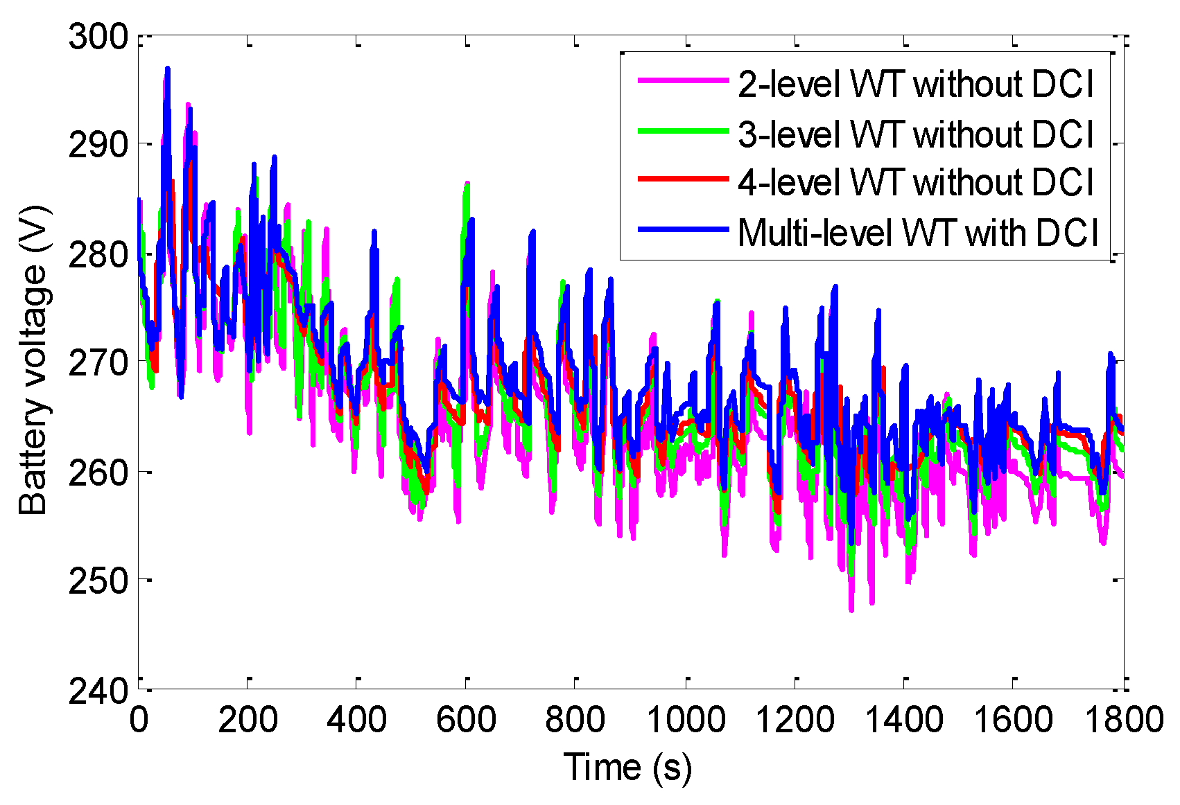
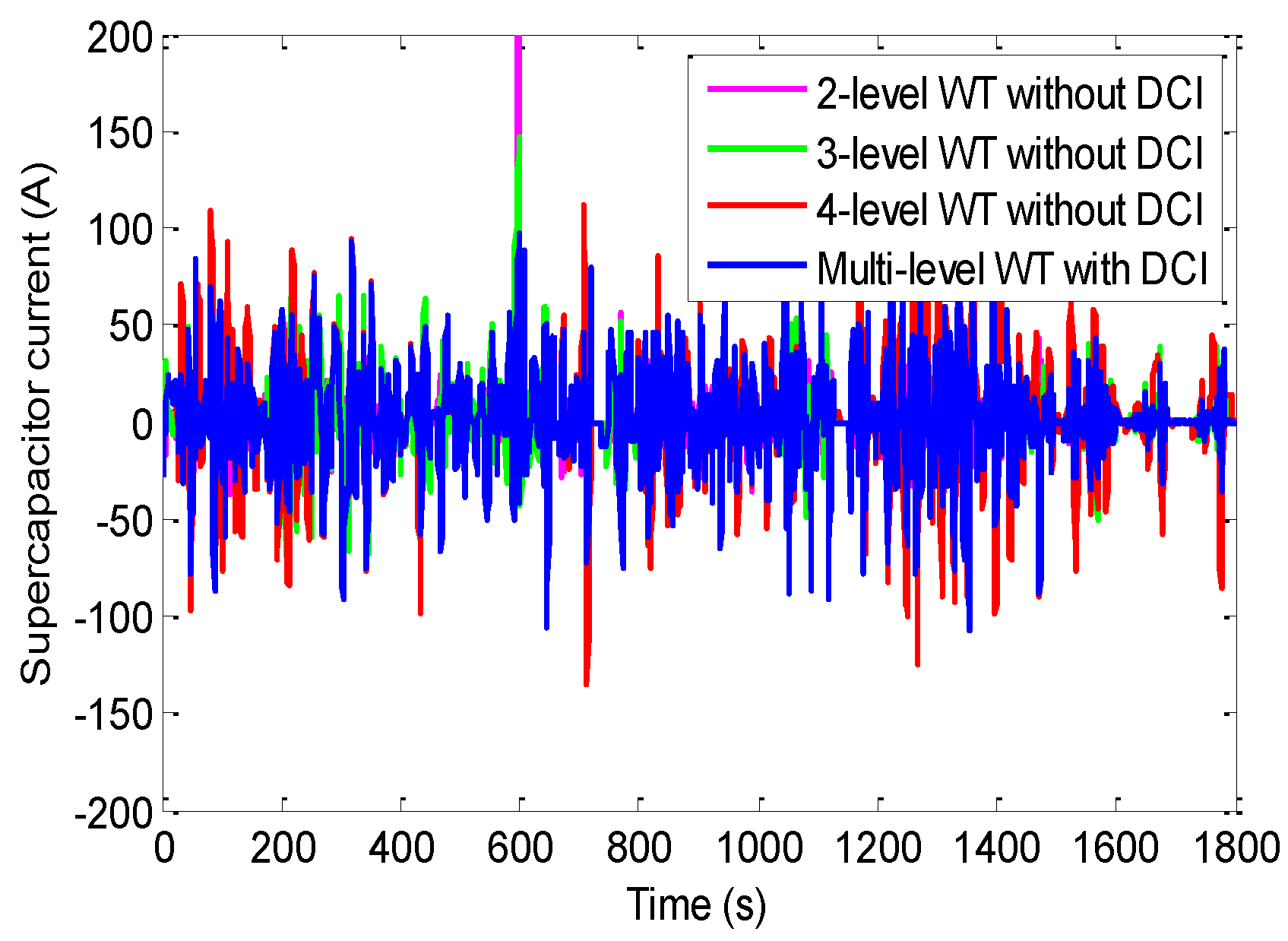
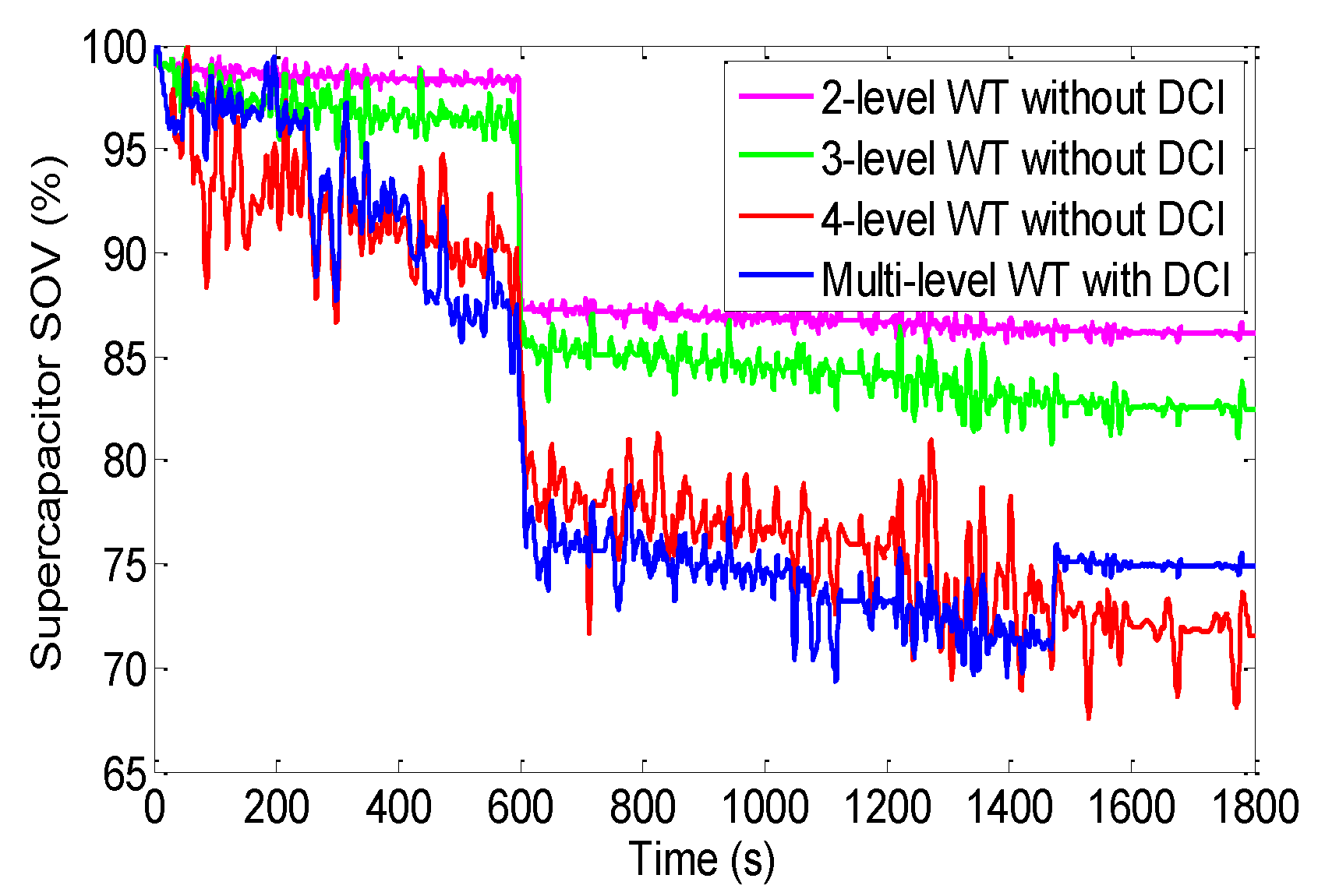
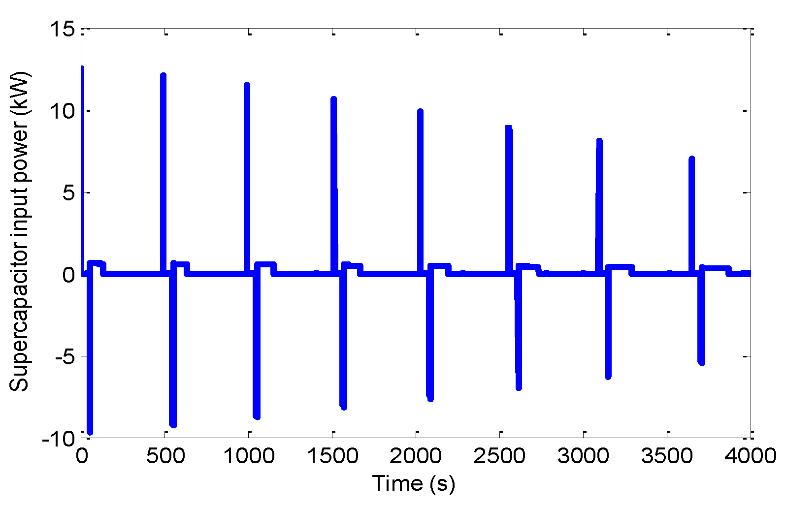
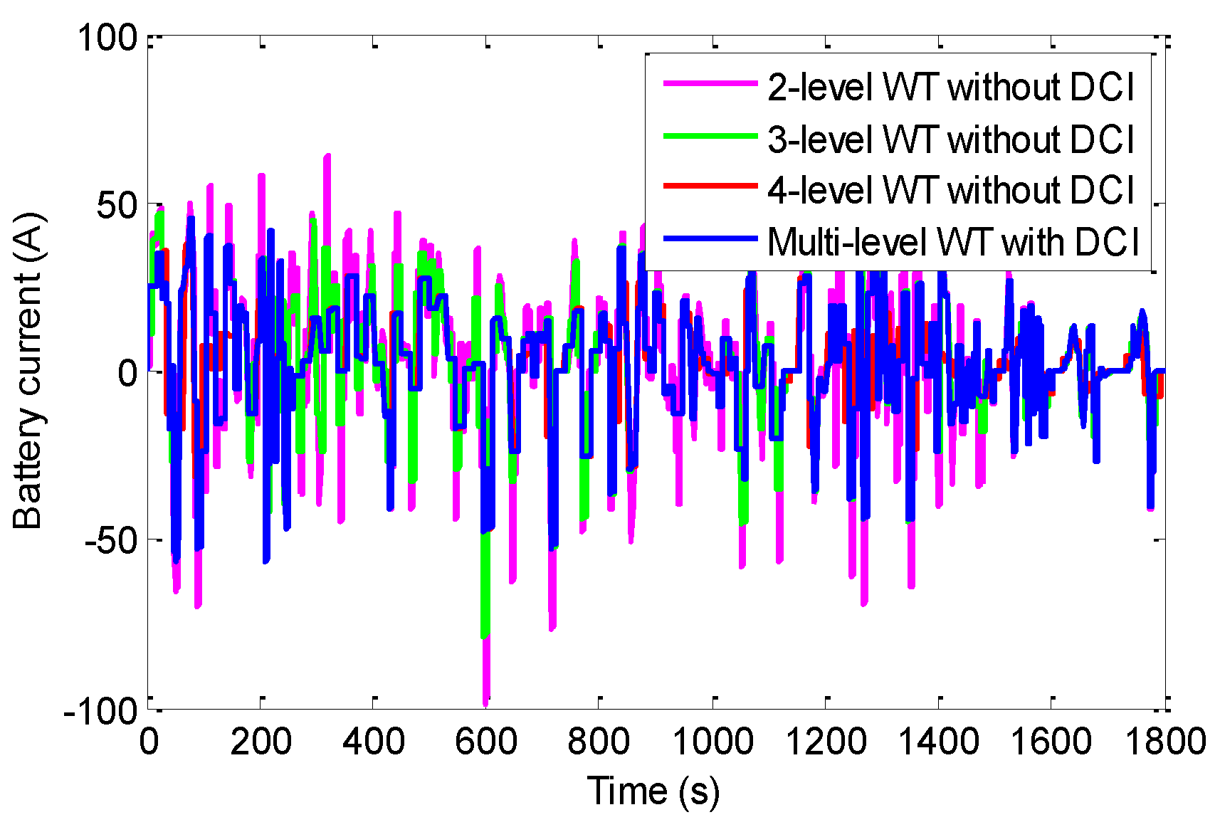
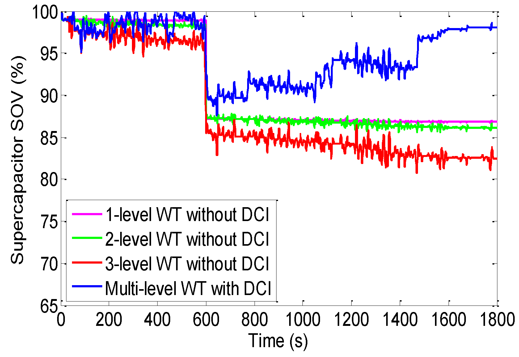
4. Results and Discussion

In order to evaluate the effectiveness of the proposed energy management system for HESS, a randomly generated driving cycle from the standard driving cycle library is used as the test cycle. The driving cycle is randomly generated from standard driving cycles accounting for an average 600 s time history for each standard driving cycle, which is shown in Figure 22. The power demand is calculated based on the test cycle with the main parameters of the tested electric vehicle that are listed in

Table 2. Main parameters of the tested electric vehicle.

Parameters Amount Unit
Mass 1550 kg
Frontal area 2.13 m2
Tire radius 0.3 m
Drag coefficient 0.36
Rolling resistance coefficient 0.02

, and the result is shown in Figure 23. The models of battery and supercapacitor are developed under MATLAB/Simulink environment based on the equivalent circuits, which have been shown in Figure 2 and Figure 5 respectively. The basic parameters of the simulated battery and supercapacitor used in this study are listed in

Table 3. Electrical parameters of the battery.

Parameters Amount Unit
Battery Type Lithium-ion battery
Nominal voltage 280 V
Nominal capacity 20 Ah
Number of cells 72

and

Table 4. Electrical parameters of the supercapacitor.

Parameters Amount Unit
Supercapacitor Type Maxwell BMO3000
Nominal voltage 140 V
Nominal capacity 55 F
Number of cells 55

, respectively.

Figure 24 shows the comparison results of the battery bank SoC with different controls. Since the proposed multi-level WT with DCI control can flexibly adjust different frequency components of load power between battery and supercapacitor based on the effective identification of the driving cycle, thus high frequency variations and sudden power demand peaks are successfully distributed to the supercapacitor. In this way, the supercapacitor is enabled to participate in the power share operation more frequently within the desired voltage range. As a result, the battery SoC consumption is greatly saved compared with other three controls, which should be very helpful to extend electric vehicle’s driving range. In addition, benefiting from the variable frequency distribution, the frequent charge and discharge operation for battery system is avoided, the battery’s power output is smoothed and thus battery system has much smaller SoC fluctuation. Consequently, the proposed method enables the battery system to satisfy charge/discharge operations of load power with shallow Depth of Discharge (DoD), which is beneficial to extending battery lifetime because the number of cycles to failure increases exponentially as DoD decreases.

Figure 25 represents the voltage comparison results of the battery bank. It can be clearly observed that there is a large voltage drop under the 4-level WT without DCI control and proposed multi-level WT with DCI control can be avoided compared to that of the other two controls, namely a good voltage stabilization performance can be obtained for the battery system. It can be seen that both the 4-level WT without DCI control and proposed multi-level WT with DCI control can maintain the voltage within the range from 255 V to 296 V, which is roughly estimated to be a maximum 41 V voltage drop compared with a maximum 48 V voltage drop for the other two controls. Therefore, for a 72 series battery cells, each cell assumes an average 0.57 V voltage fluctuation compared with 0.67 V voltage fluctuation. Therefore, it is obvious that the battery system is operated in much smaller voltage range and the potential battery cell balancing problem can be avoided to prevent individual cell voltages from a big drifting apart over time, which leads to rapid decreases of the total pack capacity, or even complete system failure.

The charging and discharging current of battery system under different controls is compared in Figure 26. It is clear that the 4-level WT without DCI control and proposed multi-level WT with DCI control can reduce the charging/discharging current largely compared to the other two controls, which would be very helpful to increase battery lifetime. Correspondingly, high frequency and large peak current are supplied by the supercapacitor, which is shown in Figure 27.

The SoV evolutions of the supercapacitor are illustrated in Figure 28. To guarantee effective power supply of the HESS, the SoV of supercapacitor bank should be maintained in reasonable fluctuation range. From Figure 28, it can be observed that the proposed WT with DCI control enable supercapacitor voltage to fluctuate largely while can successfully maintain supercapacitor voltage within suitable variation range compared with other controls, namely its fast response characteristic is utilized fully to fulfill the load power demand, thus the battery system’s working condition can be greatly optimized benefiting from the more frequent and effective participation of the supercapacitor. These operations would afford a beneficial protection for battery system from the aggressive transitions and sudden peaks in the load power demand.

The above results show that DCI based frequency separation can better ensure operation of the battery and supercapacitor within their individual unique frequency ranges, namely the low frequency components of the load power demand are distributed to the battery system, while the corresponding high frequency components are distributed to the supercapacitor system. The frequency separation is specifically designed according to the types of driving cycles. This is the unique advantage that the HESS can be utilized reasonably to share the load power demand with consideration of driving cycles. In this way, the load power distributed to battery and supercapacitor can be adjusted. As a result, the supercapacitor can be utilized reasonably and thus battery SoC can be saved. In addition, the supercapacitor voltage can be readily balanced by adjusting the combination of separation frequency which depends on the type of cycle. Namely, the WT decomposition level is adjusted according to possible regenerative energy supplied by each driving cycle. The tradeoff between driving energy and braking energy for each driving cycle can be analyzed effectively. A specific simulation is also carried out to shown the effectiveness of the proposed method, and the result is shown in Figure 29. Compared to sole frequency controls, it is obviously observed that the regenerative breaking is better utilized and supercapacitor has enough energy to supply the load peak demand at the next driving cycle even if a high acceleration power is required.

5. Conclusions

In this paper, a driving cycle identification-based frequency separation energy management system is proposed to overcome the problem that load power distributed to a battery and supercapacitor fail to be adjusted to adapt to variations of the driving cycle when the power sharing strategy is designed only based on a fixed frequency. The system is executed taking into account the influence of driving cycle on the power distribution and the driving cycle can be identified using a LVQ neural network method, which is assessed in both training and validation. Multi-level Haar wavelet transform is employed for decomposing the load power into different frequency components and the identification results are subsequently used to determine frequency components that distributed to battery and supercapacitor. In this way, the influence of driving cycle on the power distribution can be eliminated. In order to evaluate the performance of the proposed energy management system, computer simulation is carried out based on a randomly generated driving cycle from the standard driving cycle library. Compared with conventional sole frequency controls, the proposed energy management system can balance well the voltage of the supercapacitor by adjusting the combination of separation frequency and thus can ensure effective peak power supply by supercapacitor without over-discharging the supercapacitor. Consequently, both the system efficiency and potential battery lifetime are further increased. In future research work, a real system experiment setup will be designed to verify the effectiveness of the proposed energy management system.

References

1. Lukic, S.M.; Cao, J.; Bansal, R.C.; Rodriguez, F.; Emadi, A. Energy Storage Systems for Automotive Applications. IEEE Trans. Ind. Electron. 2008, 55, 2258–2267. [Google Scholar] [CrossRef]
2. He, H.-W.; Xiong, R.; Chang, Y.-H. Dynamic Modeling and Simulation on a Hybrid Power System for Electric Vehicle Applications. Energies 2010, 3, 1821–1830. [Google Scholar] [CrossRef]
3. Nelson, R.F. Power requirements for batteries in hybrid electric vehicles. J. Power Sources 2000, 9, 12–26. [Google Scholar] [CrossRef]
4. Chau, K.T.; Chan, C.C. Emerging energy-efficient technologies for hybrid electric vehicles. Proc. IEEE 2007, 95, 821–835. [Google Scholar] [CrossRef]
5. Rahimi-Eichi, H.; Ojha, U.; Baronti, F.; Chow, M.-Y. Battery management system—An overview of its application in the smart grid and electric vehicles. IEEE Ind. Electron. Mag. 2013, 7, 4–16. [Google Scholar] [CrossRef]
6. Khaligh, A.; Li, Z.; Emadi, A. Battery, ultracapacitor, fuel cell and hybrid energy storage systems for electric, hybrid electric, fuel cell, and plug-in hybrid electric vehicles: State-of-the-art. IEEE Trans. Veh. Technol. 2010, 59, 2806–2814. [Google Scholar] [CrossRef]
7. Tie, S.F.; Tan, C.W. A review of energy sources and energy management system in electric vehicles. Renew. Sustain. Energy Rev. 2013, 20, 82–102. [Google Scholar] [CrossRef]
8. Ren, G.Z.; Ma, G.Q.; Cong, N. Review of electrical energy storage system for vehicular applications. Renew. Sustain. Energy Rev. 2015, 41, 225–236. [Google Scholar] [CrossRef]
9. Pay, S.; Baghzouz, Y. Effectiveness of Battery-Supercapacitor Combination in Electric Vehicles. In Proceedings of 2003 IEEE Bologna Power Tech Conference, Bologna, Italy, 23–26 June 2003; pp. 728–733.
10. Schupbach, R.M.; Balda, J.C. The role of ultracapacitors in an energy storage unit for vehicle power management. In Proceedings of 2003 IEEE 58th Vehiclar Technology Conference (VTC2003-Fall), Orlando, FL, USA, 6–9 October 2003; pp. 3236–3240.
11. Ortuzar, M.; Moreno, J.; Dixon, J. Ultracapacitor-Based Auxiliary Energy System for an Electric Vehicle: Implementation and Evaluation. IEEE Trans. Ind. Electron. 2007, 54, 2147–2156. [Google Scholar] [CrossRef]
12. Guidi, G.; Undeland, T.; Hori, Y. Effectiveness of Supercapacitor as Power-Assist in Pure EV Using a Sodium-Nickel Chloride Battery as Main Energy Storage. In Proceedings of International Battery, Hybrid and Fuel Cell Electric Vehicle Symposium, Stavanger, Norway, 13–16 May 2009; pp. 13–16.
13. Gao, L.; Dougal, R.A.; Liu, S. Power enhancement of an actively controlled battery/ultracapacitor hybrid. IEEE Trans. Power Electron. 2005, 20, 236–243. [Google Scholar] [CrossRef]
14. Carter, R.; Cruden, A.; Hall, P.J. Optimizing for Efficiency or Battery Life in a Battery/Supercapacitor Electric Vehicle. IEEE Trans. Veh. Technol. 2012, 61, 1526–1533. [Google Scholar] [CrossRef]
15. Ruetschi, P. Aging mechanisms and service life of lead-acid batteries. J. Power Sources 2004, 127, 33–44. [Google Scholar] [CrossRef]
16. Lailler, P.; Zaninotto, F.; Nivet, S.; Torcheux, L.; Sarrau, J.-F.; Vaurijoux, J.-P.; Devilliers, D. Study of the softening of the positive active-mass in valve-regulated lead-acid batteries for electric-vehicle applications. Journal of Power Sources 1999, 78, 204–213. [Google Scholar] [CrossRef]
17. Omar, N.; Daowd, M.; Hegazy, O.; van den Bossche, P.; Coosemans, T.; van Mierlo, J. Electrical Double-Layer Capacitors in Hybrid Topologies—Assessment and Evaluation of Their Performance. Energies 2012, 5, 4533–4568. [Google Scholar] [CrossRef]
18. Ju, F.; Zhang, Q.; Deng, W.W.; Li, J.S. Review of structures and control of battery-supercapacitor hybrid energy storage system for electric vehicles. In Proceedings of the 2014 IEEE International Conference on Automation Science and Engineering (CASE), Taipei, Taiwan, 18–22 August 2014; pp. 18–22.
19. Kuperman, A.; Aharon, I. Battery/ultracapacitor hybrids for pulsed current loads: A re-view. Renew. Sustain. Energy Rev. 2011, 15, 981–992. [Google Scholar] [CrossRef]
20. Ortuzar, M.; Moreno, J.; Dixon, J. Ultracapacitor based auxiliary energy system for an electric vehicle: Implementation and evaluation. IEEE Trans. Ind. Electron. 2007, 54, 2147–2156. [Google Scholar] [CrossRef]
21. Onar, O.C.; Khaligh, A. A Novel Integrated Magnetic Structure Based DC/DC Converter for Hybrid Battery/Ultracapacitor Energy Storage Systems. IEEE Trans. Smart Grid 2012, 3, 296–307. [Google Scholar] [CrossRef]
22. Baisden, A.C.; Emadi, A. ADVISOR-Based Model of a Battery and Ultra-Capacitor Energy Source for Hybrid Electric Vehicles. IEEE Trans. Veh. Technol. 2004, 53, 199–205. [Google Scholar] [CrossRef]
23. Trovão, J.P.; Pereirinha, P.G.; Jorge, H.M.; Henggeler Antunes, C. A multi-level energy management system for multi-source electric vehicles–An integrated rule-based meta-heuristic approach. Appl. Energy 2013, 105, 304–318. [Google Scholar] [CrossRef]
24. Zhang, C.H.; Shi, Q.S.; Cui, N.X.; Li, W.H. Particle Swarm Optimization for energy management fuzzycontroller design in dual-source electric vehicle. In Proceedings of the IEEE Power Electronics Specialists Conference, Orlando, FL, USA, 17–21 June 2007; pp. 1405–1410.
25. Ates, Y.; Erdinc, O.; Uzunoglu, M.; Vural, B. Energy management of an FC/UC hybrid vehicular power system using a combined neural network-wavelet transform based strategy. Int. J. Hydrog. Energy 2010, 35, 774–783. [Google Scholar] [CrossRef]
26. Dusmez, S.; Khaligh, A. A supervisory power-splitting approach for a new ultracapacitor-battery vehicle deploying two propulsion machines. IEEE Trans. Ind. Inf. 2014, 10, 1960–1971. [Google Scholar] [CrossRef]
27. Martínez, J.S.; Hissel, D.; Pera, M.C.; Amiet, M. Practical control structure and energy management of a test bed hybrid electric vehicle. IEEE Trans. Veh. Technol. 2011, 60, 4139–4152. [Google Scholar] [CrossRef]
28. Hannan, M.A.; Azidin, F.A.; Mohamed, A. Multi-sources model and control algorithm of an energy management system for light electric vehicles. Energy Convers. Manag. 2012, 62, 123–130. [Google Scholar] [CrossRef]
29. Moreno, J.; Ortuzar, M.E.; Dixon, J.W. Energy-Management System for a Hybrid Electric Vehicle, Using Ultracapacitors and Neural Networks. IEEE Trans. Ind. Electron. 2006, 53, 614–623. [Google Scholar] [CrossRef]
30. Choi, M.-E.; Kim, S.-W.; Seo, S.-W. Energy Management Optimization in a Battery/Supercapacitor Hybrid Energy Storage System. IEEE Trans. Smart Grid 2012, 3, 463–472. [Google Scholar] [CrossRef]
31. Hredzak, B.; Agelidis, V.G.; Jang, M. A model predictive control system for a hybrid battery-ultracapacitor power source. IEEE Trans. Power Electron. 2014, 29, 1469–1479. [Google Scholar] [CrossRef]
32. Santucci, A.; Sorniotti, A.; Lekakou, C. Power split strategies for hybrid energy storage systems for vehicular applications. J. Power Sources 2014, 258, 395–407. [Google Scholar] [CrossRef]
33. Hredzak, B.; Agelidis, V.G.; Demetriades, G. Application of explicit mode predictive control to a hybrid battery-ultracapacitor power source. J. Power Sources 2015, 277, 84–94. [Google Scholar] [CrossRef]
34. Zhang, X.; Chris, C.T.M.; Masrur, A.; Daniszewski, D. Wavelet-transform-based power management of hybrid vehicles with multiple on-board energy sources including fuel cell, battery and ultracapacitor. J. Power Sources 2008, 185, 1533–1543. [Google Scholar] [CrossRef]
35. Kim, Y.; Lee, T.; Filipi, Z. Frequency domain power distribution strategy for series hybrid electric vehicles. SAE Int. J. Altern. Powertrains 2012, 1, 208–218. [Google Scholar] [CrossRef]
36. Chen, Z.; Li, L.; Yan, B.J.; Yang, C.; Marina Martínez, C.; Cao, D. Multimode energy management for plug-In hybrid electric buses based on driving cycles prediction. IEEE Trans. Transp. Syst. 2016, PP, 1–11. [Google Scholar] [CrossRef]
37. Hu, X.S.; Jiang, J.C.; Egardt, B.; Cao, D.P. Advanced power-source integration in hybrid electric vehicles: Multicriteria optimization approach. IEEE Trans. Ind. Electron. 2015, 6, 7847–7858. [Google Scholar] [CrossRef]
38. Lin, C.; Chou, B.; Chen, Q. Performance Comparison of battery power input equivalent circuit model for EVs. J. Chin. Automot. Eng. 2006, 28230–28234. [Google Scholar]
39. Spyker, R.L.; Nelms, R.M. Analysis of double-layer capacitors supplying constant power loads. IEEE Trans. Aerospace Electron. Syst. 2000, 36, 1439–1443. [Google Scholar]
40. Lin, C.C.; Jeon, S.; Peng, H.; Lee, J.M. Driving pattern recognition for control of hybrid electric trucks. Veh. Syst. Dyn. 2004, 42, 41–58. [Google Scholar] [CrossRef]
41. Langari, R.; Won, J.S. Intelligent energy management agent for a parallel hybrid vehicle-part I: System architecture and design of the driving situation identification process. IEEE Trans. Veh. Technol. 2005, 54, 925–934. [Google Scholar] [CrossRef]
42. He, H.; Sun, C.; Zhang, X. A method for identification of driving patterns in hybrid electric vehicles based on a LVQ neural network. Energies 2012, 5, 3363–3380. [Google Scholar] [CrossRef]
43. Mao, P.L.; Aggarwal, R.K. A Novel Approach to the Classification of the Transient Phenomena in Power Transformers Using Combined Wavelet Transform and Neural Network. IEEE Trans. Power Deliv. 2001, 16, 654–660. [Google Scholar] [CrossRef]
44. Capilla, C. Application of the Haar wavelet transform to detect micro-seismic signal arrivals. J. Appl. Geophys. 2006, 59, 36–46. [Google Scholar] [CrossRef]
45. Joseph, L.; Minh-Nghi, T. A wavelet-based approach for the identification of damping in nonlinear oscillators. Int. J. Mech. Sci. 2005, 47, 1262–1281. [Google Scholar] [CrossRef]
46. Erdinc, O.; Vural, B.; Uzunoglu, M. A wavelet-fuzzy logic based energy management strategy for a fuel cell/battery/ultra-capacitor hybrid vehicular power system. J. Power Sources 2009, 194, 369–380. [Google Scholar] [CrossRef]
Figure 1. Configuration of battery/supercapacitor hybrid system. DC, direct current.
Energies 09 00341 g001
Figure 2. PNGVs battery equivalent electric circuit. C b , open-voltage fluctuation; C p , polarization capacitance; I L , current; R 0 , ohm resistance; R p , polarization resistance; U b , fluctuation voltage of open-voltage; U L , voltage of the battery; U o c , ideal voltage source; U p , over-voltage; U 0 , ohm resistance voltage.
Energies 09 00341 g002
Figure 3. Battery charging/discharging power.
Energies 09 00341 g003
Figure 4. Voltage curve comparisons of the battery.
Energies 09 00341 g004
Figure 5. Supercapacitor equivalent electric circuit. C S C , capacitor;   R e p r , self-discharging loss; R e s r , charging/discharging resistance I L S C , load current of the supercapacitor; U L S C , load voltage of the supercapacitor; U S C , terminal voltage of the supercapacitor; U R , ohm resistance voltage.
Energies 09 00341 g005
Figure 6. Supercapacitor input charging/discharging power.
Energies 09 00341 g006
Figure 7. Voltage comparison curves of the supercapacitor.
Energies 09 00341 g007
Figure 8. Architecture of learning vector quantization (LVQ) neural network.
Energies 09 00341 g008
Figure 9. Six standard driving cycles. (a) is the INDIA_HWY_SAMPLE driving cycle; (b) is the HWFET driving cycle; (c) is the UDDS driving cycle; (d) is the WVUSUB driving cycle; (e) is the INDIA_URBAN_SAMPLE driving cycle; (f) is the UKBUS6 driving cycle.
Energies 09 00341 g009
Figure 10. Comparison histograms of part characteristic parameters.
Energies 09 00341 g010aEnergies 09 00341 g010b
Figure 11. Identification accuracy based on sole characteristic parameter.
Energies 09 00341 g011
Figure 12. Identification accuracy of six groups of characteristic parameters. (a) First group of characteristic parameters; (b) Second group of characteristic parameters; (c) Third group of characteristic parameters; (d) Fourth group of characteristic parameters; (e) Fifth group of characteristic parameters; (f) Sixth group of characteristic parameters.
Energies 09 00341 g012aEnergies 09 00341 g012b
Figure 13. Accuracy comparison of six groups of characteristic parameters.
Energies 09 00341 g013
Figure 14. Principle of the slide time window.
Energies 09 00341 g014
Figure 15. Characteristic parameters extracted from highway driving cycle. (a) Velocity standard deviation; (b) Maximum positive acceleration; (c) Average positive acceleration; (d) Minimum negative acceleration.
Energies 09 00341 g015
Figure 16. Characteristic parameters extracted from moderate urban driving cycle. (a) Velocity standard deviation; (b) Maximum positive acceleration; (c) Average positive acceleration; (d) Minimum negative acceleration.
Energies 09 00341 g016aEnergies 09 00341 g016b
Figure 17. Characteristic parameters extracted from congested urban driving cycle. (a) Velocity standard deviation; (b) Maximum positive acceleration; (c) Average positive acceleration; (d) Minimum negative acceleration.
Energies 09 00341 g017
Figure 18. Identification accuracy based on different length ranges of slide time window. (a) Identification accuracy with 50 s; (b) Identification accuracy with 100 s; (c) Identification accuracy with 150 s (d) Identification accuracy with 200 s; (e) Identification accuracy with 250 s.
Energies 09 00341 g018
Figure 19. Comparisons based on length range of slide time window that varies from 50 s to 250 s.
Energies 09 00341 g019
Figure 20. Principle of four-level Haar wavelet decomposition and reconstruction. H0 represents low pass filter of the Haar wavelet decomposition; H1 represents high pass filter of the Haar wavelet decomposition; G0 represents low pass filter of the Haar wavelet reconstruction; G1 represents high pass filter of the Haar wavelet reconstruction.
Energies 09 00341 g020
Figure 21. Frame of the proposed energy management system. DC, direct current; LVQ, learning vector quantization.
Energies 09 00341 g021
Figure 22. Randomly generated driving cycle from the standard driving cycle library.
Energies 09 00341 g022
Figure 23. Power demand of the test cycle.
Energies 09 00341 g023
Figure 24. State of charge (SoC) comparison of battery bank. WT, wavelet transform; DCI, driving cycle identification.
Energies 09 00341 g024
Figure 25. Voltage comparison of battery bank. WT, wavelet transform; DCI, driving cycle identification.
Energies 09 00341 g025
Figure 26. Current comparison of battery bank. WT, wavelet transform; DCI, driving cycle identification.
Energies 09 00341 g026
Figure 27. Current comparison of supercapacitor bank. WT, wavelet transform; DCI, driving cycle identification.
Energies 09 00341 g027
Figure 28. The state of voltage (SoV) comparison of supercapacitor bank. WT, wavelet transform; DCI, driving cycle identification.
Energies 09 00341 g028
Figure 29. The state of voltage (SoV) comparison by adjusting combination of wavelet transform (WT) decomposition level. DCI, driving cycle identification.
Energies 09 00341 g029