Article

Optimal Day-Ahead Scheduling of a Smart Distribution Grid Considering Reactive Power Capability of Distributed Generation

1
School of Electrical Engineering, Wuhan University, Wuhan 430072, China
2
School of Automation, Wuhan University of Technology, Wuhan 430070, China
*
Author to whom correspondence should be addressed.
Energies 2016, 9(5), 311; https://doi.org/10.3390/en9050311
Submission received: 3 March 2016 / Revised: 8 April 2016 / Accepted: 18 April 2016 / Published: 25 April 2016
(This article belongs to the Special Issue Microgrids 2016)

Abstract

:
In the traditional paradigm, large power plants provide active and reactive power required for the transmission system and the distribution network purchases grid power from it. However, with more and more distributed energy resources (DERs) connected at distribution levels, it is necessary to schedule DERs to meet their demand and participate in the electricity markets at the distribution level in the near future. This paper proposes a comprehensive operational scheduling model to be used in the distribution management system (DMS). The model aims to determine optimal decisions on active elements of the network, distributed generations (DGs), and responsive loads (RLs), seeking to minimize the day-ahead composite economic cost of the distribution network. For more detailed simulation, the composite cost includes the aspects of the operation cost, emission cost, and transmission loss cost of the network. Additionally, the DMS effectively utilizes the reactive power support capabilities of wind and solar power integrated in the distribution, which is usually neglected in previous works. The optimization procedure is formulated as a nonlinear combinatorial problem and solved with a modified differential evolution algorithm. A modified 33-bus distribution network is employed to validate the satisfactory performance of the proposed methodology.

1. Introduction

Global warming, energy crises, and ongoing serious environmental pollution have promoted the development of renewable energy greatly. With the benefit of low pollution and economic cost, they are encouraged to be used instead of fossil fuels. However, the high penetration of distributed energy resources (DERs) would pose a more complex operational situation for the distribution network [1]. Under the circumstances, it is significant to assure the reliable and secure operation of the distribution; additionally, the reasonable utilization of DERs is crucial to the sustainable development of renewable energies.
Over these years, the smart grid has been presented as a good notion to deal with the new problems accompanied by the integration of DERs. As the rapid development of intelligent electronic devices and information communication technology, the concept of the smart grid has been extended to the distribution level. In 2008, at the Conference International des Grands Reseaux Electriques (CIGRE), the active distribution network (ADN) was first put forward [2]. Different from the traditional network characterized with passivity and single-phase, the DGs and demand-side management programs, such as RLs connected in the ADN are online-controllable. The distribution management system (DMS), as the core of secure and economical operation of the distribution network, is responsible for the optimal operation scheme in the ADN, considering the participation of DERs.
Relevant research has been reported in recent years. A day-ahead operational scheduling paradigm for a distribution network has been presented in [3] where DGs are judiciously taken into consideration for their goodness factors. Results showed significant benefits in terms of reduced losses and cost savings. The authors in [4] have proposed a DMS algorithm to manage an ADN. The algorithm targets the minimization of the cost of system operation through the coordination of flexible network topology with the management of energy resources. In [5], a short-term energy resource scheduling methodology for a smart grid has been developed considering the intensive penetration of DGs and demand-response programs. The methodology aims at minimizing the operation costs and involves different anticipation times: day-ahead, hour-ahead, and 5-min-ahead. The authors in [6] have presented a comprehensive day-ahead operation model that includes network technical constraints and can participate in both energy and reserve markets. Considering the minimization of cost of all integrated DERs and the minimization of the voltage magnitude difference in all buses, a multi-objective paradigm has been proposed to determine the optimal solution of resource scheduling for a smart grid in [7]. The results have shown the importance of taking into account the reactive scheduling in the distribution network.
Although remarkable achievements have been obtained, the previous works generally ignore the pollutant emission and reactive power support capabilities of wind and solar power in the optimal resource scheduling of the smart grid. As atmospheric pollution and global warming have become one of the main critical environmental issues, the electrical industry, most of which use fossil energy as fuel, should make a contribution to environmental protection [8]. Thus, the emission ought to be considered in the distribution scheduling. Meanwhile, the authors in [9] have demonstrated the steady-state reactive power loading capability of doubly-fed induction generators (DFIG)-based wind turbines. The authors in [10] have achieved a significant reduction in losses by reasonable utilization of the wind farm reactive power capability. In [11], the reactive capability limits of different renewable DGs have been discussed and incorporated in the distribution system expansion planning strategy. A scheme for a reactive power market for DGs in the distribution network is presented in [12], where DGs are not only used to deliver active power, but also encouraged to take part in the reactive power support. Therefore, in the optimal scheduling of smart distribution grid, it is sensible to take advantage of the DGs’ reactive power capability, especially wind turbines (WT) and photovoltaics (PV), which are usually neglected.
Based on the preceding discussions, an intelligent scheduling program for DMS is presented in this paper. The proposed DMS targets to seek the optimal control of available active elements through the minimization of composite economic cost of distribution network. The composite cost consists of three components. The first is the operation cost, including the cost of purchasing power from the whole market, the cost of DG dispatches, and the cost of RL participations; the second is the emission cost, including pollutant cost of purchasing power and DG power; the third is the cost of network losses. Furthermore, the reactive power capabilities of WT and PV are analyzed; then they are wisely scheduled to settle the optimal reactive power dispatch of the ADN, as well as the conventional DG. The technical constraints of the whole system and the DERs integrated to the network are accommodated in the AC power flow fashion. A modified differential evolution algorithm (MDE) is adopted to resolve the proposed program. The obtained results are investigated to assess the effect of proposed DMS on the technical and economical improvements.
The rest of this paper is organized as follows. After the introductory section, Section 2 addresses the reactive power capabilities of different DG systems integrated in the distribution system. Section 3 presents the proposed scheduling framework. Section 4 focuses on the optimization technique. Section 5 carries out several test cases and discusses the numerical results. Finally, Section 6 concludes the paper.

2. Reactive Power Capabilities of Different DG Systems

In the paper, the wind systems based on doubly-fed induction generators (DFIGs), PV systems are based on voltage source inverters (VSI), and diesel generators are considered as the DERs that are integrated to the distribution. The static reactive power capabilities of the different DERs are discussed as follows.

2.1. Wind System

DFIG can adjust its reactive power injection or absorption and maintain the maximum active power output at the same time. The maximum reactive power injection of the DFIG-based wind system is mainly limited by the maximum rotor current I n r , active power output P n , st WT and slip s n [13], which is expressed as:
Q n , st WTin = 3 | V n s | 2 χ n s + ( 3 χ n m χ n s V n s I n r ) 2 ( P n , st WT 1 s n ) 2
where Q n , st WTin is the maximum reactive power injection limit of the WT at bus n over a system state st; V n s is the stator voltage of the WT at bus n; χ n s is the stator reactance; χ n m is the magnetizing reactance.
The maximum reactive power absorption Q n , st WTab is determined by the steady-state stability limits [13], which is expressed as:
Q n , st WTab = 3 | V n s | 2 χ n s

2.2. PV System

The active power output of the VSI-based PV system depends on the light intensity, and the reactive power output can be independently controlled by the power angle and modulation index [14]. The maximum reactive injection Q n , st PVin and absorption Q n , st PVab is expressed as:
Q n , st PVin , Q n , st PVab = ± ( S n , st i p v ) 2 ( P n , s t PV )
where S n , st i p v is the rated apparent power of the inverter; P n , s t PV is the active power injection of the PV system.

2.3. Diesel Generator

A diesel generator (DE) is based on the traditional synchronous machine. The reactive power capability is controlled by the field excitation while maintaining stable active power output. The maximum reactive power injection Q n , st D E i n 1 and absorption Q n , st D E a b are limited by the maximum stator current I n s [15], which can be calculated by:
Q n , st D E i n 1 , Q n , st D E a b = ± ( | V n , st | I n s ) 2 ( P n , st DE ) 2
where V n , st is the system voltage at bus n; P n , st DE is the active power injection of DE.
The maximum reactive injection Q n , st D E i n 2 is also limited by the maximum rotor voltage E n r [15].
Q n , st DEin 2 = | V n , st | 2 X n d + ( | V n , st | E n r X n d ) 2 ( P n , s t DE ) 2
where X n d is the direct axis component of synchronous reactance.

3. The Proposed Scheduling Framework

In this section, a mathematical model for DMS is presented to seek the optimal scheduling of the purchasing power from the whole market, and make decisions on DERs options including DEs, WTs, PVs, and RLs. The proposed scheme schedules the available control variables of ADN in a 24 h day-ahead time horizon.

3.1. Objection Function

In addition to the economic benefit, the impacts of environment pollution and technology revenue are also considered in the scheduling framework. Thus, the composite economic cost of distribution network F ( x , u ) including operation cost F 1 ( x , u ) , emission cost F 2 ( x , u ) , and network loss cost F 3 ( x , u ) are proposed to be the objective function. That is:
Minimize   F ( x , u ) = F 1 ( x , u ) + F 2 ( x , u ) + F 3 ( x , u )
where x and u respectively denote the vectors of control and dependent variables. In Equation (7), P Grid , Q Grid are vectors of the active and reactive power from the whole market; P DG , Q DG are vectors of conventional DG (here, the DE) active and reactive power dispatches; Q WT is the vector of WT reactive power scheduling; Q PV is the vector of PV reactive power scheduling; P RL , Q RL are vectors of RL participations. In Equation (8), V is the vector of bus voltages; S f is the vector of apparent power flow of feeder f.
x = [ P Grid , Q Grid , P DG , Q DG , Q WT , Q PV , P RL , Q RL ]
u = [ V , S f ]

3.1.1. Operation Cost F1(x, u)

The distribution operation cost is composed of several terms. The first term is the cost of purchasing power from the day-ahead wholesale market; the second term is DG start-up and shut-down costs; the third term is DG fuel consumption cost and maintenance cost; the fourth term is the maintenance cost for WTs and PVs; and the fifth term is cost of RLs participations. WTs and PVs are powered by renewable energy, so its fuel costs can be ignored. Therefore, the operation cost is expressed as:
F 1 ( x , u ) = t T { i N S ρ Gird , t P Gird , i , t + i N D G X i , t S U DG , i + i N D G ( a i P DG , i , t 2 + b i P DG , i , t + c i ) + i N D G Z i , t S D DG , i + i N D G ρ DG , i , t P DG , i , t + i N W T ρ WT , i , t P WT , i , t + i N P V ρ PV , i , t P PV , i , t + i N R L ρ RL , i , t P RL , i , t } × Δ t
where t, T are index and set of time intervals, respectively; N S , N D G , N W T , N P V and N R L are respectively sets of substations, DGs, WTs, PVs, and RLs. ρ Gird is the day-ahead wholesale electricity price; S U DG , S D DG are DG start-up and shut-down costs; X, Z are binary variables for DG start-up and shut-down status; a, b, c are fuel cost function coefficients of DGs; ρ DG , ρ WT , ρ PV are maintenance cost coefficients of DGs, WTs, and PVs; P WT , P PV are active power output of WTs and PVs; ρ RL is the contract price of RLs participation.

3.1.2. Emission Cost F2(x, u)

The wholesale power is considered to be thermal power. Carbon dioxide (CO2), sulfur dioxide (SO2), and nitrogen oxide (NOx) are the main pollutants accompanied with the purchasing power and DGs power. WTs and PVs are deemed to be non-polluting. Thus, the emission cost is:
F 2 ( x , u ) = t T { i N S j M α j E j P Grid , i , t + i N D G j M α j F i , j P DG , i , t } × Δ t
where M is set of pollutant species; α j is emission coefficient of pollutant j, $/kg; E j is emission rate of pollutant j for thermal power, kg/MW; F i , j is emission rate of pollutant j for ith DG, kg/MW. In Equation (10), the first term is emission cost for the purchasing power from whole market; the second term is emission cost for DGs dispatches.

3.1.3. Network Loss Cost F3(x, u)

The active power loss of distribution network can be calculated by power flow. The cost is:
F 3 ( x , u ) = t T ρ l o s s , t P l o s s , t × Δ t
where ρ l o s s , t is unit cost of active power loss at time interval t, $/MW; P l o s s , t is active power loss of distribution at time interval t.

3.2. Constraints

3.2.1. Load Flow Equations Constraint

i N S P Grid , i + i N D G P DG , i + i N W T P WT , i + i N P V P PV , i + i N R L P R L , i i N n o d e P D , i = i N n o d e j N O | V i | | V j | | Y i j | cos ( δ j δ i + θ i j )
i N S Q Grid , i + i N D G Q DG , i + i N W T Q WT , i + i N P V Q PV , i + i N R L Q R L , i i N n o d e Q D , i = i N n o d e j N O | V i | | V j | | Y i j | sin ( δ j δ i + θ i j )

3.2.2. Purchasing Power Constraint

P Grid , i , t 2 + Q Grid , i , t 2 S Grid , i max i N S

3.2.3. WTs and PVs Limits

P WT , i min P WT , i , t P WT , i max i N W T
Q WT , i , t min Q WT , i , t Q WT , i , t max i N W T
P PV , i min P PV , i , t P PV , i max i N W T
Q PV , i , t min Q PV , i , t Q PV , i , t max i N W T

3.2.4. DG Generations Limits

P DG , i min P DG , i , t P DG , i max i N D G
Q DG , i , t min Q DG , i , t Q DG , i , t max i N D G
P DG , i , t + 1 P DG , i , t R R i i N D G
P DG , i , t P DG , i , t + 1 R R i i N D G

3.2.5. RL Constraints

0 P RL , i , t P RL , i max i N R L
Q RL , i , t = tan ( cos 1 ( P F RL , i ) ) × P RL , i , t i N R L

3.2.6. Steady-State Security Constraints

V i min V i , t V i max i N n o d e
S f S f max f N f
In these constraints, P D , Q D are, respectively, active and reactive power loads in each bus; V i , V j are voltage amplitudes of buses i and j; N n o d e is set of system buses; N O is the set of system buses, excluding bus i; Y i j is the admittance between bus i and j; δ i , δ j are voltage phases of buses i and j; θ i j is phase of Y i j . S Grid is the substation apparent power capacity; the superscripts “max” and “min” respectively denote the corresponding upper and lower limits. RR is ramping capability of DG. P F RL is constant power factor for RLs. N f is set of distribution feeders. In Equations (16), (18), and (20), the reactive power limits of WTs, PVs, and DGs should be associated with their steady-state characteristics as discussed in Section 2.

4. Optimization Technique

The proposed day-ahead optimal scheduling framework is a nonlinear combinatorial optimization problem. In this paper, a modified differential evolution (MDE) algorithm is presented to solve it. The differential evolution algorithm (DE) was first put forward by Storn and Price [16]. Its principle is simple and it is easy to be understood and implemented with fewer controlled parameters. DE has been used to solve different engineering optimization problems and achieved good effects [17,18,19,20]. However, the control parameters in DE have a great effect on the algorithm performance and their appropriate values must be obtained through numerous tests.

4.1. Original Differential Evolution Algorithm

DE is a kind of population-based algorithm, which can remember the best solutions and share the information within the population. Supposing the population size is N, the ith individual at Gth iteration can be expressed as X i , G ( i = 1 , 2 , , N ) . Then a new population is generated through mutation, crossover, and selection operation [16].
For each individual X i , G , three different individual vectors are randomly selected from the current iteration G; then the mutation vector V i , G + 1 can be produced by:
V i , G + 1 = X r 1 , G + F × ( X r 2 , G X r 3 , G )   r 1 r 2 r 3 i
where F is a scaling factor, which scales the difference vector ( X r 2 , G X r 3 , G ) . The trial vector U i , G + 1 is generated by crossover operator between the target vector X i , G and the mutation vector V i , G + 1 .
U i , G + 1 j = { V i , G + 1 j rand ( j ) CR   or   j = i rand X i , G j otherwise
where j [ 1 , 2 , , D ] , D is the dimension of the individual vector; rand(j) is a uniform random number within [0,1]; i rand is a random integer within [ 1 , 2 , , D ] . CR is the crossover rate. After mutation, the selection operator is performed to select the next generation, which is expressed as:
X i , G + 1 = { U i , G + 1 f ( U i , G + 1 ) f ( X i , G ) X i , G f ( U i , G + 1 ) > f ( X i , G )

4.2. Modified Differential Evolution Algorithm

4.2.1. Self-Learning Parameters Strategy

In original DE, all individuals in the population use the same F and CR, and their values remain unchanged in the evolution. Additionally, if the optimization problem is different, the values of F and CR should be reset. In order to make the parameters selection independent of optimization problems and improve the robustness of DE, a parameter self-learning strategy is proposed. In the strategy, the scaling factor F and crossover rate CR participates in individual coding and each individual X i , G corresponds to one F i , G and CR i , G . When initialized, F i , 0 and CR i , 0 are randomly generated within a given range.
In the evolution process, if an individual has not yielded one better child in successive m iterations, such as m = 5, it can be considered that the current control parameters of the individual is not appropriate, and should be reset; conversely, if an individual has yielded one or more better children in each successive m iterations, it can be considered that the current control parameters of the individual is appropriate, and should be retained. Thus, it is defined that in each successive n iterations, such as n = 10, the individual that has yielded the most, better, children is the “local optimal individual” and its corresponding control parameters are the “local optimal parameters”. Furthermore, in the current Gth iteration, the individual that has yielded the most, better, child individuals is the “global optimal individual” and its corresponding control parameters are the “global optimal parameters” in the current population. The inappropriate individual control parameters should learn from the “local optimal parameters” and “global optimal parameters” in the current population when reset. Thus, a self-learning parameters modification strategy is proposed.
F k , G + 1 = F k , G + w × ( 1 C k , l C l + 1 ) ( F l F k , G ) + ( 1 w ) × ( 1 C k , G C g + 1 ) ( F g F k , G )
CR k , G + 1 = CR k , G + w × ( 1 C k , l C l + 1 ) ( CR l CR k , G ) + ( 1 w ) × ( 1 C k , G C g + 1 ) ( CR g CR k , G )
where k is the number of the individual whose control parameters need to be reset; C k , l and C l are, respectively, the cumulative improvement times of the individual X k and the “local optimal individual” in successive n iterations; C k , G and C g are, respectively, the cumulative improvement times of the individual X k and the “global optimal individual” in the current Gth iteration; F l and CR l are the “local optimal parameters”; F g and CR g are the “global optimal parameters”; w is the weight factor which is equal to 0.5 here; ( 1 C k , l C l + 1 ) and ( 1 C k , G C g + 1 ) are named as the learning step. It can be seen that, for an individual, the smaller the cumulative improvement times is, the larger the learning step is, namely learning more from the “local optimal parameters” and “global optimal parameters”. Therefore, memory and information exchange functions are added to the proposed parameters modification strategy and the strategy has the ability of self-learning.

4.2.2. Boundary Handling
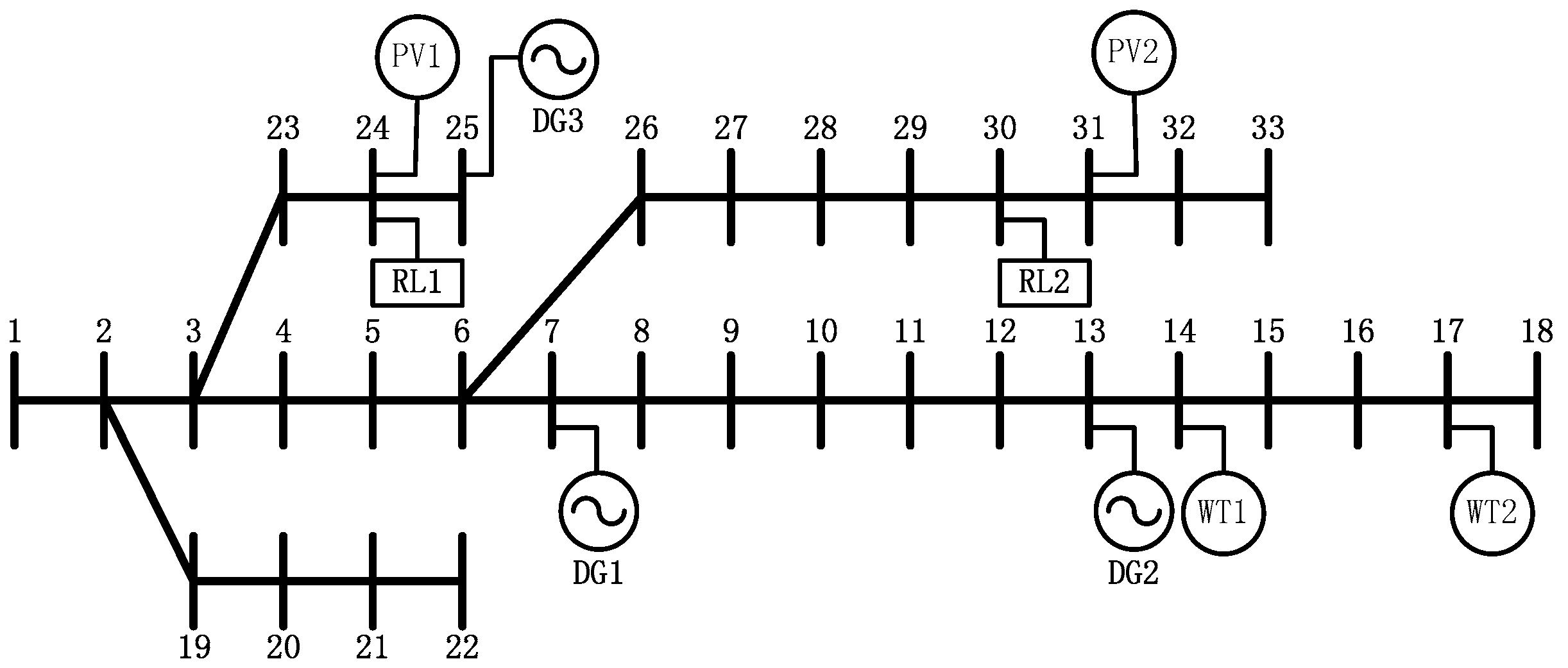
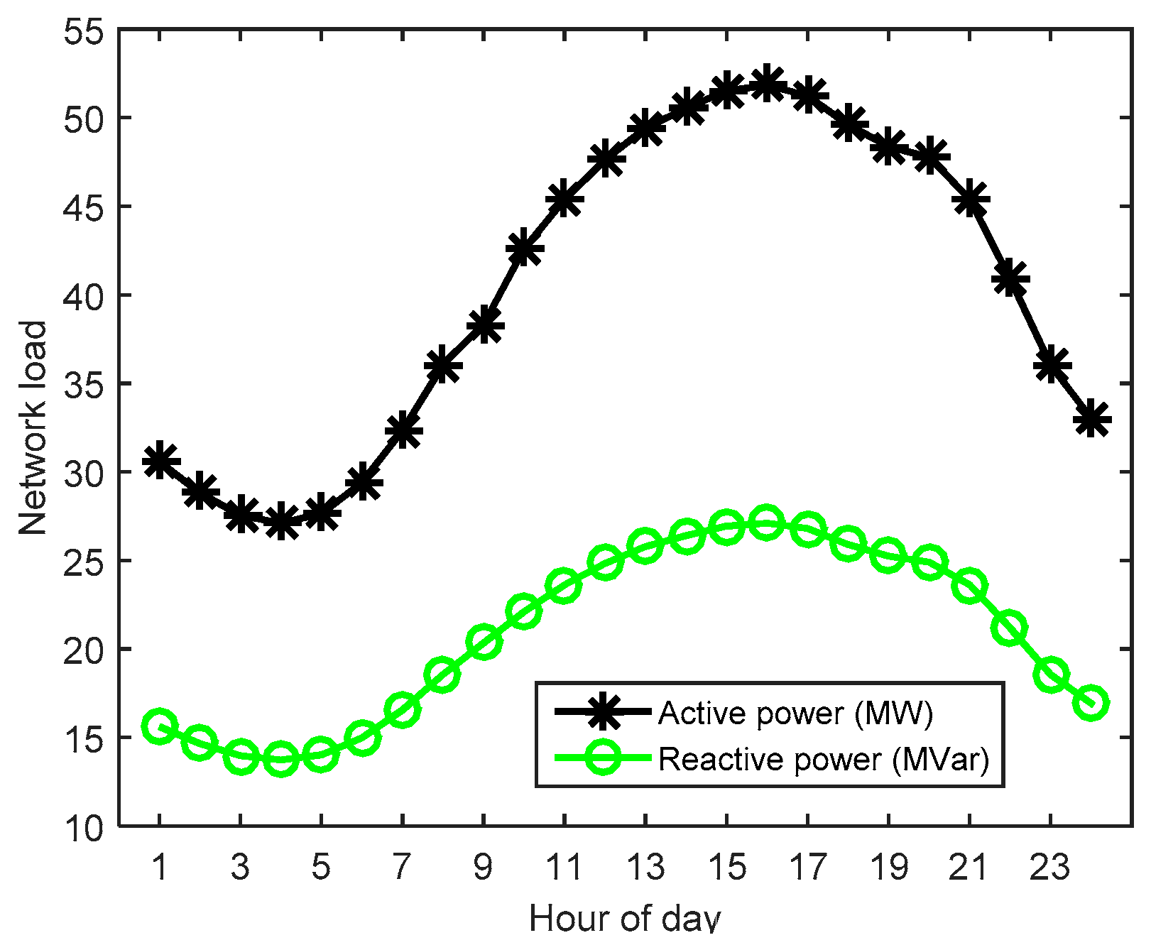
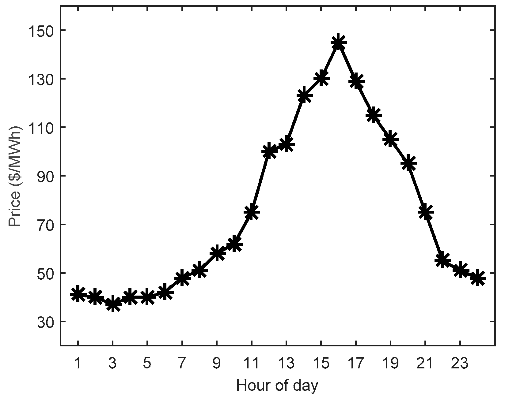
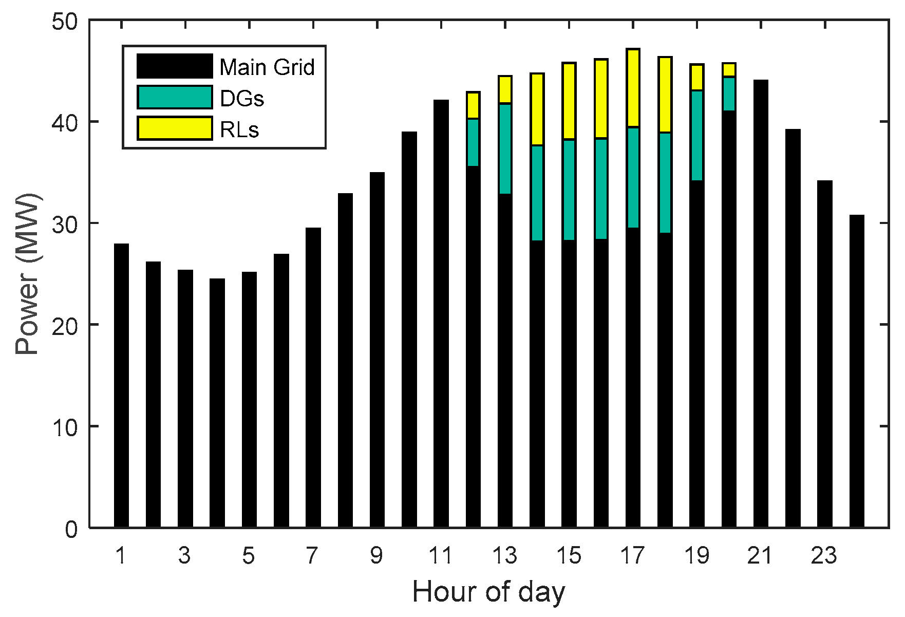
In the evolution process, if one dimension of an individual X i = [ x 1 , x 2 , x D ] exceeds its corresponding feasible region [ x min , x max ] , it is generally reset to the boundary, namely x i = x max or x i = x min . However, many individuals that gather around the boundary are harmful for the algorithm convergence; thus, a boundary handing method is presented.
If x i > x max :
x i = { x max h × rand ( 0 , 1 ) × x max x max 0 x max + h × rand ( 0 , 1 ) × x max x max < 0
If x i < x min :
x i = { x min + h × rand ( 0 , 1 ) × x min x min 0 x min h × rand ( 0 , 1 ) × x min x min < 0
where h is a user-specified constant. Through the method, the individuals which beyond the limits are distributed in a feasible region instead of on the boundary, so it increases the population diversity to a certain extent and accelerates the algorithm convergence.

5. Case Studies

This section is devoted to explore the efficiency of the proposed day-ahead optimal scheduling framework through the modified IEEE 33-bus distribution system [21,22]. Figure 1 shows the single line diagram of the 33-bus radial distribution system. In the network, three diesel-based DGs are supplemented at buses 7, 13, and 25 whose characteristics are provided in Table 1. Additionally, the system includes two 2 MW DFIG-based WTs and two 2 MW VSI-based PVs at buses 14, 17, 2, 4 and 31, respectively. The loads at buses 24 and 30 are considered as RLs with constant PF which can be curtailed up to 10 percent of their actual demand. The contract price for 1 MW curtailed by RLs is determined as $115/MW. Bus 1 is the only substation connected to the wholesale market.
In the test cases, the main assumption is that the forecast of WT power, PV power, and load profiles are fairly accurate; thus, the prediction errors are considered negligible. Figure 2 shows the network day-ahead predicted total load and the scaled wholesale market prices are demonstrated in Figure 3. Supposing that two WTs and two PVs are, respectively, faced with similar geographical conditions, the power generations by WTs and PVs are shown in Figure 4. Table 2 lists the maintenance cost of DERs. Emission quantity and emission cost for thermal power and DGs power are provided in Table 3 [23,24]. The cost coefficient of network loss is considered to be equal to the electricity price.
In order to examine the efficiency of the proposed scheduling framework, two scenarios are devised here. First, DMS determines the optimal solution of the available active elements including the reactive power support capabilities of WTs and PVs. Second, WTs and PVs are evoked only to output active power without the reactive power support capabilities. In the simulations, the proposed algorithm (MDE) is adopted to solve the problem. In the algorithm, the population size N and maximum number of iterations Gmax are, respectively, set to 100 and 200 for all cases; when initialized, the scaling factor ( F i , 0 ) and crossover rate ( CR i , 0 ) are randomly generated within the given range (0,1].

5.1. Considering the Reactive Power Support Capabilities of WTs and PVs

The proposed scheduling model seek the optimal scheduling of active elements by minimizing the economic costs of ADN. In order to assess the effects of different cost functions on the scheduling results, four cases are tested.
  • Case 1: the operation cost is considered as the objective function;
  • Case 2: the emission cost is considered as the objective function;
  • Case 3: the network loss cost is considered as the objective function; and
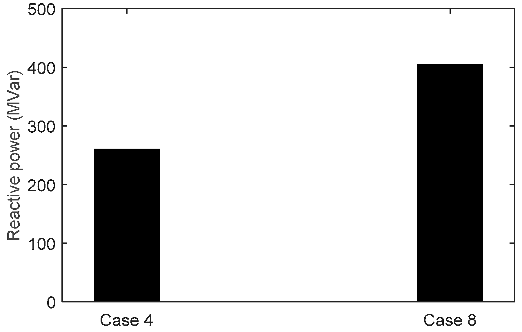
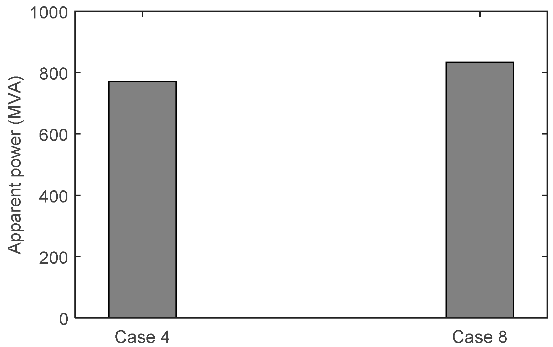
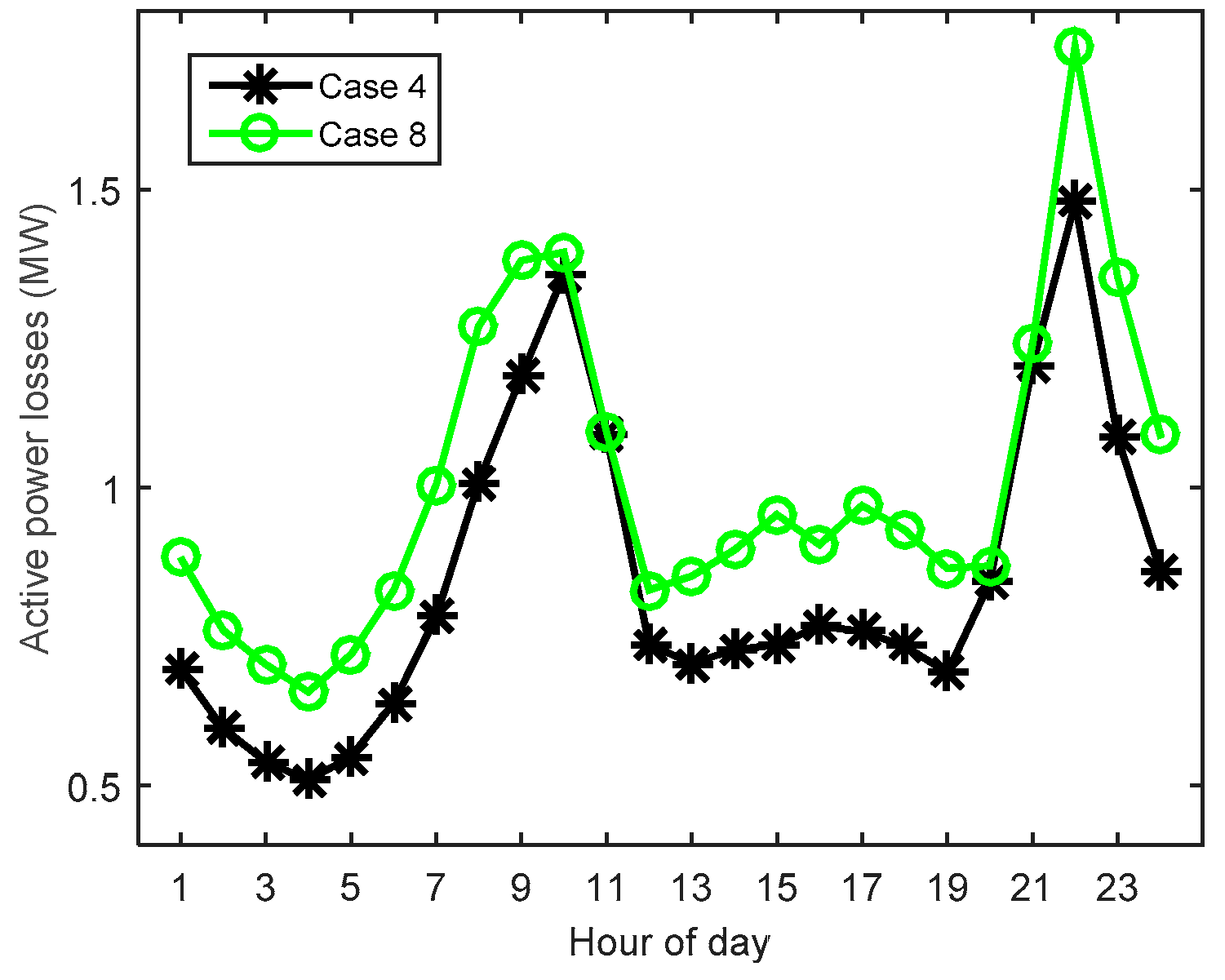
  • Case 4: the composite cost including operation cost, emission cost, and network loss cost is considered as the objective function.
The energy resource scheduling for Cases 1–4 are demonstrated in Figure 5, Figure 6, Figure 7 and Figure 8. It can be seen from Figure 5 that, in Case 1, DGs and RLs are made on during peak hours 12–20 to meet the network load when their costs are lower than the market electricity price; during hours 1–11 and 21–24, the network load demand is less and the market electricity price is low, DGs and RLs are switched off. The distribution purchases all of its requirements from the wholesale market. As the emission cost of DGs’ power are less than the purchased power (thermal power) and RLs’ participation can decrease the load demand to reduce the emissions; meanwhile, the dispatches of DGs and RLs can also reduce the network loss with the alteration of the network power flow distribution; hence, Figure 6 and Figure 7 shows that DGs and RLs are switched on during all the hours in Cases 2–3. Case 4 takes the composite cost as objective function and notable changes can be observed from Figure 8. Compared with Case 1, RLs and DGs are, respectively, scheduled from hours 10 and 11; their dispatch time continues to hour 21. In these hours, due to the participation of DERs, the operation cost may increase, but the emission and active power loss will drop largely. Thus, the composite cost would be a minimum. Furthermore, in comparison to Case 1, the RLs’ participation in Case 4 are significantly more.
Table 4 depicts the optimal hourly operation costs, emission costs, and active power loss costs of the distribution network for Cases 1–4. As it is seen, the total operation cost in Case 1 ($73,229.59), emission cost in Case 2 ($12,879.09), and network loss cost in Case 3 ($983.94) are, respectively, minimum for the individual cost in Cases 1–4. The corresponding individual costs in Case 4 are all more than them; but the composite cost in Case 4 is the minimum in Cases 1–4, which is $89,415.89. It can be observed that the total operation cost in Case 4 is $214.64 higher than Case 1; but with respect to the emission cost and network loss cost, Case 4 is, respectively, $654.26 and $297.03 lower than Case 1. Thus, the composite cost for Case 4 is $736.65 lower than Case 1. Compared with Cases 2 and 3, due to the dispatches of DERs in off-peak hours for Cases 2–3, namely hours 1–11 and 21–24, the operation costs are too high; hence, the composite cost for Case 4 is, respectively, $7,542.85 and $7,569.25 lower than Cases 2 and 3.
Cases 1–4 demonstrate the superiority and effectiveness of the proposed scheduling framework. The presented algorithm MDE have solved the nonlinear optimization problem effectively. In order to further illustrate the advantage of MDE, Particle Swarm Optimization (PSO) [25,26], DE [16], and MDE are used, respectively, to solve Case 4 ten times. In PSO and DE, the population size and maximum number of iterations are all set to 100 and 200. The acceleration constants c 1 ,   c 2 are set to 2; the maximum and minimum inertia weight factor ω are set, respectively, to 0.9 and 0.4 in PSO. In DE, the scaling factor (F) and crossover rate (CR) are set, respectively, to 0.2 and 0.6. The statistical result is shown in Table 5. It can be seen that MDE obtains the minimum values of composite cost and its standard deviation. Thus, MDE has the better performance on optimizing capacity and algorithm robustness.

5.2. Non-Considering The Reactive Power Support Capabilities of WTs and PVs

To assess the effect of reactive power support capabilities of WTs and PVs on the scheduling result, Cases 5–8 are added. They are similar to Cases 1–4, but in the Cases 5–8, the WTs and PVs are evoked only to output active power without the reactive power support capabilities.
  • Case 5: the operation cost is considered as the objective function where WTs and PVs are evoked only to output active power.
  • Case 6: the emission cost is considered as the objective function where WTs and PVs are evoked only to output active power.
  • Case 7: the network loss cost is considered as the objective function where WTs and PVs are evoked only to output active power.
  • Case 8: the composite cost is considered as the objective function where WTs and PVs are evoked only to output active power.
Figure 9, Figure 10, Figure 11 and Figure 12 show the energy resource scheduling for Cases 5–8. It can been seen that in Case 5, DGs and RLs are, respectively, switched on during peak hours 12–20 and 11–20; in Cases 6 and 7, DGs and RLs are switched on during all hours, as well as in Cases 2–3; in Case 8, DGs and RLs are, respectively, scheduled during hours 11–21 and 9–22. The optimal economic costs associated with Cases 5–8 are depicted in Table 6. As it is seen, the total composite cost in Case 8 ($90,400.01) is also the minimum compared with Cases 5–7. Thus, in Cases 5–8, which do not consider the reactive power support capabilities of WTs and PVs, the proposed composite cost objective function is also effective and achieves the minimum composite economic cost of the distribution network. Comparing Table 4 and Table 6, four comparisons between Cases 1 and 5, Cases 2 and 6, Cases 3 and 7, and Cases 4 and 8 are developed, it can be found that considering the reactive power support capabilities of WTs and PVs, the total daily composite cost in Cases 1–4 are $90,152.54, $96,958.74, $96,985.14 and $89,415.89 which are, respectively, $934.77, $833.78, $866.66 and $984.12 lower than Cases 5–8. Therefore, the conclusion can be drawn that implementation of the reactive power support capabilities of WTs and PVs can effectively decrease the economic cost of the network.
To further illustrate the effect of reactive power support capabilities of WTs and PVs, Case 4 and Case 8 are used for analysis. In Cases 4 and 8, the proposed composite cost is both considered as the objective function. Figure 13 explores the imported total reactive power from the main grid in the optimal day-ahead scheduling framework. It can be observed that because of the reactive power support capabilities of WTs and PVs, the total reactive power injected from the main grid in Case 4 is much less than Case 8. Meanwhile, as Figure 14 shows, the total apparent power injected from the main grid in Case 4 is also less than Case 8. Additionally, the network loss is usually concerned when the reactive power of distribution is optimally dispatched. Figure 15 depicts the hourly network losses for Cases 4 and 8. In Case 8, the main reactive power source is the wholesale market, but in Case 4, WTs and PVs integrated into ADN are also used as reactive power sources to accommodate the network demand. Thus, the reactive power regulation means Case 4 is more flexible. Accordingly, as it is seen, the total network losses for Case 4 are evidently less than Case 8.

6. Conclusions

This paper presented an intelligent day-ahead scheduling program for a smart distribution grid. In the program, a composite economic cost objective function is established which involves the operation cost, emission cost, and network loss cost; additionally, the reactive power support capabilities of WTs and PVs are considered in the optimal energy resources scheduling. Through simulation studies, it can be observed that considering the composite cost of ADN, the total daily operation cost increases, but the emission cost and network loss cost decline more; thus, the total daily composite cost would be the minimum. Meanwhile, implementation of the reactive power support capabilities of WTs and PVs has reduced the imported reactive power from external grid and improved the economic benefit of ADN by decreasing the total daily composite cost. The total network loss of the system is decreased as well. Results certify the validity of the proposed methodology in the optimal scheduling of a smart distribution grid.

Acknowledgments

This work was supported by the research funding of School of Electrical Engineering, Wuhan University. This sponsorship is gratefully acknowledged.

Author Contributions

Rongxiang Yuan and Timing Li proposed the concrete ideas of the work; Timing Li and Xiangtian Deng conceived and designed the experiments; Jun Ye performed the experiments and analyzed the data; Timing Li wrote the paper.

Conflicts of Interest

The authors declare no conflict of interest.

References

  1. Ramachandran, B.; Srivastava, S.K.; Edrington, C.S.; Cartes, D.A. An intelligent auction scheme for smart grid market using a hybrid immune algorithm. IEEE Trans. Ind. Electron. 2011, 58, 4603–4612. [Google Scholar] [CrossRef]
  2. D’Adamo, C.; Jupe, S.; Abbey, C. Global survey on planning and operation of active distribution networks-Update of CIGRE C6.11 working group activities. In Proceedings of the 20th International Conference and Exhibition on Electricity Distribution (CIRED 2009), Prague, Czech Republic, 8–11 June 2009.
  3. Algarni, A.A.S.; Bhattacharya, K. Disco operation considering DG units and their goodness factors. IEEE Trans. Power Syst. 2009, 24, 1831–1840. [Google Scholar] [CrossRef]
  4. Pilo, F.; Pisano, G.; Soma, G.G. Optimal coordination of energy resources with a two-stage online active management. IEEE Trans. Ind. Electron. 2011, 58, 4526–4537. [Google Scholar] [CrossRef]
  5. Silva, M.; Morais, H.; Vale, Z. An integrated approach for distributed energy resource short-term scheduling in smart grids considering realistic power system simulation. Energy Convers. Manag. 2012, 64, 273–288. [Google Scholar] [CrossRef]
  6. Doostizadeh, M.; Ghasemi, H. Day-ahead scheduling of an active distribution network considering energy and reserve markets. Int. Trans. Elect. Energy Syst. 2013, 23, 930–945. [Google Scholar] [CrossRef]
  7. Sousa, T.; Morais, H.; Vale, Z.; Castro, R. A multi-objective optimization of the active and reactive resource scheduling at a distribution level in a smart grid context. Energy 2015, 85, 236–250. [Google Scholar] [CrossRef]
  8. Vahidinasab, V.; Jadid, S. Joint economic and emission dispatch in energy markets: A multiobjective mathematical programming approach. Energy 2010, 35, 1497–1504. [Google Scholar] [CrossRef]
  9. Engelhardt, S.; Erlich, I.; Feltes, C.; Kretschmann, J.; Shewarega, F. Reactive power capability of wind turbines based on doubly fed induction generators. IEEE Trans. Energy Convers. 2011, 26, 364–372. [Google Scholar] [CrossRef]
  10. Meegahapola, L.; Durairaj, S.; Flynn, D.; Fox, B. Coordinated utilisation of wind farm reactive power capability for system loss optimization. Eur. Trans. Electr. Power 2011, 21, 40–51. [Google Scholar] [CrossRef]
  11. Zou, K.; Agalgaonkar, A.P.; Muttaqi, K.M.; Perera, S. Distribution system planning with incorporating DG reactive capability and system uncertainties. IEEE Trans. Sustain. Energy 2012, 3, 112–123. [Google Scholar] [CrossRef]
  12. Rueda-Medina, A.C.; Padilha-Feltrin, A. Distributed generators as providers of reactive power support—A market approach. IEEE Trans. Power Syst. 2013, 28, 490–502. [Google Scholar] [CrossRef]
  13. El-Shimy, M. Modeling and analysis of reactive power in grid-connected onshore and offshore DFIG-based wind farms. Wind Energy 2014, 17, 279–295. [Google Scholar] [CrossRef]
  14. Delfino, F.; Denegri, G.B.; Invernizzi, M.; Procopio, R.; Ronda, G. A P-Q capability chart approach to characterize grid connect PV-units. In Proceedings of the Integration of Wide-Scale Renewable Resources into the Power Delivery System, 2009 CIGRE/IEEE PES Joint Symposium, Calgary, AB, Canada, 29–31 July 2009.
  15. Lof, P.A.; Andersson, G.; Hill, D.J. Voltage-dependent reactive power limits for voltage stability studies. IEEE Trans. Power Syst. 1995, 10, 220–228. [Google Scholar] [CrossRef]
  16. Storn, R.; Price, K. Differential evolution—A simple and efficient heuristic for global optimization over continuous spaces. J. Glob. Optim. 1997, 11, 341–359. [Google Scholar] [CrossRef]
  17. Noman, N.; Iba, H. Differential evolution for economic load dispatch problems. Electr. Power Syst. Res. 2008, 78, 1322–1331. [Google Scholar] [CrossRef]
  18. Abou El Ela, A.A.; Abido, M.A.; Spea, S.R. Differential evolution algorithm for optimal reactive power dispatch. Electr. Power Syst. Res. 2011, 81, 458–464. [Google Scholar] [CrossRef]
  19. Abaci, K.; Yamacli, V. Differential search algorithm for solving multi-objective optimal power flow problem. Int. J. Electr. Power Energy Syst. 2016, 79, 1–10. [Google Scholar] [CrossRef]
  20. Duwuru, N.; Swarup, K.S. A hybrid interior point assisted differential evolution algorithm for economic dispatch. IEEE Trans. Power Syst. 2011, 26, 541–549. [Google Scholar]
  21. Wong, S.; Bhattacharya, K.; Fuller, J.D. Electric power distribution system design and planning in a deregulated environment. IET Gener. Transm. Distrib. 2009, 3, 1061–1078. [Google Scholar] [CrossRef]
  22. Sousa, T.; Morais, H.; Vale, Z.; Faria, P.; Soares, J. Intelligent energy resource management considering vehicle-to-grid: A simulated annealing approach. IEEE Trans. Smart Grid 2012, 3, 535–542. [Google Scholar] [CrossRef]
  23. Ding, M.; Zhang, Y.Y.; Mao, M.Q.; Yang, W.; Liu, X.P. Steady model and operation optimization for microgrids under centralized control. Automat. Electron. Power Sys. 2009, 33, 78–82. [Google Scholar]
  24. Deng, W.; Li, X.R.; Liu, Z.Y.; Yan, Y.L.; Li, J.X.; Ma, Y.H. Comprehensive optimal allocation of intermittent distributed generation considering reactive power compensation. CSEE J. Power Energy Syst. 2012, 32, 80–88. [Google Scholar]
  25. Hassan, M.A.; Abido, M.A. Optimal design of microgrids in autonomous and grid-connected modes using particle swarm optimization. IEEE Trans. Power Electron. 2011, 26, 755–769. [Google Scholar] [CrossRef]
  26. Singh, S.P.; Rao, A.R. Optimal allocation of capacitors in distribution systems using particle swarm optimization. Int. J. Electr. Power Energy Syst. 2012, 43, 1267–1275. [Google Scholar] [CrossRef]
Figure 1. Single line diagram of the IEEE-33 bus test system.
Energies 09 00311 g001
Figure 2. Day-ahead forecasting load profile.
Energies 09 00311 g002
Figure 3. Day-ahead wholesale market prices.
Energies 09 00311 g003
Figure 4. Forecasted power output of WTs and PVs.
Energies 09 00311 g004
Figure 5. Energy resources scheduling results for Case 1.
Energies 09 00311 g005
Figure 6. Energy resources scheduling results for Case 2.
Energies 09 00311 g006
Figure 7. Energy resources scheduling result for Case 3.
Energies 09 00311 g007
Figure 8. Energy resources scheduling result for Case 4.
Energies 09 00311 g008
Figure 9. Energy resources scheduling results for Case 5.
Energies 09 00311 g009
Figure 10. Energy resources scheduling results for Case 6.
Energies 09 00311 g010
Figure 11. Energy resources scheduling results for Case 7.
Energies 09 00311 g011
Figure 12. Energy resources scheduling results for Case 8.
Energies 09 00311 g012
Figure 13. Imported total reactive power from the main grid in Cases 4 and 8.
Energies 09 00311 g013
Figure 14. Imported total apparent power from main grid in Cases 4 and 8.
Energies 09 00311 g014
Figure 15. Active power losses of the network in Cases 4 and 8.
Energies 09 00311 g015
Table 1. DGs’ characteristics and cost data.
UnitFuel Cost Function CoefficientsTechnical Constraints
ai $/MW2bi $/MWci $SUDG,i $SDDG,i $ P DG , i min MW P DG , i max MWRRi MW/min
DG10.0045792715100.7530.025
DG20.0045872515100.7530.025
DG30.003581261510140.03
Table 2. DERs’ maintenance cost.
DG1 $/MWDG2 $/MWDG3 $/MWWT1 & 2 $/MWPV1 & 2 $/MW
Maintenance cost coefficients7896.83
Table 3. Emission characteristics and cost data.
Emission SpeciesEmission Rate (Kg/MW)Emission Fees $/Kg
Thermal PowerDGs Power
CO28896490.019
SO21.80.2060.236
NOx1.69.890.472
Table 4. Hourly costs in Cases 1–4.
HourCase 1Case 2Case 3Case 4
A ($)B ($)C ($)A ($)B ($)C ($)A ($)B ($)C ($)A ($)B ($)C ($)
11,261.31502.5627.321,806.09401.2310.141,806.23401.499.891,261.31502.5627.32
21,169.68473.0222.601,926.31362.655.461,926.41363.505.161,169.68473.0222.60
31,065.23457.1819.341,873.82353.724.631,873.82353.824.611,065.23457.1819.34
41,106.57442.8921.231,863.17340.134.401,862.73340.784.281,106.57442.8921.23
51,111.34454.6422.271,914.90358.504.921,914.73359.214.631,111.34454.6422.27
61,238.52486.1327.132,020.38382.166.152,020.17382.516.021,238.52486.1327.13
71,526.11531.7737.232,245.65420.578.672,245.51420.648.701,526.11531.7637.23
81,788.20594.9151.052,489.30470.7112.582,489.87471.4612.541,788.20594.9151.05
92,135.39631.6069.722,733.23494.6418.702,733.10497.2518.052,135.39631.6069.72
102,520.88703.8294.313,075.75553.1926.723,073.45554.6326.122,542.32655.3266.20
113,259.46753.15136.363,580.62600.8743.223,580.08602.0842.663,312.37660.0874.87
124,381.75712.27100.534,358.70623.6264.364,357.32623.9462.134,388.53627.3166.71
134,592.62749.2187.944,626.23653.7271.874,626.14654.3071.114,590.40652.4571.34
145,238.74660.3088.525,283.81658.1788.145,283.17667.4586.085,283.74663.4389.86
155,569.56678.7598.035,571.54675.3099.415,570.10686.7396.045,569.83677.8896.33
166,027.52680.43115.496,031.16679.52111.256,030.55688.53110.436,027.52679.62111.87
175,661.43703.67101.325,668.57694.87101.545,668.80704.8299.685,661.51694.9098.73
185,191.29691.4186.015,200.92689.0286.795,198.72691.5884.055,191.30689.1484.60
194,800.46787.10107.534,795.81670.3674.604,796.56670.6274.464,796.37670.7174.68
204,471.30790.63131.684,489.46668.0167.224,487.32671.0664.924,510.21678.8380.25
213,409.43791.02146.623,738.31632.7844.913,737.65635.5343.253,465.17697.5781.64
222,265.71703.5583.412,926.10566.8124.562,926.31567.5124.012,265.52703.8283.63
231,850.37613.5356.352,543.82491.5315.082,543.49491.8814.901,850.37613.5356.36
241,586.72554.9342.492,310.37437.0110.312,310.36437.2910.221,586.72554.9342.49
Total7,3229.591,5148.471,774.488,3074.021,2879.091,005.638,3062.5912,938.61983.9473,444.231,4494.211,477.45
S90,152.5496,958.7496,985.1489,415.89
A, B and C respectively denote the operation cost, emission cost and network loss cost of the distribution; S denotes composite cost (S = A + B + C).
Table 5. Statistical result of different algorithms.
AlgorithmAverage Operation Cost ($)Average Emission Cost ($)Average Network Loss Cost ($)Average Composite Cost ($)Composite Cost Standard Deviation
PSO7,3671.871,4539.391,480.8389,692.0941.22
DE7,3657.021,4535.071,481.6489,673.7339.67
MDE7,3452.511,4498.251,479.3889,430.1411.60
Table 6. Economic costs associated with Cases 5–8.
Total Operation Cost ($)Total Emission Cost ($)Total Network Loss Cost ($)Total Composite Cost ($)
Case 573,637.4115,283.042,166.8691,087.31
Case 683,462.2713,021.111,309.1497,792.52
Case 783,446.5813,118.721,286.5097,851.80
Case 873,983.5214,617.261,799.2390,400.01

