Abstract
For over three decades the “Pendulor” wave energy device has had a significant influence in this field, triggering several research endeavours. It includes a top-hinged flap propelled by the standing waves produced in a caisson with a back wall on the leeward side. However, one of the main disadvantages which impedes its progress is the enormous expense involved in the construction of the custom made typical caisson structure, about a little more than one-quarter of the wave length. In this study, the influence of such design parameters on the performance of the device is investigated, via numerical modelling for a device arranged in an array configuration, for irregular waves. The potential wave theory is applied to derive the frequency-dependent hydrodynamic parameters by making a distinction in the fluid domain into a separate sea side and lee side. The Cummins equation was utilised for the development of the time domain equation of motion while the transfer function estimation methods were used to solve the convolution integrals. Finally, the device was tested numerically for irregular wave conditions for a 50 kW class unit. It was observed that in irregular wave operating conditions, the caisson chamber length could be reduced by 40% of the value estimated for the regular waves. Besides, the device demonstrated around 80% capture efficiency for irregular waves thus allowing provision for avoiding the employment of any active control.
1. Introduction
To date, no particular distinct method exists for harnessing wave energy, although several types of devices have been developed using a gamut of approaches. The Pendulor device, among the class of terminators is one of the pioneers in this field. This device works in a manner quite opposite to that of the top-hinged flap type wave maker (Figure 1). Although the Muroran Institute of Technology (Japan) produced the Pendulor device as a result of the work done in the early 1980s [1], several efforts continue to be made to improve it [2]. A good percentage of these studies were focused mainly only on experimental verification, and most reports recorded that a conversion efficiency of 40%–60% was possible by the systems for sea conditions prevailing in the Muroran bay at peak wave considitons [3,4,5]. The experimental laboratory results of these Pendulor devices indicated that the primary energy conversion efficiency can reach up to 82% for regular waves [6]. Following this, several trials have been conducted at sea using these Pendulor type devices in Japan, at two places in Hokkaido [7]. All the studies reported good device performance for conversion efficiency. More recent studies have paid greater attention to improve the secondary power transmission unit, like the rotary vane pump [5]. In Japan and Korea recent research work studied a floating version of the device as an offshore version, in which the caisson is integrated into a stabilised floater [8]. Another device closely resembling the Pendulor is the early version of Oscillating Surge Wave Converter (OSWC). That is different from Pendulor in concept, as it uses an oscillating water column rather than a straight chamber on the lee side [9]. With respect to the original concept of the Pendulor, the flap fucntions at the node point of the standing waves produced in a straight caisson where the maximum wave surging effect is felt. Thus, the caisson significantly affects the the device performance. Several studies are currently being conducted to identify superior caisson configurations to enhance the device performance and optimise the caisson size at the same time [10].
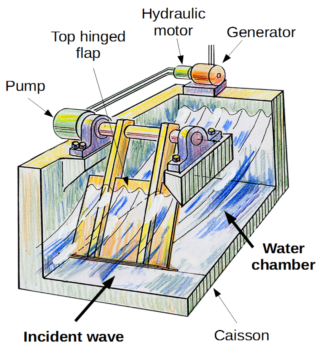
Figure 1.
Concept of the “Pendulor” device [7].
The Pendulor wave energy devices (mostly employed as pilot plants) were initially based on the approximations of the regular wave model. These devices had caissons costing about one-third or more of the total construction expense, rendering it one of the major obstacles for further development [11]. Pendulor devices used as an integral part of a double purpose breakwater system could become a possibility to overcome this disadvantague. This type of breakwater system will have a larger breadth than the regular one because of the effect of the caisson length which extends to the sea side. According to regular wave approximations this length should equal one-quarter of the significant wave length to achieve maximum efficiency [7]. Thus, for seas with long waves, the chamber length becomes more than 25 m, resulting in exorbitant construction expenditure and other related issues. However, all the sea trials were performed by maintaining the chamber length to around the generally accepted parameters, of one-quarter of the wave length predicted. Furthermore, from the practical viewpoint, flap repositioning is not that easy during real sea trials to explore its effect on device performance. To surmount these problems it appears to be cost effective to develop a numerical model for irregular wave conditions so that the system characteristics can be studied under realistic operating conditions. Models of this type will also prove central for optimising several other geometrical and inertial parameters of the device, structural loading control [12], and improving device control strategies related to irregular wave conditions. Therefore, a numerical model has been developed for the Pendulor wave energy device arranged in an array configuration for regular and irregular waves. The model also is used to discuss the probable optimisation of the device parameters.
The potential theory for the Pendulor device is precented by employing a new and succinct approach quite distinct from the original version [7]. This was done by integrating the recognised wave maker theories (refer to the annex in the Appendix A) with the traditional potential theory. In this case, the flap motion was replicated by the collective movement of a flap hinged at the bottom and a piston oscillating horizontally. The possible functions related to the two distinct cases were combined together to achieve the corresponding total potential function of the top-hinged flap motion and thus making it possible to identify the frequency-dependent hydrodynamic parameters. Next, to identify the features of the device under regular wave conditions, a frequency domain analysis was performed. To facilitate the analysis of the system during irregular wave conditions, a time domain model was also developed on the basis of the Cummins [13] equation which uses the convolution integral. The impulse response functions based on the frequency domain models were found by applying the approximation methods to reduce computational time [14,15,16,17]. The time domain model is shown to agree with the corresponding frequency domain theoretical data. The analysis of the motion response and corresponding power conversion capability of the device conducted based on these models are discussed subsequently for the regular and irregular wave conditions related to the southern coastal wave climate in Sri Lanka, based on the feasibility studies of Watabe et al. [11] and Amarasekara et al. [18].
2. Formulation of the Problem
2.1. Governing Equation
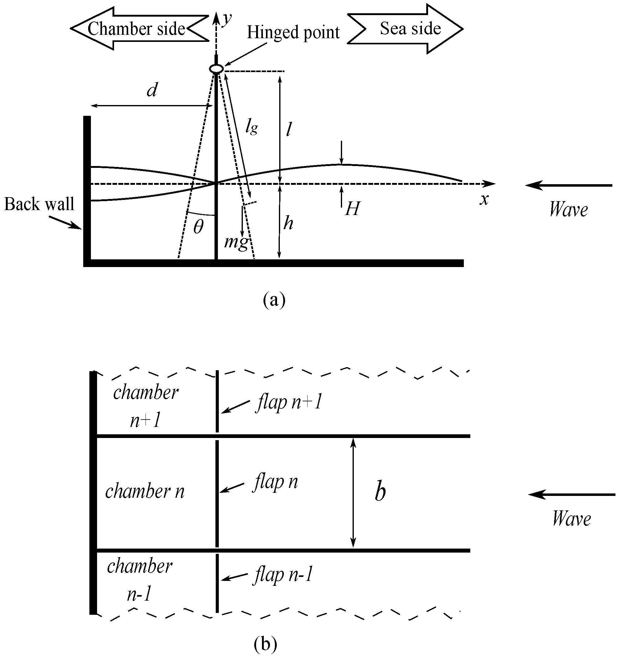
Figure 2 is the schematic representation of the “Pendulor” device in a straight caisson. Supposing the flap is completely extended to the bottom and tightly fitted to the chamber width, the flow across the flap is assumed to be negligible for the smaller angles of oscillations. Hence, the fluid domain is assumed to be distinguishable into individual regions by the flap as the sea side (side s) and lee side (side c, which hereafter is referred to as chamber side). The fluid flow is considered inviscid, incompressible and irrotational. A Cartesian coordinated system is employed here in which the plane is occupied by the undisturbed water surface and the x-axis is directed orthogonal to the flap. The y-axis (+ve) is directed vertically upwards and the z-axis can be ignored for a purely two-dimensional problem (as the flaps are arranged in an array of a breakwater). The angle of the flap oscillation is (+ve counter-clockwise) and t indicates the time. The flap is hinged at . The bottom of the caisson and side walls are occupied plane and planes, respectively. The caisson back wall is at plane.

Figure 2.
Schematic representation of the Pendulor device in a breakwater ((a) side elevation; (b) plan elevation).
When Newton’s law of motion is applied to the flap, the single degree of freedom equation of motion can be simply expressed as:
in which is the moment of inertia of the flap about the hinged point, is the restoring moments applied by the flap mass, is the hydrodynamic and hydrostatic moments acting on the flap, is the external mechanical torque on the flap related to the power take off system and is the drag moment exerted on the flap. Assuming that the angle of oscillation of the flap is small and has no flow condition present across the flap, the drag moment can be ignored. The hydrostatics and hydrodynamics moments can further be decomposed, where is the buoyancy moment (for a thin flap, ), is the radiation moment and is the excitation moment.
2.2. Governing Equation in Frequency Domain (Linear System)
For a harmonic wave of frequency ω, the radiation moment can be decomposed as follows:
where I is the frequency dependent added inertia, B is the frequency dependent radiation damping, and K is the hydrostatic restoring coefficient (spring constant). Assuming the Power take off (PTO) system is linear, it is best expressed as:
where N is the damping coefficient of PTO and is the restoring coefficient of PTO. As the flap oscillates in small angles, the restoring moment due to the inertia of the flap can be expressed as , where is the distance between the hinged point and the centre of gravity of the flap, m is the flap mass and g is the acceleration due to gravity. Therefore, the Equation (1) can now be expressed as:
Considering a harmonic wave of frequency ω, and . Where α is the phase difference. Therefore, the amplitude of flap oscillation can now be expressed as:
The non dimensional Capture factor is found by using Equations (A30), (A34) and (A36) (refer Appendix A) as:
Time averaged power of incoming wave of height H is:
where b is the width of the flap, ρ is the static density of water, is the given by the dispersion relationship where and h is the water depth.
shown in Equation (7) is achieved to 1 for the regular waves at resonance condition (Equation (9)) and impedance matching condition (Equation (10)).
During actual sea operations, the incoming wave frequencies are normally found to hover between 0.5 and 0.9 rad/s. To complement that requirement, most of the point absorbers and OWCs require negative values of PTO spring-stiffness . As the physical implementation itself of such systems is not easy, an alternative latching control was introduced by Budal and Falnes [20]. The Pendulor device, however, can be designed to match the incoming wave frequency by selecting the correct inertia of the flap and caisson profile. A few such features will be discussed in Section 3.
2.3. Governing Equation in Time Domain
Cummins [13] developed the linear time domain approach for floating marine structures in seas characterised by waves. Later, that theory was applied extensively to wave energy devices and associated applications [19,21,22,23]. For zero forward speed, by employing similar concepts, Equation (1) can be expressed in the form of Equation (11):
where is the impulse response function (memory function) and the convolution term .
As there are two hydrodynamic regions, it is fitting to decompose the impulse response in Equation (11) into two segments, one for the sea side and the other for the chamber side . Therefore, the governing equation is now expressed as:
The methods of attaining the convolution integral in terms of Equation (12) (corresponding radiation moments) will be discussed in Section 2.3.1 and Section 2.3.2.
2.3.1. Radiation Moment Function in Sea Side
The frequency-based hydrodynamic parameters obtained by the potential theories (discussed in the Appendix A) are used for the evaluation of the impulse response functions. As the hydrostatic restoring moment is lacking in the sea side due to continuous generation of waves by the flap motion, it is only the added inertia and the radiation damping that contribute to the radiation moments (refer to the Appendix A for more details).
The radiation moment acting on the sea side is , in which the subscript refers to the sea side. The radiation impedance of the sea side is expressed as , where and .
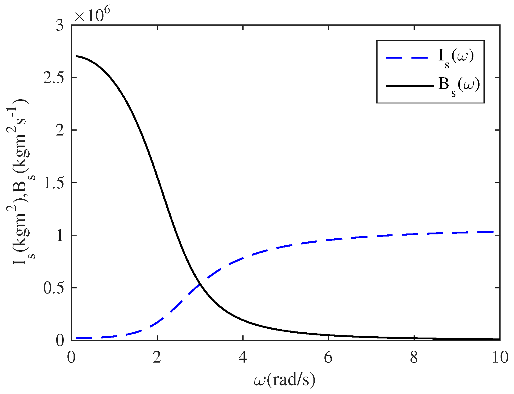
Hydrodynamics added inertia, radiation damping and excitation moments for sea side are expressed in Equations (13)–(15), respectively, for a harmonic wave of height H and frequency ω (refer to the Appendix A). The preliminary device parameters of the 50 kW unit based on the regular wave = 12 s and = 1 m are given in Table 1.

Table 1.
Preliminary device parameters of the 50 kW unit.
Figure 3 reveals the results of the added inertia and radiation damping with the frequency for a device with the parameters listed in Table 1.
where . Here, both and are even functions of ω as because standing waves need to be decayed away from the wave maker [24]. As evident in Figure 3, does not reach zero when as is anticipated in the 3D oscillating bodies. This is because of the 2D approximation made in the specific problem. Comparable results of this type have been reported in the works of Anami et al. [25], Lewandowski [26] (p. 233). Besides, Porter and Biggs [27] showed comparable results as can be seen for the 2D model of the bottom-hinged flap type wave energy device.
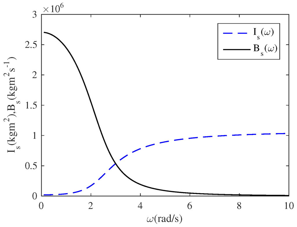
Figure 3.
Variation of added inertia (dotted line) and the radiation damping (solid line) with frequency .
The impulse response of the sea side can be calculated by employing either the added inertia or radiation damping data in the frequency domain [19]. Therefore, the radiation moments can be expressed as:
where
2.3.2. Radiation Moment Function in Chamber Side
In the chamber side, the added inertia and hydrostatic restoring moments alone constituted the hydrodynamic moments on the flap (refer appendix A). Damping was absent in the chamber side. All the energy contributed by the flap to the water mass returns once again back to the flap via the hydrostatic restoring action. The chamber side added inertia and hydrostatic restoring moment are expressed in Equations (20) and (21), respectively (see the same equations in the Appendix A as Equation (A27) and Equation (A26)). Figure 4 reveals the variation of the added inertia with frequency for the range 0 to 2 rad/s. The added inertia function reveals its asymptotic nature at the points ( is related to ω by dispersion relationship), where the anti-nodes of the standing waves in the chamber coincide with the flap. It is significant that the large negative or positive added inertias are found at those frequencies due to the production of great positive or negative pressures at the flap surface. These great negative pressures can induce a possible flow separation between the flap and water mass that generally affects the bodies with the surface piercing effect. Whereas, the hydrostatic restoring coefficient (given in Equation (21)) is dependent solely on the chamber geometry (refer to the Appendix A).
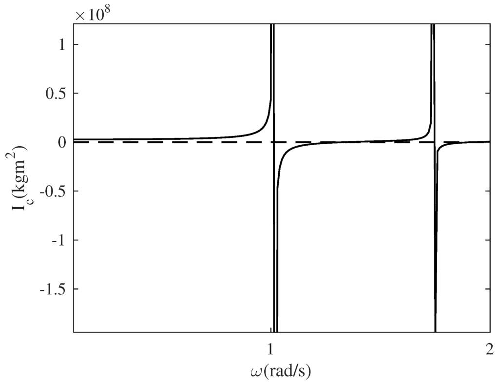
Figure 4.
Variation of added inertia () with wave frequency (ω).
The following equation shows the radiation moment acting on the chamber side using the convolution integral:
The radiation impedance is as follows:
where
2.4. System Identification
The direct numerical computation of the convolution integral in Equation (11) is a very time consuming operation. As the convolution term is a linear operation, an equivalent system can be achieved as a transfer function (TF) or state space model (SSM). In the literature, several related studies on the approximation of the convolution integral are available [14,15,16,17,22,28]. These are the well established methods, however, based on the type of the problem encountered minimal changes are anticipated. The methodologies included in this study have been highlighted for easy reader reference and to facilitate convenient replication of the results.
Here the TF model which can be approximated in two ways was employed. They are time domain identification (TDI) and frequency domain identification (FDI). Based on the features of the data, a suitable approximation technique was chosen after many trials using different methodologies. In this study, the approximation quality was observed considering the value, computed as follows.
where represents the approximated function and refers to the reference function, while gives the mean value reference function.
2.4.1. Sea Side System Identification
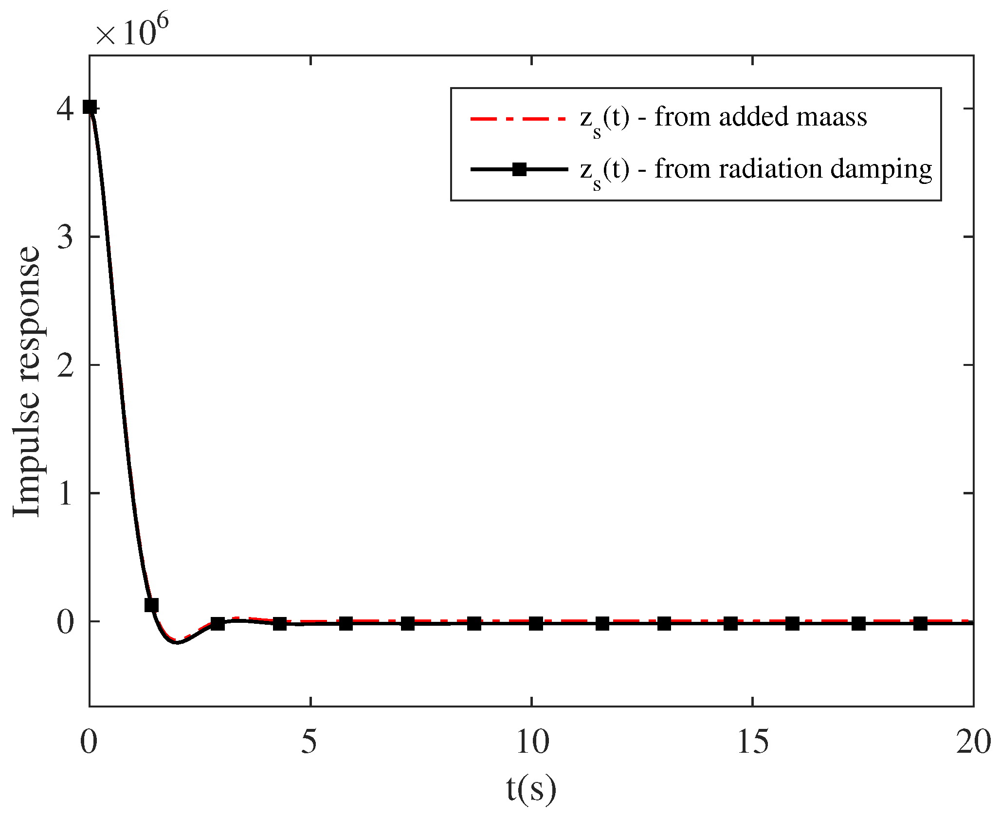
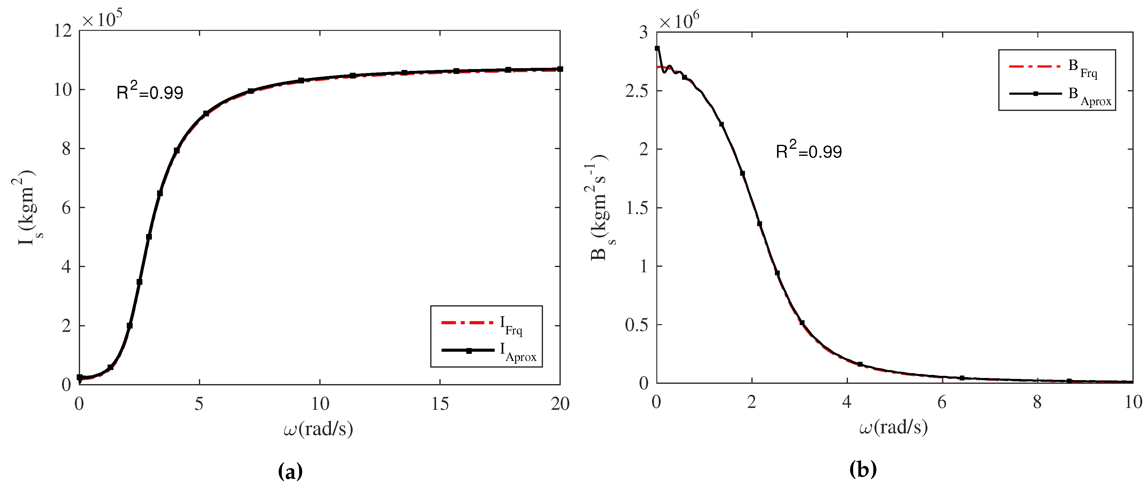
The TDI method is used to assess the sea side TF. The corresponding time domain impulse response function can be achieved by incoroporating the method of Ogilvie [29] as seen in Figure 5. The TF is thus approximated by utilising these data and the TDI method termed the least square method [15] based on the Matlab function “prony”, which converts the impulse response function to z-transformation. The discrete TF needs to be converted to the continuous time domain which can be done by using “d2c” function with the Tustin method in the Matlab control tool box [30]. The added inertia and radiation damping given by TF were thus identified. A comparison of these was done with the corresponding theoretical potential function as seen in Figure 6. Both functions are well fitted with accuracy.
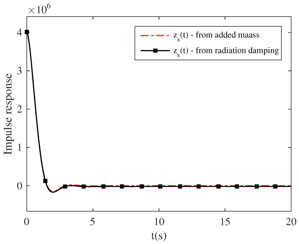
Figure 5.
Impulse response of added inertia and radiation damping.
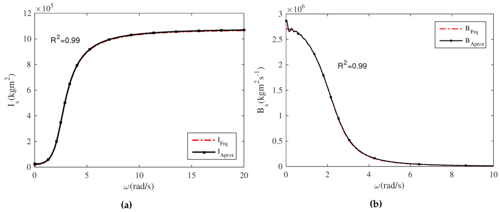
Figure 6.
(a) Added mass vs. ω; (b) Radiation damping vs. ω, indicates frequency domain data and transfer function approximation data (dashed red line; frequency domain data, solid line; transfer function approximation data).
2.4.2. Chamber Side System Identification
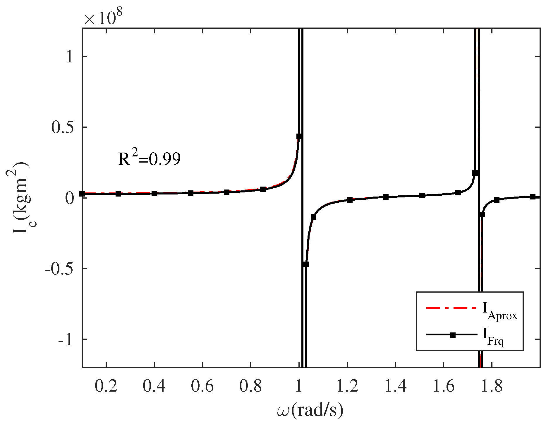
For the chamber side, trials conducted using the TDI methods produced poor matching results mostly because of the errors in the frequency response function caused by singularities in the added inertia function (as seen in Figure 4). A good alternative was the “tfest” command in Matlab [30] which was successful in approximating the TF directly without converting to the time domain. Therefore, the radiation moment function simply takes on the form of Equation (18) without modifying it with the limiting value of the term added inertia . In such cases, the frequency domain data were drawn from the area of interest in which a majority of the ocean waves were concentrated (0.1 to 2 rad/s). In Figure 7 the frequency domain data given by the approximated TF and frequency domain data of the potential functions for the added inertia were compared. Both are well fitted with accuracy.
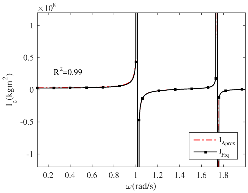
Figure 7.
Added inertia vs. ω of the chamber side for frequency domain and transfer function approximation (dashed red line; frequency domain data, solid line; transfer function approximation data).
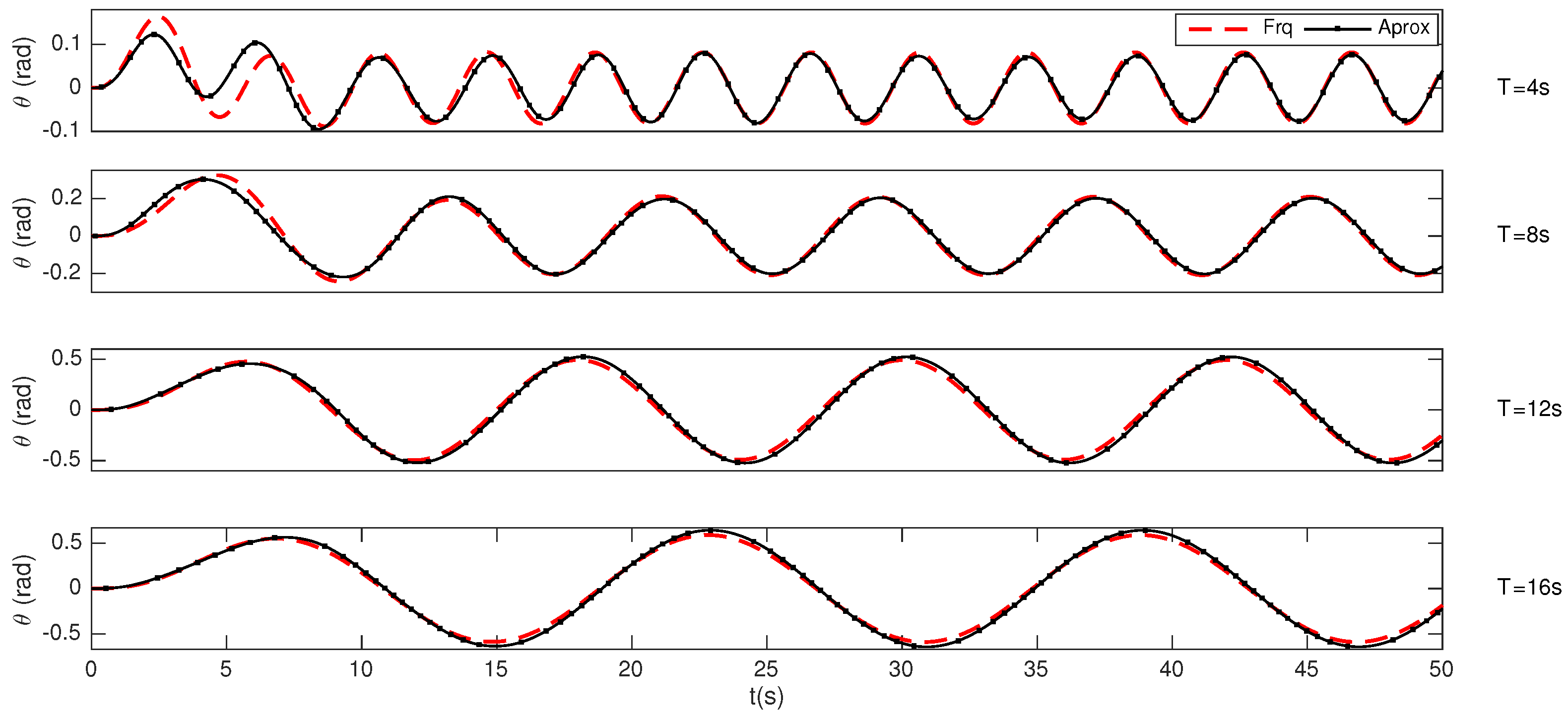
Combining the time domain models of the sea side and chamber side, the governing equation of the total system is expressed as given.
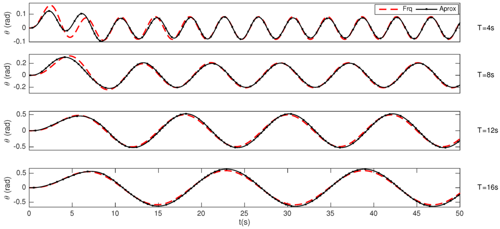
To verify the validity of the approximations, the time domain solutions of Equation (4) are compared with the corresponding solutions in Equation (25). Figure 8 lists the results of the amplitude of oscillations for different frequencies at no load condition () for 50 s duration. The dotted lines indicate the time domain results of Equation (4) whereas the solid lines imply the corresponding time domain solution of Equation (25). Both solutions are well fitted for the wider frequency range and thus the validity of the approximated time domain model is confirmed for further calculations.
3. Characteristics of the Plant
3.1. The Case of Regular Waves
In the case of regular waves This section discusses the device characteristics for simplified power take-off systems (PTO). Depending on the torque applied by the PTO system, the load torque could simply be modelled as linear damping torque (Equation (26)) or Coulomb type frictional torque (Equation (27)).
where, is the Coulomb damping torque. The features of the governing equations given above are dependent on the hydrodynamic/static parameters and the the type of the power take off system. The Linear damping gives 100% theoretical maximum efficiency (ignoring frictional losses) at the resonance conditions and impedance matching conditions as explained in Section 2.2. However, the linear damping PTO systems are not easy to put into practice and therefore most of the practical PTO systems can be modelled as Coulomb damping.
3.1.1. Linear Damping
The device dynamics can be obtained for linear damping in the frequency domain employing Equation (26). In order to utilise maximum power, it must fulfil the resonance condition , and impedance matching condition where is the resonance frequency. A dimensionless frequency is introduced as where . The total added inertia, radiation damping and hydrostatic restoring coefficient can be identified as and respectively. is ignored through the entire calculations assuming that the PTO system does not exist a restoring effect. The dimensionless frequency is plotted with the dimensionless chamber length as seen in Figure 9 in which the dimensionless chamber length is , dimensionless wave length is and λ is the incident wave length. Then indicates the flap resonance frequency, and it happens when attains the value , where the nodes of the standing wave are noted with reference to the back wall. Therefore, the placement of the flap at a node is crucial for the device performance (frequency matching) and the first node point is observed at one-quarter of the wave length from the back wall. For the device model in this study, the corresponding chamber length becomes to 18 m at the 12 s design wave period.
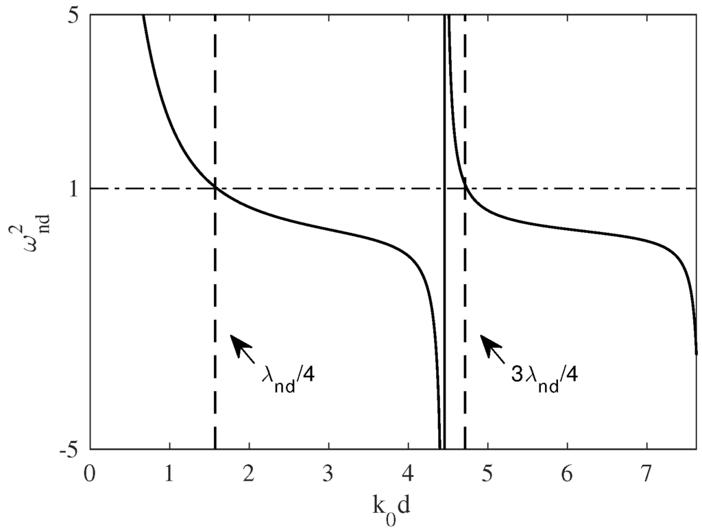
Figure 9.
Dimensionless frequency vs. dimensionless chamber length. Solid line, ; vertical dashed lines, and .
Figure 10a lists the variations with chamber length d. The peak capture factors are observed at different wave periods corresponding to the nodal points of the standing waves as explained above. Zero is seen at the corresponding anti-nodes. It is evident that the flap needs to be placed at a node at which the horizontal water particle velocity is predominant. At about the second peak region (relative to the wave period), where the device in this study is tuned, the bandwidth frequency is rather high. The curve gradient at lower wave period side also is higher than that of the higher wave period side. Therefore, in the design/tuning the device these features should be considered by setting the dominant frequency on the the higher side. Figure 10b indicates variations in the with the change in distance from the hinge point to the free water surface l (for same ). In this instance, small changes are noted in the peak period but without any critical effect to the system. Figure 10c shows the variations with the tide. A significant shift of about 1 s per 0.5 m change to the peak wave period of the tide can be seen.
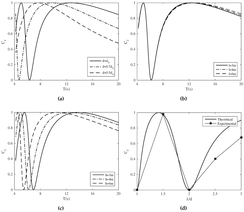
Figure 10.
Variation of capture factor (Cf) with wave period (T), for variable (a) d, (b) l, (c) h, and (d) experimental [31] and theoretical comparison of Cf with normalized wave length (λ/d).
Figure 10d shows the comparison of the theoretical results from this study and the experimental results recorded by Murakami et al. [31] for the capture factor with the normalised wave length . Here, only the comparable experimental results with the Pendulor device from the floating pendulum experiments were extracted, where the floater remains almost stable in the range of = 1 to 2. The floater oscillations are significant beyond that region and therefore the is considerably decreased. The experimental results concur well with the theoretical results when the floating pendulum device behaves as the fixed Pendulor device.
Figure 11a indicates the variation of with wave period (T) for different PTO system damping (N). Figure 11b shows the variation of the amplitude of oscillations () for the same. The maximum of 1 reaches only when as expected at the resonance wave period of 12 s. Anyhow, values correspond to larger damping get little higher for wave periods around the anti-node. It can be understood by the power capture which is proportional to the PTO damping and the square of amplitude of oscillation. According to Figure 11b, around the anti-node, the changes in the damping value does not significantly influence to the variations of the amplitude of oscillations. Therefore, higher damping values give higher at the corresponding wave periods.
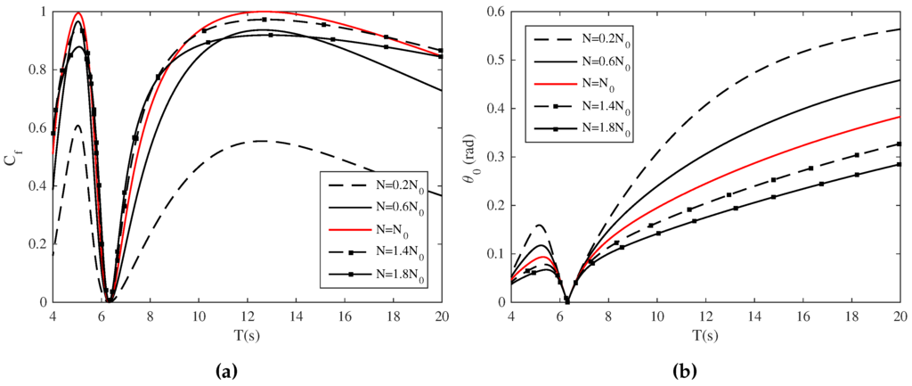
Figure 11.
(a) Variation of capture factor (Cf) and (b) Amplitude of angle of oscillations (θ0), with wave period (T), for different PTO system damping (N).
3.1.2. Coulomb Damping
In order to assess the optimum frictional torque , an equivalent frictional toque was attained by equating the half-cycle energy dissipation of the linear damper at the optimal tuned condition [32] as seen in Equation (28). Here the reference value of was taken for the regular 12 s wave period and the 1.35 m wave height (in this case, Nm assessed by employing Equation (28)).
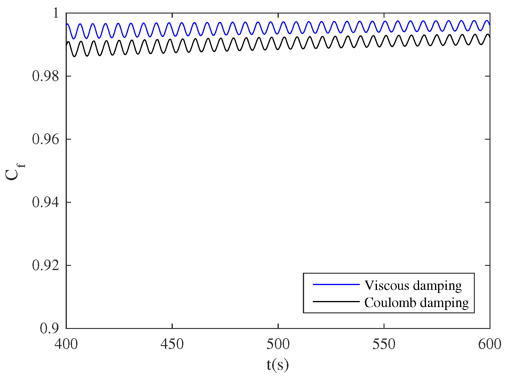
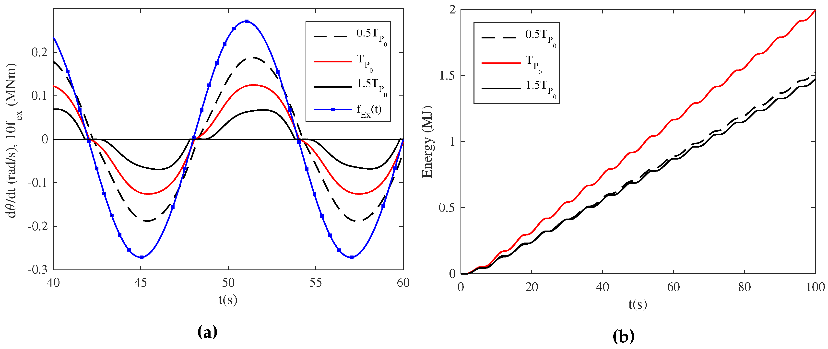
Figure 12 shows the time averaged (calculated as: (cumulative output energy up to a particular instant)/ (average wave power × time)) for both types of damping models for regular waves. The was decreased by about 1% compared with the linear damping model at the steady state operating condition. Figure 13a shows angular velocity variations with time under regular wave conditions. A minor latching effect was evident which causes an expected drop in the efficiency. A further increase in the torque (line corresponds to ) reveals a more dominant latching effect where the flap remains for some time until the wave-induced torque is more than the torque needed to move the flap . Figure 13b reveals the cumulative energy capture with times for the different loading torque conditions and when the loading torque is equivalent to the the maximum power capture is attained.
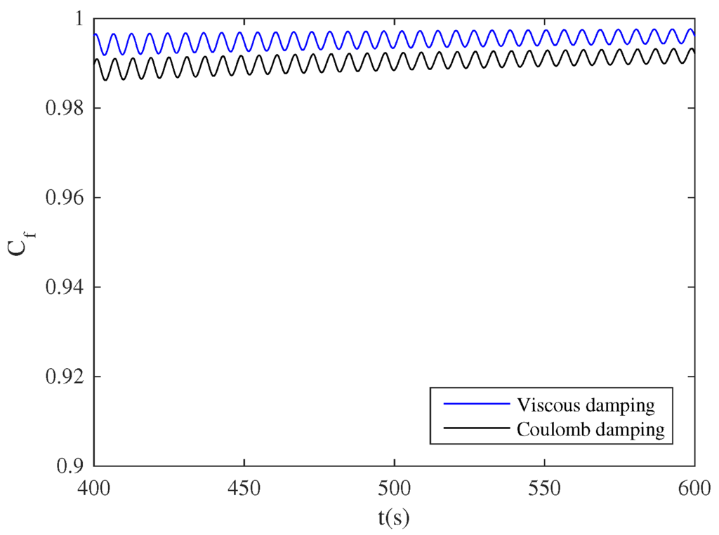
Figure 12.
variation between the linear (viscous) and coulomb damping models (blue line: for linear (viscous) damping; black line: for Coulomb damping).

Figure 13.
(a) Phase difference of fEx vs. and (b) Cumulative energy capture for different loads with time.
3.2. The Case of Irregular Waves
To study the device performance in the real sea state, the device features are simulated by computer generated irregular waves. The Pierson Moskowitz type spectral distribution is employed to approximate the wave spectra for the fully developed wind waves [33]. The spectrum observed in Equation (29) which best matched the Sri Lankan south coastal wave climate [34] has been incorporated, in which is the significant wave height and the significant wave period.
For comparison purposes, the for the irregular waves were also defined using the spectral power of the incoming waves.
where is the power absorbed by the device and is the power available in the irregular wave spectrum. Both terms can be expressed as a simplified version of Rusu [35] as follows:
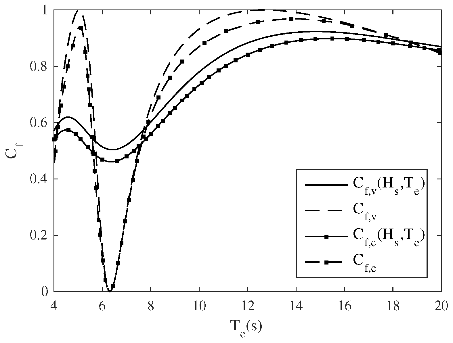
where, is the power absorbed at frequency ω and can be expressed as . Where, is the device capture factor (Equation (7)) when a regular wave of frequency ω approaches the device which is tuned at the wave period and wave height . In fact, indicates the power of a wave at a single frequency chosen from the spectrum and is equal to where is the group velocity and . For shallow water . Using the analysis given above and the frequency domain results, Figure 14 shows the spectral performance of the device under both regular and irregular wave conditions. The dashed lines indicate the regular wave variations for both damping conditions. The solid lines represent the for the irregular waves for both damping conditions. Any representative point on the solid curve (irregular waves) indicates the maximum at that specific significant wave period (because there is a spectrum corresponding to that point) when the PTO damper is adjusted to utilise the maximum power of each wave in that specific spectrum. Thus, practically, a control strategy must be applied to alter the damping torque correctly to suit each incoming wave. Then, plant optimum control can be attained. Consequently, the maximum = 0.92 is reached in the instance of linear damping for the spectrum selected. Nevertheless, the practical implementation of such optimum control is not easy and several studies are still being done in this regard [36].

Figure 14.
Spectral performance of the plant (solid lines indicate spectral and the dashed lines show the of a regular wave).
Figure 14 reveals the wave period at peak for the irregular waves (solid curves) which are moved to a higher value than the one corresponding to the regular wave (dotted curves). This is because of the lower steepness of the gradient of the curve at higher wave periods (i.e., after 12 s) compared with the lower wave periods (i.e., before 12 s). This also means that the majority of the waves in the spectrum come under the higher efficiency range. Therefore, this feature can be utilised positively to decrease the chamber length (tuning the plant for a lower wave period/wave length) than which is relevant to the specific significant wave period. Quantitative analysis like this needs to be meticulously done as such features are highly dependent on the type of the wave spectrum. A deeper analysis on this subject is given in Section 3.3.
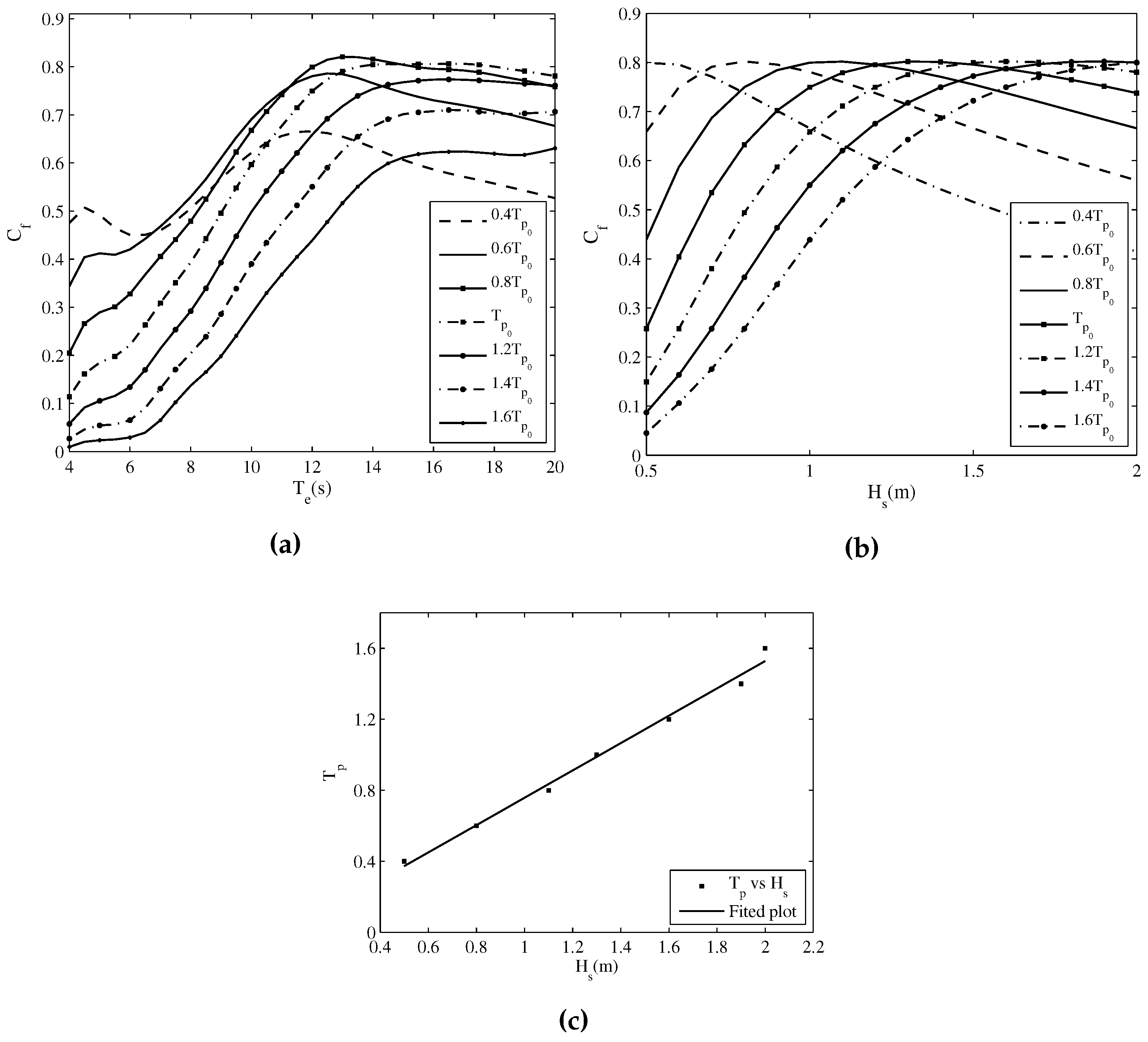
Figure 15a reveals the variations with the significant wave period for different loading conditions without any control strategy being done. In this instance, the Coulomb damping model is employed with the device tuned at = 12 s and = 1.35 m where the wave height corresponds to 1 m wave height in deep water. The maximum at the significant 12 s wave period is attained when the device is tuned at = 0.8. Figure 15b shows the variations with at the significant 12 s wave period, implying that the maximum remains unchanged with the incoming wave height. In order to maintain the at the higher level, the must be correctly adjusted. Figure 15c shows the variation with when maximum is attained at = 12 s. As the and are almost linearly proportional, the device can operate even at higher efficiencies by utilising a proportional controller. This can be practically implemented as suggested by Watabe et al. [37].

Figure 15.
Variation of Cf with (a) Te; (b) Hs for different loading conditions; and (c) Optimum loading conditions for maximum Cf for different Hs.
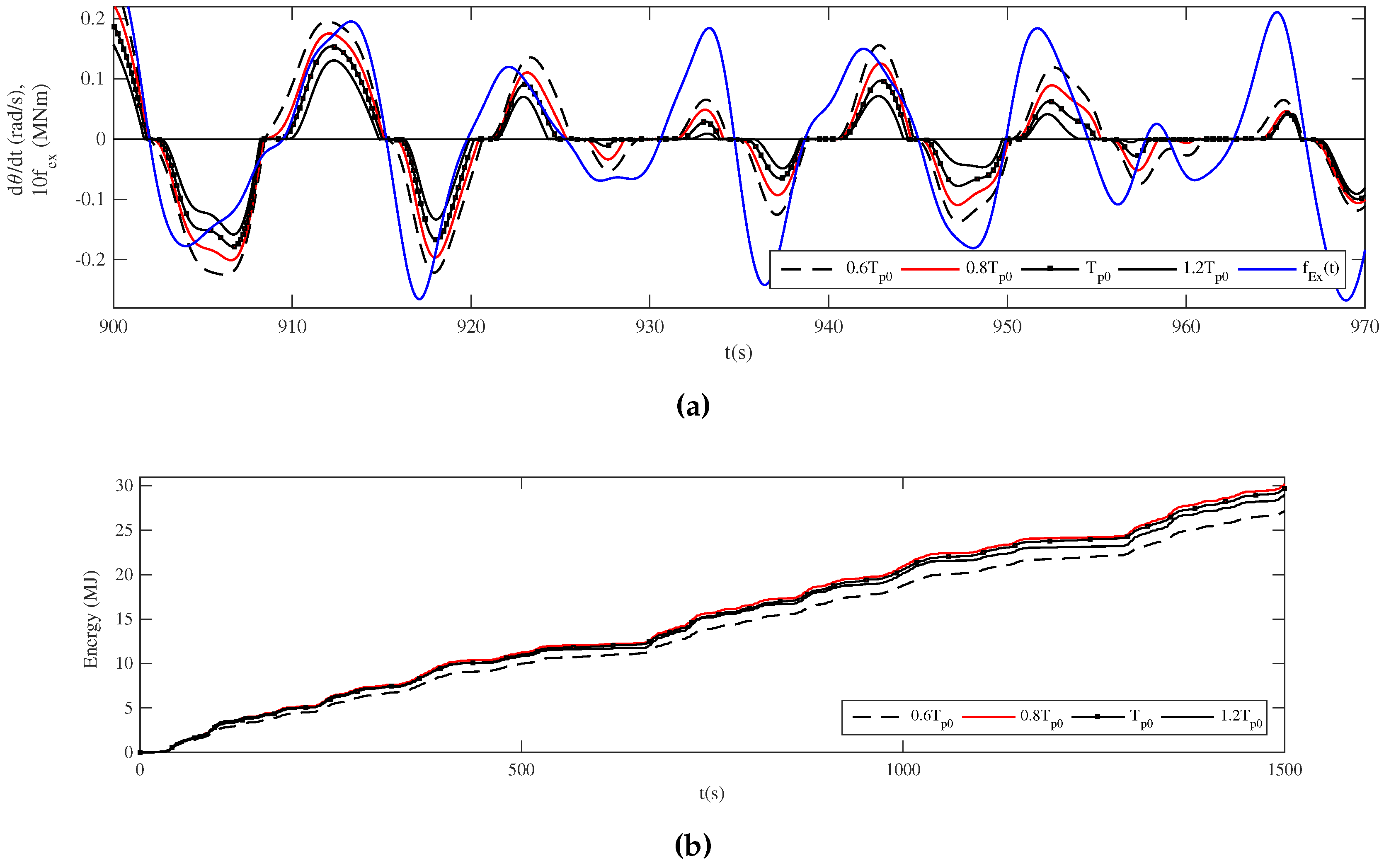
Figure 16a reflects variations in the angular velocity of the flap and wave excitation moment for different loading conditions. Figure 16b shows the cumulative energy capture for a 1500 s period for the same, demonstrating that the maximum energy is yielded when the load torque is at 0.8. Under identical conditions, the maximum energy yield for a regular wave is attained when the loading condition is tuned at = (as seen in Figure 13b). This is because the regular waves have power greater than the spectral power of the irregular waves for the spectrum chosen. Figure 16a, the latching behaviour of the flap is observed for different loading conditions and the corresponding stages with the incoming wave. All the curves linked to flap velocity are not significantly in phase with the waves as there is no optimum controller. When device is at the maximum energy yield setting (), the flap oscillations follow the phase comparatively closely.
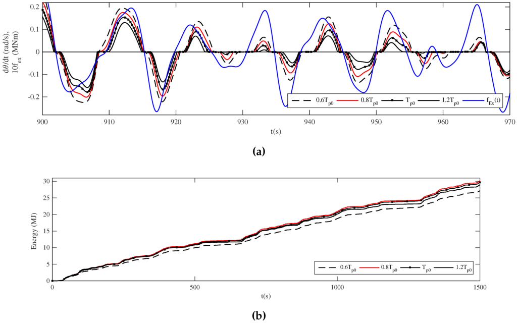
Figure 16.
(a) Variation of angular velocity of the flap and wave excitation moment for different loading conditions; (b) Cumulative energy capture with time.
3.3. Influence of the Chamber Length
A considerable part of the construction cost of the “Pendulor” wave energy device is mainly due to the caisson erection. The caisson size is mostly dependent on the chamber length; therefore, the influence of a decrease in the chamber length on the performance is discussed in this Section.
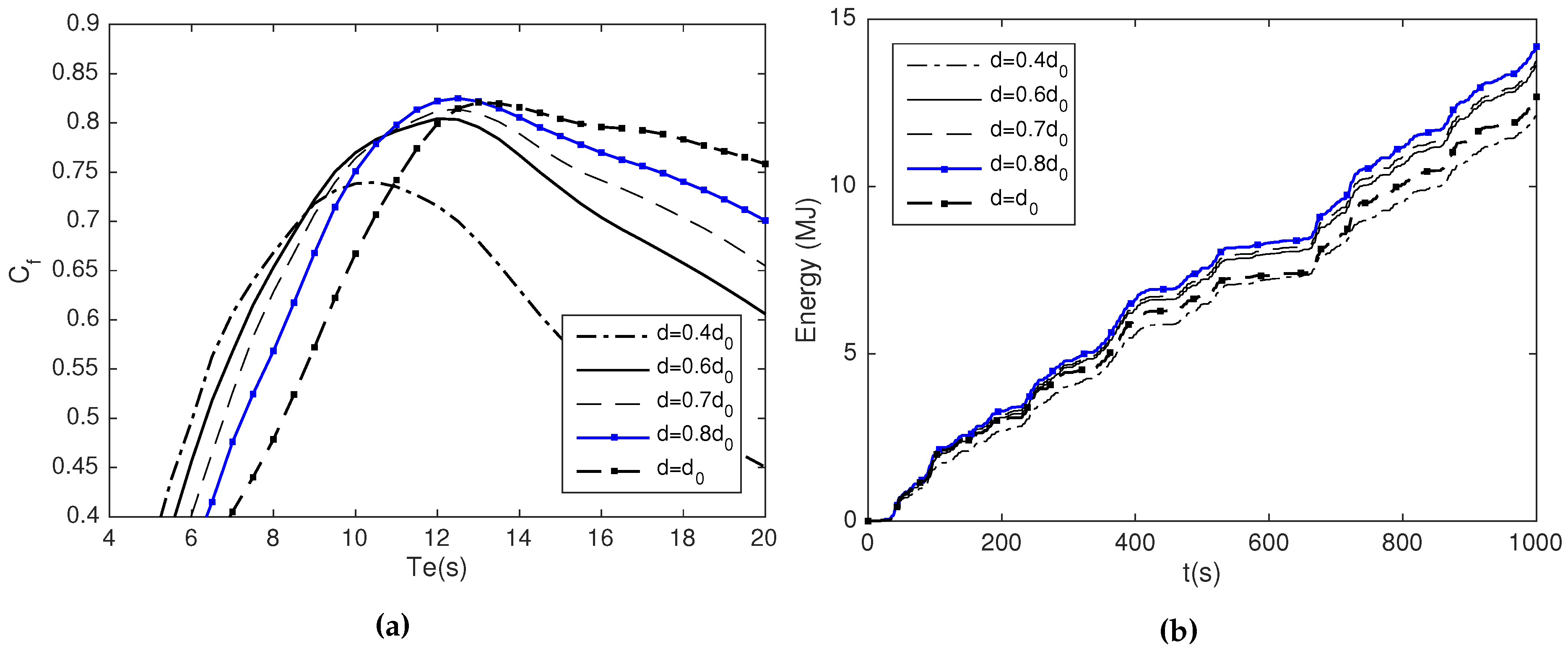
Figure 17 reveals the variations for the different chamber lengths (d) at the optimal control condition as given in Section 3.1.2. The results indicate that the peak efficiency corresponds to the significant 12 s wave period which happens when d = 0.7 to 0.8. This, thus implies that there is a prospect to reduce the chamber length. In Figure 18a, variations are seen with significant wave period for the different chamber lengths without any controller. When d = 0.8, the maximum is seen at = 12 s. The corresponding spectral characteristic of the curve () also covers a wide range of significant wave periods quite well when compared with the other curves. Figure 18b shows the cumulative energy capture at = 12 s by varying the chamber lengths. The three curves corresponding to the chamber lengths , 0.8 and 0.6 closely follow one another. Of them 0.8 shows the maximum energy capture and 0.6 is also very similar to the same. This is an indication that the chamber length can be reduced even more by a further 20% to d = 0.6 by compromising only around 4% of the energy yield, if it is economically feasible. Therefore, there is a potential to reduce the chamber length by sacrificing a small fraction in the energy yield.
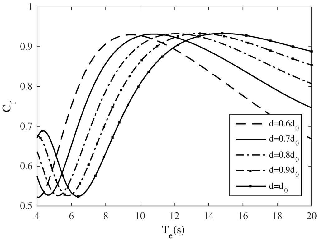
Figure 17.
for different chamber lengths in the optimal control condition with (s).
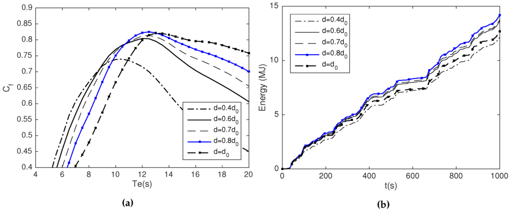
Figure 18.
(a) Cf variation with Te s for varies values of d s without any controller; (b) Cumulative energy capture at Te = 12 s by varying the chamber lengths.
4. Discussion
A numerical model of the Pendulor device has been developed for a better understanding of the behavior of the device under regular and irregular wave conditions when the flaps are configured in an array arrangement. A maximum primary conversion efficiency of about 80% was seen for the irregular waves (selected wave spectrum) without using any optimal or sub optimal control strategies. Sea trials performed for similar Pendulor devices have also revealed high energy capture efficiency between 40 % and 60 % for devices tuned for important wave climatic conditions [4]. Viscous effects, drag forces, wave diffraction (at the ends of the Pendulor array system), wave directional and breaking properties (site specific), and point absorbing effects (quasi-point absorbing effect) were not taken into consideration in our work. Consideration of these factors increase the complexity of the analysis and remains as a future direction to be pursued.
The Pendulor device has the distinctive advantage of having the ability to match its natural frequency () by setting the design parameters comparatively more easily than that of the point absorbers and unbounded flap devices. This is because, the chamber effect generates sufficient spring constant via the chamber side restoring the coefficient (i.e., ). Therefore, the tuned device reveals the broader bandwidth of in its primary energy conversion phase. As discussed in Section 3.1.1, the other crucial parameter is the chamber length d, which is easily assessed by the significant wave length. Using such basic analysis, it is possible to get the fundamental design parameters for the Pendular device. The designed system was simulated as such in the irregular wave environment and fairly broader above 0.5 were obtained (refer Figure 18a). In this study, the features of the load torque that are implicitly dependent on the HST system loaded with the accumulator pressure/flow control systems [23,37] have not been considered. Therefore, to further enhance the energy yield, the only available controllable parameter is the load torque according to the model proposed. Therefore, via appropriate load control, the performance could be raised at varying sea states. Falcão [38] had investigated this approach by phase control via load control while varying the load applied to the PTO to raise the competence of the point absorbers. Similar types of approaches are possible in this case also. Further, Watabe et al. [37] proposed an HST system with an autonomous optimum controller for the Pendulor device control. Further studies are required before implementing such control methods for greater performance enhancement.
As stated earlier on, one of the major factors affecting the performance is chamber length, where one-quarter of the wave length results in enormous constructional expenses and related issues. Therefore, a considerable decrease in the chamber length needs to be considered as a leading requirement. Many preliminary studies have been performed for this and changing the chamber shape was found to possibly reduce the length by about 30% for regular wave applications [10]. Further, Folley et al. [39] emphasised that, for the top-hinged flap type devices in the shallow waters, the power capture was related more to the incident wave forces than to the incident wave power. These studies showed that the wave surging in the area of the flap controls the device characteristics. Thus, the caisson must be designed in a manner that effective surge would happen in the vicinity of the flap while retaining the proper restoring effect () on the chamber side. Further, as a result of this work, it was found that it is possible to reduce the chamber length by 20%–40% for the selected wave spectrum utilized for the irregular waves. At any rate, further practical investigations are required to clearly quantify such enhancements.
5. Conclusions
Applying the regular wave theories the numerical model of the “Pendular” wave energy converter, in an array configuration, was developed in an array configuration for irregular wave conditions. Two methods of time domain identification and frequency domain identification were utilised to save computational time while incorporating the modified Cummins equation in the model. The identification accuracy agrees well with the analytical results.
Parametric analysis was done based on the numerical model, in order to identify the influence of the major geometrical and wave climatic parameters which could affect the capture factor. The distance from the back wall to the flap location and tidal differences were identified as the factors most influencing the capture factor. As tidal changes are beyond human control their effect on device performance must be carefully addressed in the stages of design, operation and control. It was shown that, about a maximum primary capture factor of 0.8 can be achieved by tuning the basic parameters of chamber length and power take-off damping torque without the use of any control strategy. Furthermore, the capture factor is shown a broader bandwidth of more than 0.5 throughout the 4 to 20 s wave periods.
The distance from the back wall to the flap position (chamber length), normally one-quarter of the wave length, can be further reduced by about 20% without incurring any energy loss. A further 20%–40% of chamber length can be decreased by compromising 0%–4% energy capture if it is economically feasible. Hence, because the potential to reduce the caisson size is substantial, it will facilitate a significant reduction in the total construction cost. Such quantitative values are dependent upon the wave climate at the specific site as well as the other device design parameters. Therefore, the results of this study will be useful in the estimation of the device parameters and evaluation of the performance under irregular wave conditions.
Acknowledgments
This work is carried out as a part of the research work under the grant RG/AF 2013/30E by University of Peradeniya, Sri Lanka. Authors are also grateful to the reviewers of this paper for their helpful comments.
Author Contributions
Sudath Prasanna Gunawardane supervised the main theme of this paper and prepared the manuscript by interpreting the results. Chathura Jayan Kankanamge developed and simulated the theory, and produced the results. Tomiji Watabe continually contributed to the study through his thoughts on practical aspects and reviewed the outcome.
Conflicts of Interest
The authors declare no conflict of interest.
Abbreviations and Notations
The following abbreviations are used in this manuscript:
| FDI | frequency domain identification |
| OWC | oscillation water column |
| OSWC | oscillating Surge Wave Converter |
| PTO | power take off system |
| SSM | state space models |
| TDI | time domain identification |
| TF | transfer function |
imaginary part of the radiation impedance | |
frequency dependent radiation moment (real part of the radiation impedance) | |
| b | width of the flap |
group velocity | |
capture factor | |
| d | Chamber length (length from flap tp back wall of the flap) |
non-dimensional chamber length | |
effective chamber length (when plant tuned at T = 12 s) | |
buoyancy moment | |
drag moment on the flap | |
excitation moment | |
hydro dynamic and static moments applying on the flap | |
restoring moment due to mass of the flap | |
external mechanical torque on the flap | |
radiation moment | |
| g | acceleration due to gravity |
| H | amplitude of the incoming wave |
significant wave height | |
| h | water depth of the chamber |
moment of inertia of the flap | |
| I | frequency dependent added inertia |
| k | hydrostatic restoring coefficient |
root of the dispersion relationship | |
restoring coefficient of PTO | |
restoring coefficient due to mass of the flap | |
non-dimensional wave length | |
| l | free surface of water to hinged point of the flap |
length from hinged point of the flap to gravity centre of the flap | |
| m | mass of the flap |
| N | damping coefficient of PTO |
absorbed power of the device | |
available power irregular wave | |
time averaged power of incoming wave | |
frequency spectra of the sea | |
| T | time period of the incoming wave |
significant wave period | |
external coulomb damping moment on the flap | |
optimum coulomb damping moment at T = 12 s, and H = 1.35 m | |
impulse response function | |
| θ | angle of oscillation of the flap |
amplitude of angle of oscillation of the flap | |
| ω | frequency (rad/s) |
resonance frequency (rad/s) | |
| ρ | static density of water |
| λ | wave length |
non-dimensional wave length |
Appendix A. 2D potential theory for Pendulor device
Appendix A.1. Velocity Potential
The theory is developed by considering the wave energy device as a wave maker. For an array configurations of Pendulor devices, it is reasonable to assume that the caisson is infinitely long which enables to analyse the problem in 2D.
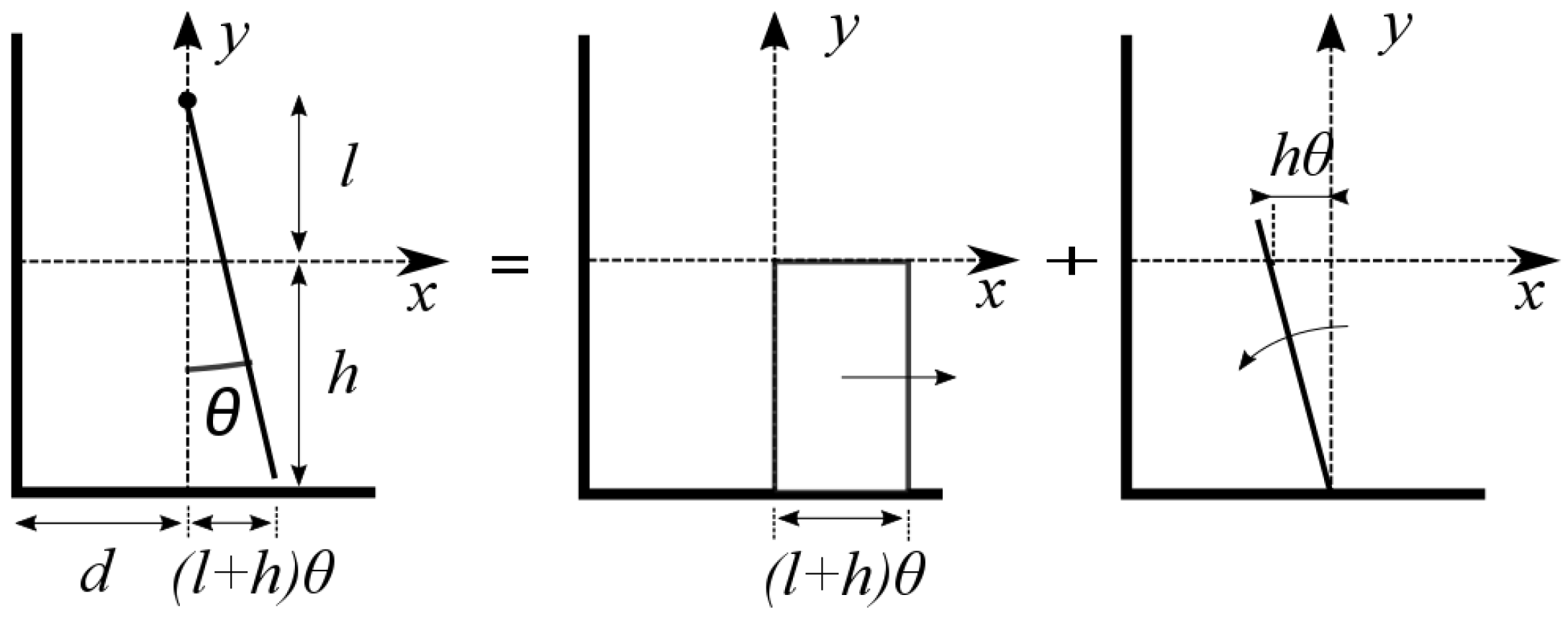
Figure A1 shows the graphical replication of a top hinged flap type wave maker by the superposition of piston type and bottom hinged flap type wave makers. When the piston wave maker moves from its origin to the +ve x direction, the bottom hinged wave maker oscillates counter-clockwise direction and vice versa (here θ is the angle of oscillation of top hinged flap).

Figure A1.
Graphical interpretation of superposition of piston type wave maker and bottom hinged flap wave maker.
Supposing the flap is completely extended to the bottom and tightly fitted to the chamber width, the flow across the flap is assumed to be negligible for smaller angles of oscillations. Also, the fluid is assumed inviscid, incompressible and irrotational. Then the Velocity potential Φ must satisfy Laplace equation:
The Linearized form of dynamic and kinematic free surface [ is the free surface] boundary condition reads:
Here subscripts denotes the differentiation with respect to the relevant variable. The bottom surface of the caisson satisfies the boundary condition as shown in Equation (A3).
For harmonic waves, the velocity potential takes the form of:
where ω is the harmonic frequency and ψ is the spatial velocity potential. Applying Newton’s law to the flap about hinged point, the simplest form of governing equation states:
The divided fluid regions, as described in the main text (see Figure 2), satisfy the boundary conditions mentioned in Equations (A1)–(A3). Since the Laplace equation and boundary conditions are linear, by applying principle of superposition, the velocity potential of the fluid domain can be written as follows by combining sea and chamber side potentials.
where and are the sea side and chamber side velocity potential functions respectively and the corresponding potentials are obtained in Section A.1.1 and Section A.1.2 respectively.
Appendix A.1.1. Sea Side Velocity Potential
As previously mentioned, the equivalent top hinged flap type wave maker effect is modelled by superposition of piston and bottom hinged wave makers. Accordingly, velocity potentials of piston and bottom hinged flap type wave makers described by Deen and Dalrymple [24], are used to obtain the corresponding velocity potentials in this particular analysis.
Therefore, the velocity potential of the piston type wave maker can be obtained as shown in Equation (A7):
where , , is given by the dispersion relationship and . The velocity potential of the bottom hinged flap for sea side is:
Where , Equation (A9) shows velocity potential of the top hinged flap type wave maker by combining piston type and bottom hinged flap type wave makers (for more detailed see Figure A1).
Combining Equations (A7)–(A9), the potential function for sea side can be stated as:
where .
Appendix A.1.2. Chamber Side Velocity Potential
Boundary conditions for the chamber side except the back wall satisfy Equations (A1)–(A3). The boundary condition of the back wall is:
The velocity of the flap in to the x direction is:
For harmonic waves, time component and the spatial component of the velocity potential can be factored out as, . Based on the analysis done by Watabe [7], the velocity potential for both piston type and bottom hinged flap type wave makers with a back wall can be written as follows:
When chamber side velocity potential should take the form of that of the sea side. That can be proved by using exponential functions. Here is a parameter which depends on the boundary conditions. Equation (A14) shows the x coordinate of the bottom hinged flap with respect to the vertical distance y.
Equation (A15) shows the horizontal velocity.
Equation (A16) satisfies the lateral boundary condition and taking the effective terms by using truncated Tailor series [24],
Velocity of the flap to the direction x without the time dependent harmonic is:
Parameter can be simply found by integrating Equation (A17) by [24]. Thus . Therefore, velocity potential of the bottom hinged flap for the chamber side is and it simplifies to:
By using the same method, velocity potential for the piston type wave maker can be obtained and shown in the Equation (A19).
Appendix A.2. Hydrodynamic Parameters of the Device
Hydrodynamic parameters acting on the flap are obtained by decomposing the total moment acting on the flap into the terms of acceleration, velocity, and displacements. They are then separated as added inertia, damping, and restoring coefficient respectively.
Appendix A.2.1. Chamber Side Hydrodynamic Parameters
The fluid pressure in the chamber side is:
Therefore, the moment acting on the flap about the hinged point can be stated as:
Thus becomes:
Equation (A23) can be decomposed as:
also, can typically be written as:
Where is the hydrodynamic added inertia, is the radiation damping coefficient and is the hydrostatic restoring coefficient. In order to find taking limiting value (very slow motion of the flap) in Equations (A24) and (A25).
Appendix A.2.2. Sea Side Hydrodynamic Parameters
The analysis for the sea side can be done similarly as described in the above section. Thus, the moment acting on the flap due to sea side wave action, can typically be written as:
Then the added inertia, the radiation damping and the hydrostatic restoring coefficient can be found as below:
Appendix A.2.3. Excitation Moment
To obtain the excitation moment acting on the flap due to incident waves, the characteristics waves generated by the flap when is considered. The moment acting on the flap is formulated when the flap is in fixed condition. Then the incoming wave reflects at the flap and standing wave is generated. The velocity potential of the standing wave is therefore,
Using the similar method stated in the Section A.2.1, excitation moment is formulated as bellow:
where
The free surface elevation of the standing wave is:
The maximum height of the standing wave should be twice that of the incoming wave height H. Therefore can be found as:
is the amplitude of oscillation of the flap.
References
- Watabe, T.; Kondo, H.; Matsuda, T.; Yano, K.; Dote, Y.; Takagi, M. Method and Apparatus for Generating Electric Power by Waves. U.S. Patent 4,490,621, 25 December 1984. [Google Scholar]
- Watabe, T. “Pendulor” wave power converter—Fifteen years study and future prospect. In Proceedings of the International Symposium on Ocean Energy Development for Overcoming the Energy & Environmental Crises, Muroran, Hokkaido, Japan, 26–27 August 1993; pp. 41–52.
- Watabe, T.; Kondo, H.; Shirai, H.; Seino, K. Re-modeling of Muroran wave test plant. In Proceedings of the Forth International Offshore and Polar Engineering conference, Osaka, Japan, 10–15 April 1994; Volume 1, pp. 353–358.
- Watabe, T.; Yokouchi, H.; Kondo, H.; Inoya, M.; Kudo, M. Installation of the new “Pendulor” for the 2nd stage sea test. In Proceedings of the Ninth International Offshore and Polar Engineering Conference, Brest, France, 30 May–4 June 1999. Number ISOPE-I-99-021.
- Watabe, T.; Kondo, H. A new rotary vane pump for ocean wave power conversion. In Proceedings of the 2nd International Symposium on Fluid Power Transmission and Control ISFP’95, Shanghai, China, 5–7 October 1995; pp. 48–52.
- Kondo, H.; Watabe, T.; Yano, K. Wave power extraction at coastal structure by means of moving body in the chamber. Coast. Eng. 1984, 1, 2875–2891. [Google Scholar]
- Watabe, T. Utilization of the Ocean Wave Energy; Fuji Print Company Ltd.: Muroran, Japan, 2007. [Google Scholar]
- Park, J.; Shin, S.; Hong, K.; Kim, S. A study on the wave response and efficiency of a pendulum wave energy converter. In Proceedings of the Twenty-second International Offshore and Polar Engineering Conference, Rhodes, Greece, 17–22 June 2012; pp. 601–606.
- Folley, M.; Whittaker, T.; Osterried, M. The oscillating wave surge converter. Int. J. Offshore Polar Eng. 2004, 1, 1–5. [Google Scholar]
- Gunawaradane, S.D.G.S.P.; Abeysekara, M.P.; Uyanwaththa, D.M.A.R.; Tennakoon, S.B.; Wijekoon, W.M.J.S.; Ranasinghe, R.A.P.C. Model study on “Pendulor” type wave energy device to utilize ocean wave energy in Sri Lanka. In Proceedings of the International Conference on Sustainable Built Environment (ICSBE-2010), Kandy, Sri Lanka, 13–14 December 2010; pp. 297–303.
- Watabe, T.; Yokouchi, H.; Gunawardane, S.; Obeyesekera, B.; Dissanayake, U. Preliminary study on wave energy utilization in Sri Lanka. In Proceedings of the Eleventh International Offshore and Polar Engineering Conference, Stavanger, Norway, 17–22 June 2001; Volume I, pp. 596–603.
- Ferri, F.; Ambühl, S.; Fischer, B.; Kofoed, J.P. Balancing power output and structural fatigue of wave energy converters by means of control strategies. Energies 2014, 7, 2246–2273. [Google Scholar] [CrossRef]
- Cummins, W.E. The Impulse Response Function and Ship Motions. 1962. Available online: https://dome.mit.edu/handle/1721.3/49049 (accessed on 6 April 2016).
- Taghipour, R.; Perez, T.; Moan, T. Hybrid frequency-time domain models for dynamic response analysis of marine structures. Ocean Eng. 2008, 35, 685–705. [Google Scholar] [CrossRef]
- Duarte, T.; Sarmento, A.; Alves, M.; Jonkman, J. State-space realization of the wave-radiation force within FAST. In Proceedings of the ASME 2013 32nd International Conference on Ocean, Offshore and Arctic Engineering, Nantes, France, 9–14 June 2013.
- Chen, M.; Eatock, R.; Sang, Y. Time domain modeling of a dynamic impact oscillator under wave excitations. Ocean Eng. 2014, 76, 40–51. [Google Scholar] [CrossRef]
- Zhang, X.; Yang, J. Power capture performance of an oscillating-body WEC with nonlinear snap through PTO systems in irregular waves. Appl. Ocean Res. 2015, 52, 261–273. [Google Scholar] [CrossRef]
- Amarasekara, H.W.K.M.; Abeynayake, P.A.G.S.; Fernando, M.A.R.M.; Atputharajah, A.; Uyanwaththa, D.M.A.R.; Gunawardane, S.D.G.S.P.; Gerdin, L.; Keijser, M.; Fåhraeus, M.W.; Fernando, I.M.K.; et al. A prefeasibility study on ocean wave power generation for the Southern Coast of Sri Lanka: Electrical feasibility. Int. J. Distrib. Energy Resour. Smart Grids 2014, 10, 79–93. [Google Scholar]
- Falnes, J. Ocean Waves and Oscillating Systems: Linear Interaction Including Wave Energy Extraction; Cambridge University Press: Cambridge, UK, 2002. [Google Scholar]
- Budal, K.; Falnes, J. Interacting Point Absorbers with Controlled Motion. In Power from Sea Waves; Count, B., Ed.; Academic Press: London, UK, 1980; pp. 381–399. [Google Scholar]
- Costa, P.R.; Garcia-Rosa, P.B.; Estefen, S.F. Phase control strategy for a wave energy hyperbaric converter. Ocean Eng. 2010, 37, 1483–1490. [Google Scholar] [CrossRef]
- Perez, T.; Fossen, T.I. Practical aspects of frequency-domain identification of dynamic models of marine structures from hydrodynamic data. Ocean Eng. 2011, 38, 426–435. [Google Scholar] [CrossRef]
- Falcão, A.F.D.O. Modelling and control of oscillating-body wave energy converters with hydraulic power take-off and gas accumulator. Ocean Eng. 2007, 34, 2021–2032. [Google Scholar] [CrossRef]
- Deen, R.G.; Dalrymple, R.A. Water Wave Mechanics for Engineers and Scientists; World Scientific Publishing Co. Pte. Ltd.: Singapore, Singapore, 2000; Volume 2. [Google Scholar]
- Anami, K.; Ishii, N.; Knisely, C.W. Added mass and wave radiation damping for flow-induced rotational vibrations of skinplates of hydraulic gates. J. Fluids Struct. 2012, 35, 213–228. [Google Scholar] [CrossRef]
- Lewandowski, E.M. The Dynamics of Marine Craft Maneuvering and Seakeeping; World Scientific Publishing Co. Pte. Ltd.: Singapore, Singapore, 2004; p. 420. [Google Scholar]
- Porter, R.; Biggs, N.R.T. Wave Energy Absorption by a Flap-Type Oscillating Wave Surge Converter. University of Bristol–Department of Mathematics–Study. Available online: http://www.maths.bris.ac.uk/marp/publications.html (accessed on 6 April 2016).
- Zurkinden, A.S.; Ferri, F.; Beatty, S.; Kofoed, J.P.; Kramer, M.M. Non-linear numerical modeling and experimental testing of a point absorber wave energy converter. Ocean Eng. 2014, 78, 11–21. [Google Scholar] [CrossRef]
- Ogilvie, T. Recent progress towards the understanding and prediction of ship motions. In Proceedings of the Fifth Symposium on Naval Hydrodynamics, Bergen, Norway, 10–12 September 1964.
- MATLAB User Manual; The MathWorks Inc: Natick, MA, USA, 2014.
- Murakami, T.; Imai, Y.; Nagata, S. Experimental study on load characteristics in a floating type pendulum wave energy converter. J. Therm. Sci. 2014, 23, 465–471. [Google Scholar] [CrossRef]
- Beards, C.F.; Eng, C. Structural Vibration: Analysis and Damping; Halsted Press, an imprint of John Wiley & Sons Inc: New York, NY, USA, 1996; p. 287. [Google Scholar]
- Goda, Y. Random Seas and Design of Maritime Structures; World Scientific Publishing Co. Pte. Ltd.: Singapore, Singapore, 2000; Volume 15, p. 443. [Google Scholar]
- Scheffer, H.; Fernando, K.; Fittschen, T. Directional Wave Climate Study South-West Coast of Sri Lanka Report on the Wave Measurements off Galle; Sri Lankan–German Cooperation CCD-GTZ Coast Conservation Project: Colombo, Sri Lanka, 1994. [Google Scholar]
- Rusu, E. Evaluation of the wave energy conversion efficiency in various coastal environments. Energies 2014, 7, 4002–4018. [Google Scholar] [CrossRef]
- Wang, L.; Isberg, J. Nonlinear passive control of a wave energy converter subject to constraints in irregular waves. Energies 2015, 8, 6528–6542. [Google Scholar] [CrossRef]
- Watabe, T.; Yokouchi, H.; Gunawardane, S.D.G.S.P.; Thakker, A. Autonomous optimization control and the controllor for “Pendulor”. In Proceedings of the JFPS International Symposium on Fluid Power, Nara, Japan, 12–15 November 2002; pp. 843–848.
- Falcão, A.F.D.O. Phase control through load control of oscillating-body wave energy converters with hydraulic PTO system. Ocean Eng. 2008, 35, 358–366. [Google Scholar] [CrossRef]
- Folley, M.; Whittaker, T.J.T.; Henry, A. The effect of water depth on the performance of a small surging wave energy converter. Ocean Eng. 2007, 34, 1265–1274. [Google Scholar] [CrossRef]


© 2016 by the authors; licensee MDPI, Basel, Switzerland. This article is an open access article distributed under the terms and conditions of the Creative Commons by Attribution (CC-BY) license (http://creativecommons.org/licenses/by/4.0/).