
Analysis and Optimization of Three-Resonator Wireless Power Transfer System for Predetermined-Goals Wireless Power Transmission


Abstract
:1. Introduction
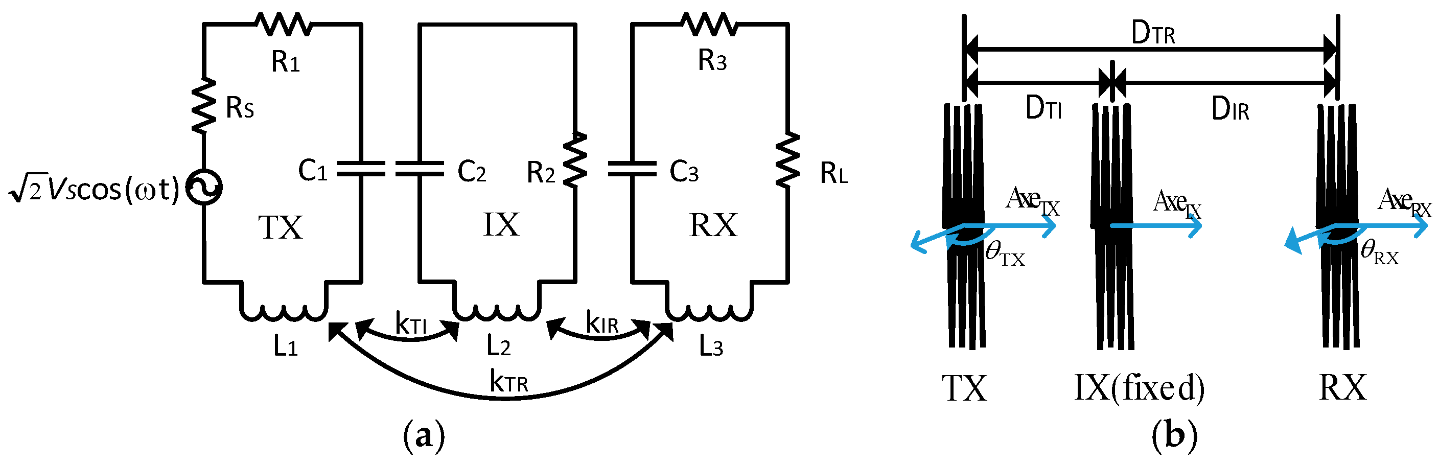
2. System Analysis
2.1. Transfer Characteristics of Power Transfer Efficiency
2.2. Transfer Characteristics of Power Delivered to the Load
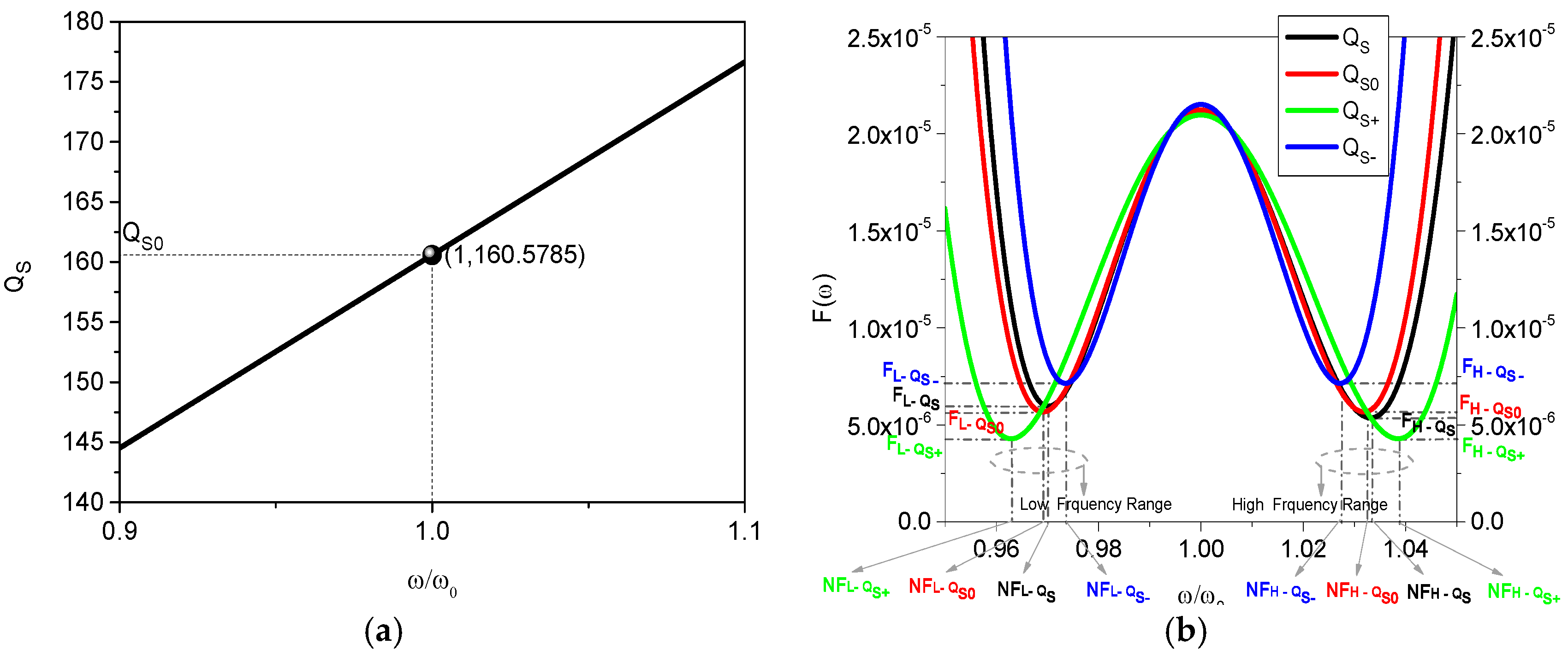
2.3. Theoretical Illumination with a Case Based on Practical Resonators
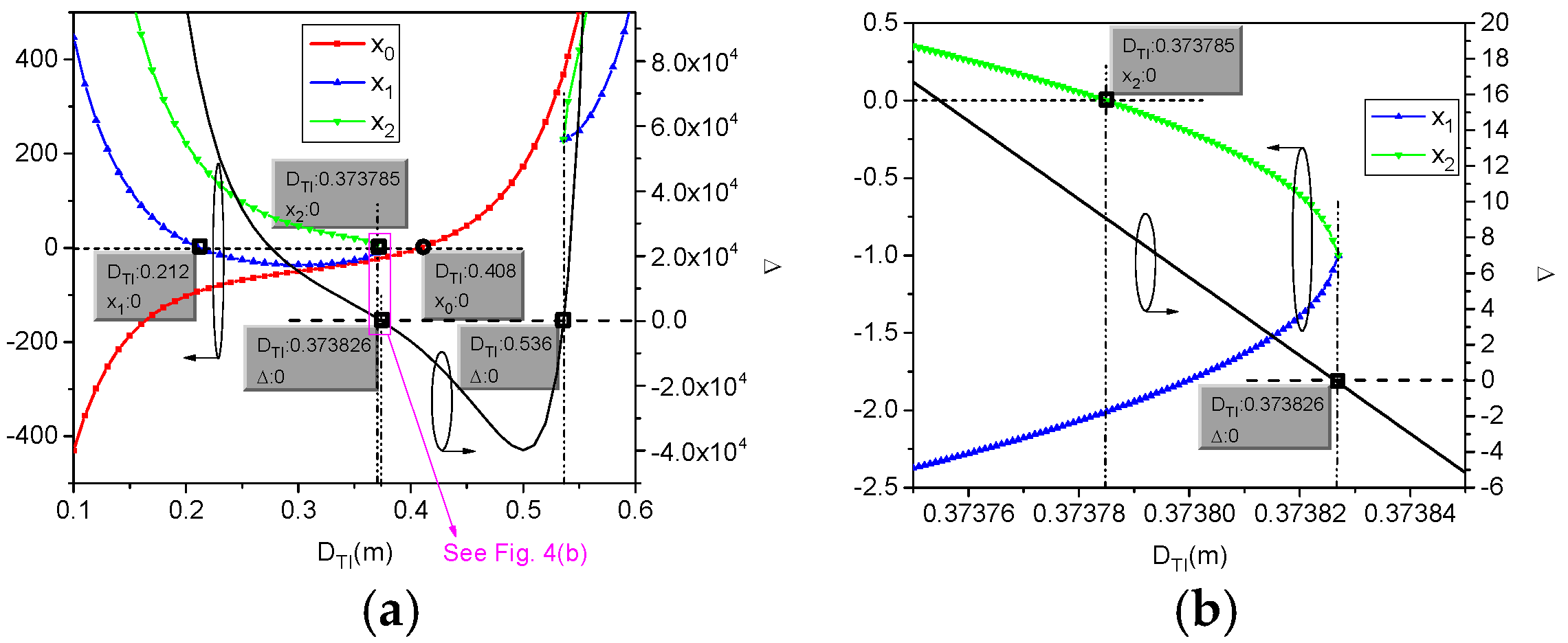
3. Optimization for Predetermined-Goals Wireless Power Transmission
3.1. Setting the Optimization Goals
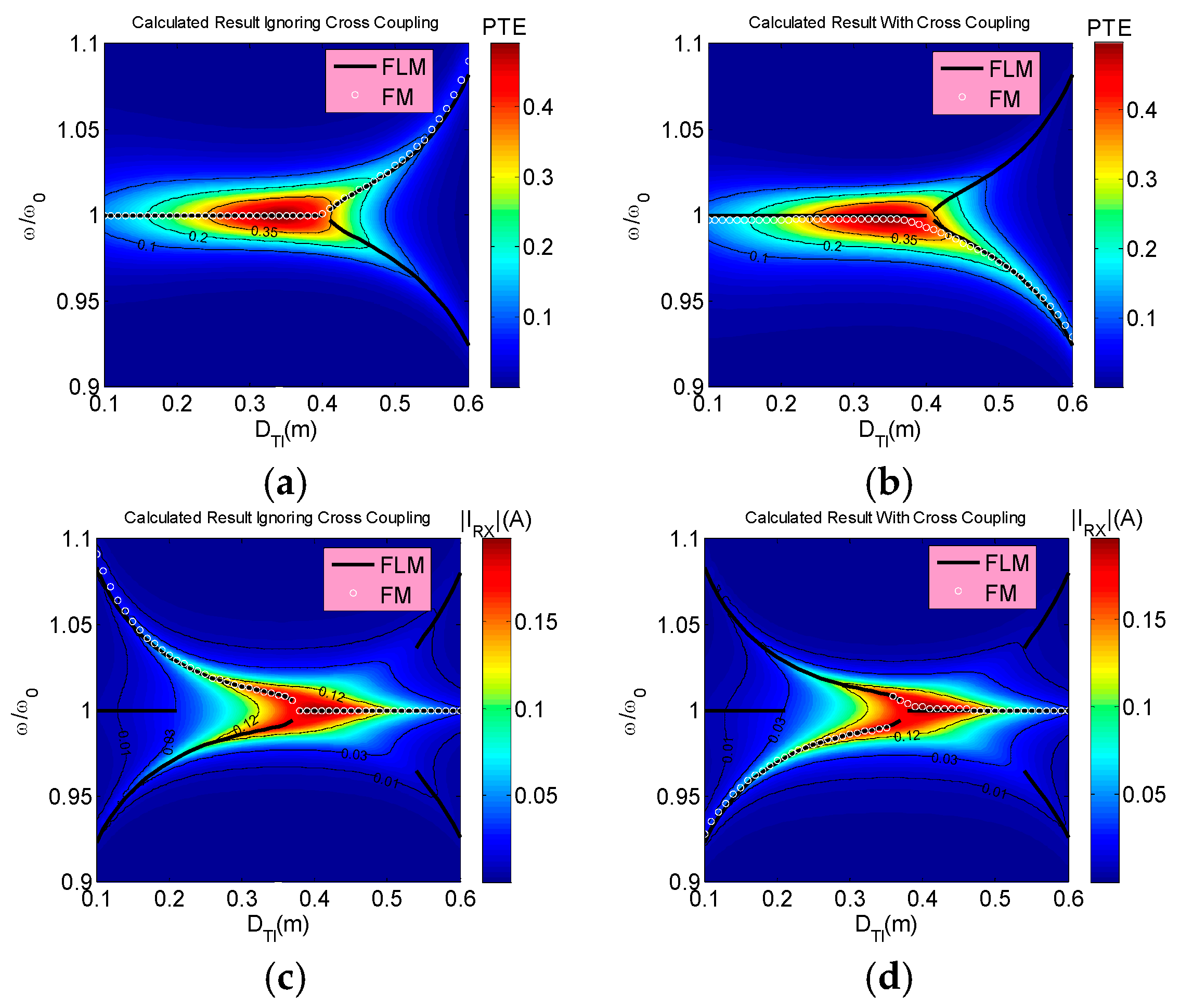
3.2. Numerical Results
4. Experimental Verification
4.1. Experimental Setup
4.2. Measured Results Comparing with Theoretical Values
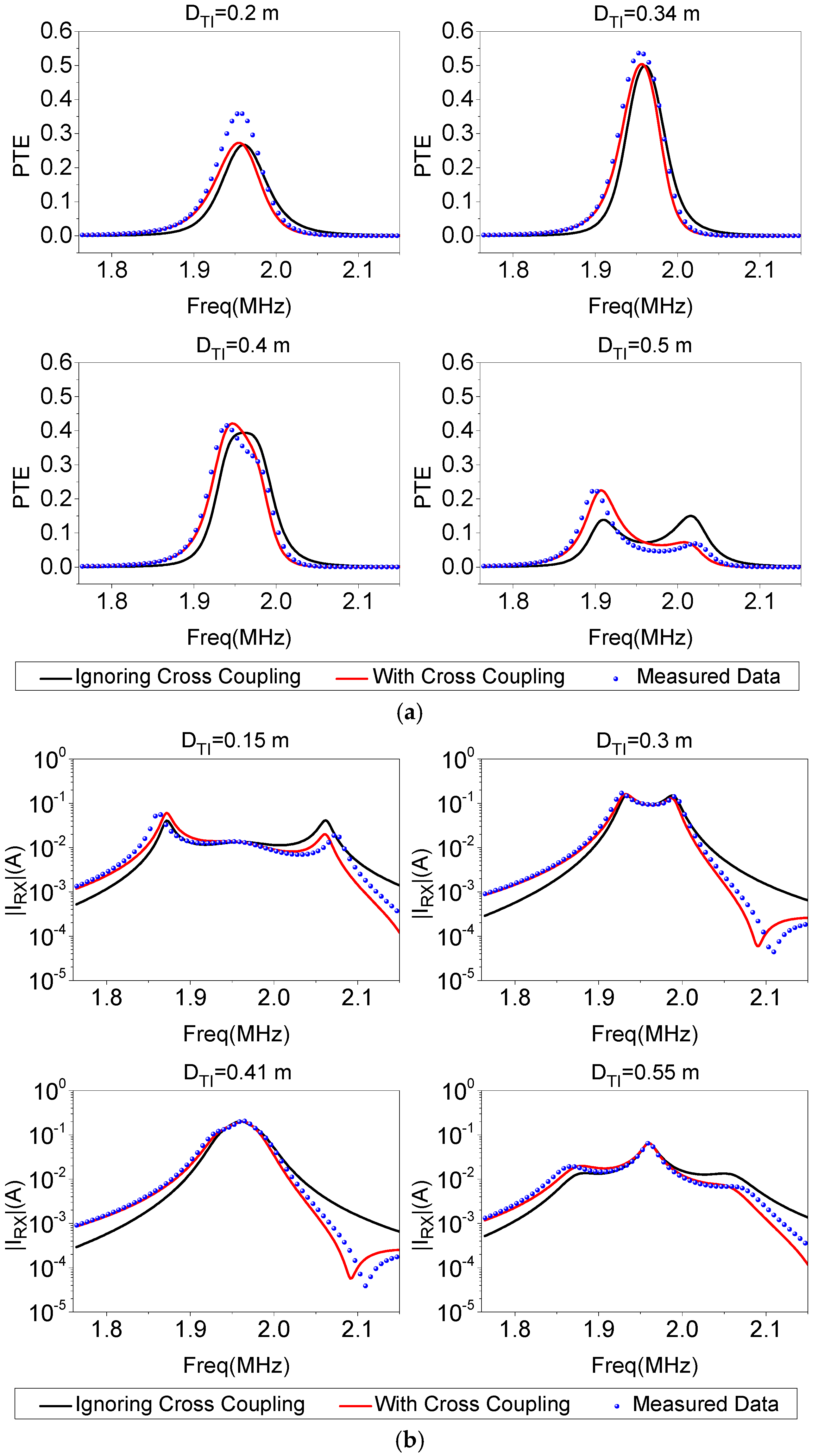
4.2.1. Verification of the Analysis of Three-Resonator Wireless Power Transfer System
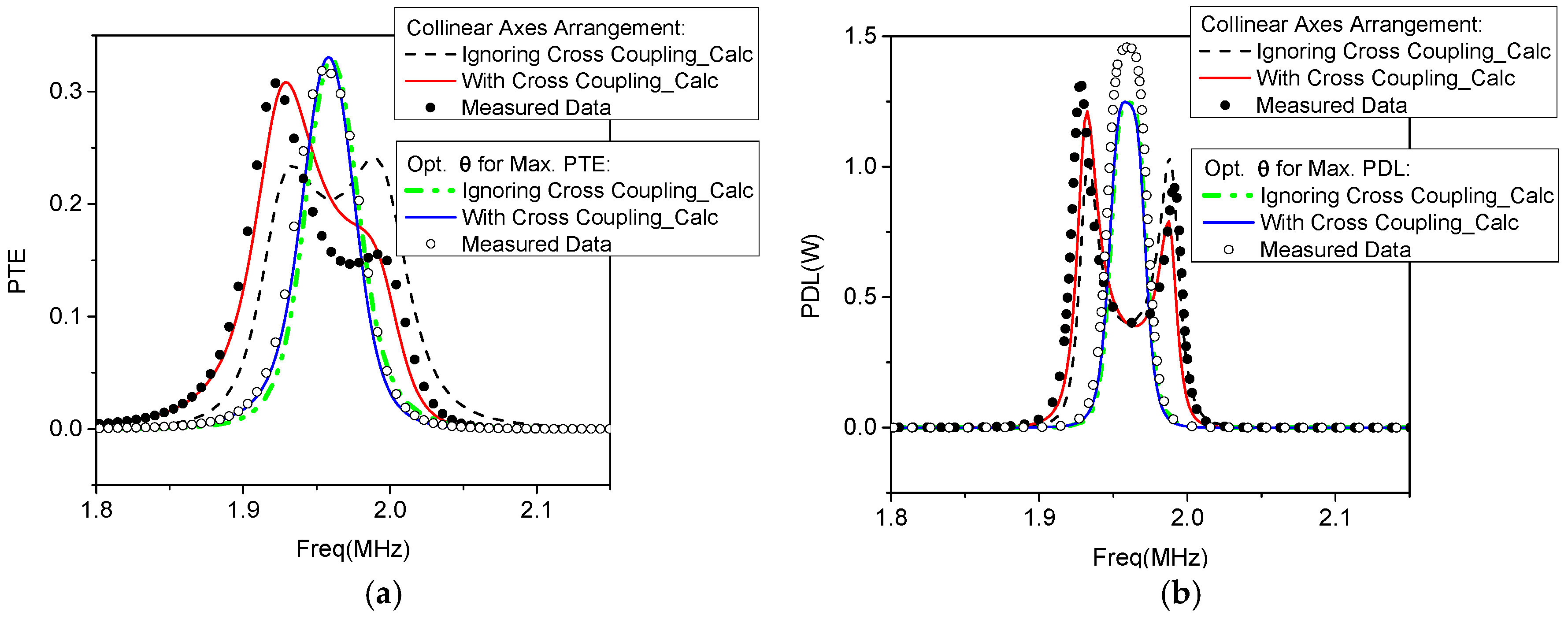
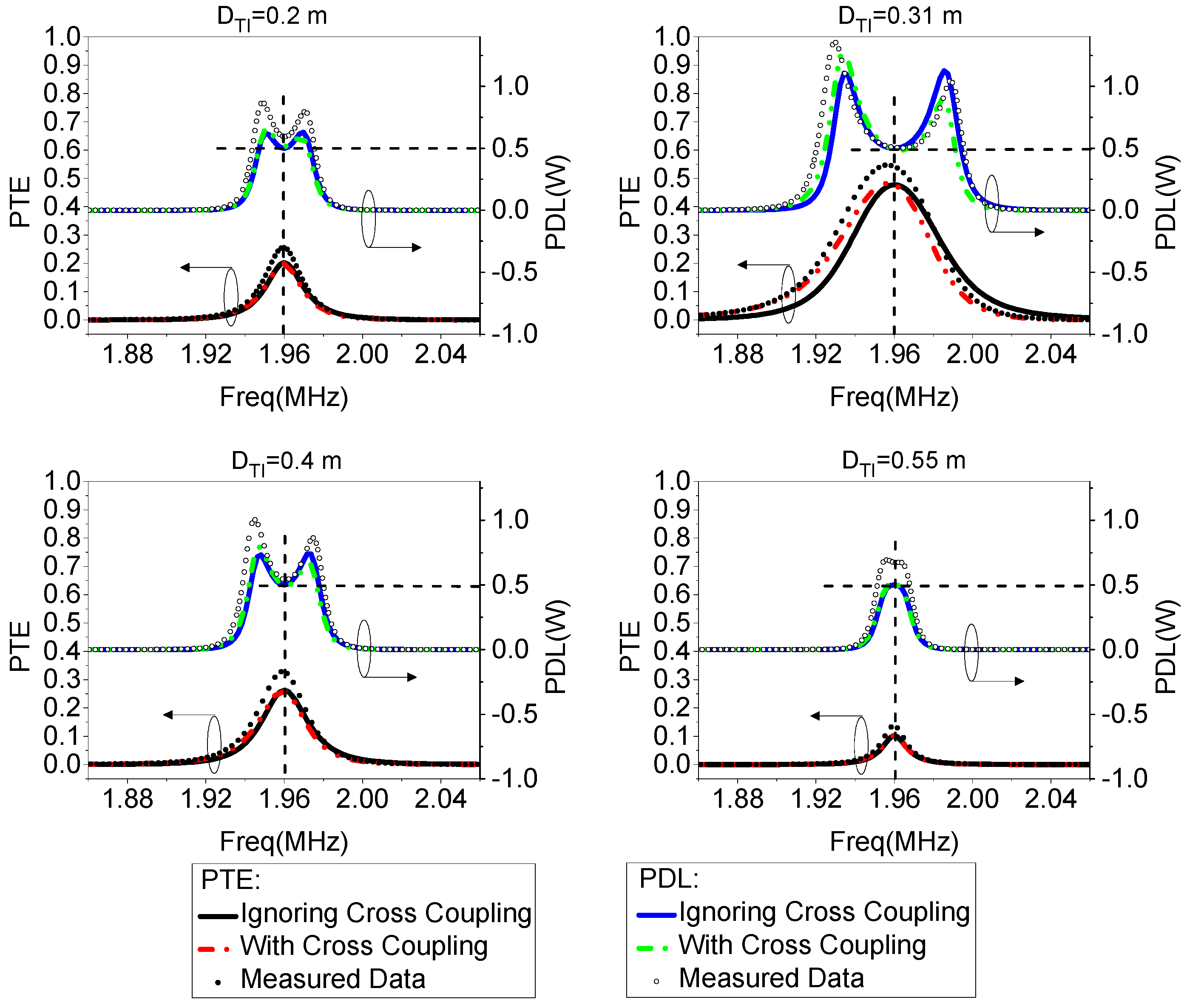
4.2.2. Verification of the Feasibility for Predetermined-Goals Wireless Power Transfer in Three-Resonator System
5. Conclusions
Acknowledgments
Author Contributions
Conflicts of Interest
References
- Xia, M.; Sonia, A. On the efficiency of far-field wireless power transfer. IEEE Trans. Signal Proc. 2015, 63, 2835–2847. [Google Scholar] [CrossRef]
- Zhang, J.; Cheng, C.H. Investigation of Near-Field Wireless Power Transfer between Two Efficient Electrically Small Planar Antennas. In Proceedings of the 2014 3rd Asia-Pacific Conference on Antennas and Propagation (APCAP), Harbin, China, 26–29 July 2014; pp. 720–723.
- Liu, C.; Hu, A.P.; Nair, N.K.C. Modelling and analysis of a capacitively coupled contactless power transfer system. IET Power Electron. 2011, 4, 808–815. [Google Scholar] [CrossRef]
- Zhen, Z.; Chau, K.T. Homogeneous wireless power transfer for move-and-charge. IEEE Trans. Power Electron. 2015, 30, 6213–6220. [Google Scholar]
- Moorey, C.; Holderbaum, W.; Potter, B. Investigation of high-efficiency wireless power transfer criteria of resonantly-coupled loops and dipoles through analysis of the figure of merit. Energies 2015, 8, 11342–11362. [Google Scholar] [CrossRef]
- Gao, Y.; Farley, K.B.; Tse, Z.T.H. A uniform voltage gain control for alignment robustness in wireless ev charging. Energies 2015, 8, 8355–8370. [Google Scholar] [CrossRef]
- RamRakhyani, A.K.; Lazzi, G. On the design of efficient multi-coil telemetry system for biomedical implants. IEEE Trans. Biomed. Circuits Syst. 2013, 7, 11–23. [Google Scholar] [CrossRef] [PubMed]
- Ahn, D.; Hong, S. A study on magnetic field repeater in wireless power transfer. IEEE Trans. Ind. Electron. 2013, 60, 360–371. [Google Scholar] [CrossRef]
- Zhang, F.; Hackworth, S.A.; Fu, W.; Li, C.; Mao, Z.; Sun, M. Relay effect of wireless power transfer using strongly coupled magnetic resonances. IEEE Trans. Magn. 2011, 47, 1478–1481. [Google Scholar] [CrossRef]
- Zhang, X.; Ho, S.; Fu, W. Quantitative design and analysis of relay resonators in wireless power transfer system. IEEE Trans. Magn. 2012, 48, 4026–4029. [Google Scholar] [CrossRef]
- Kim, J.; Son, H.-C.; Kim, K.-H.; Park, Y.-J. Efficiency analysis of magnetic resonance wireless power transfer with intermediate resonant coil. IEEE Antennas Wirel. Propag. Lett. 2011, 10, 389–392. [Google Scholar] [CrossRef]
- Zhong, W.X.; Zhang, C.; Xun, L.; Hui, S.Y.R. A methodology for making a three-coil wireless power transfer system more energy efficient than a two-coil counterpart for extended transfer distance. IEEE Trans. Power Electron. 2015, 30, 933–942. [Google Scholar] [CrossRef]
- Sun, L.; Tang, H.; Zhang, Y. Determining the frequency for load-independent output current in three-coil wireless power transfer system. Energies 2015, 8, 9719–9730. [Google Scholar] [CrossRef]
- Miyamoto, T.; Komiyama, S.; Mita, H.; Fujimaki, K. Wireless Power Transfer System with a Simple Receiver Coil. In Proceedings of the 2011 IEEE MTT-S International Microwave Workshop Series on Innovative Wireless Power Transmission: Technologies, Systems, and Applications (IMWS), Kyoto, Japan, 12–13 May 2011; pp. 131–134.
- Awai, I.; Ikuta, Y.; Sawahara, Y.; Yangjun, T.; Ishizaki, T. Applicaions of a Novel Disk Repeater. In Proceedings of the 2014 IEEE Wireless Power Transfer Conference (WPTC), Jeju, Korea, 8–9 May 2014; pp. 114–117.
- Kiani, M.; Jow, U.-M.; Ghovanloo, M. Design and optimization of a 3-coil inductive link for efficient wireless power transmission. IEEE Trans. Biomed. Circuits Syst. 2011, 5, 579–591. [Google Scholar] [CrossRef] [PubMed]
- Uei-Ming, J.; Ghovanloo, M. Design and optimization of printed spiral coils for efficient transcutaneous inductive power transmission. IEEE Trans. Biomed. Circuits Syst. 2007, 1, 193–202. [Google Scholar]
- Islam, A.B.; Islam, S.K.; Tulip, F.S. Design and optimization of printed circuit board inductors for wireless power transfer system. Circuits Syst. 2013, 4, 237–244. [Google Scholar] [CrossRef]
- RamRakhyani, A.K.; Mirabbasi, S.; Chiao, M. Design and optimization of resonance-based efficient wireless power delivery systems for biomedical implants. IEEE Trans. Biomed. Circuits Syst. 2011, 5, 48–63. [Google Scholar] [CrossRef] [PubMed]
- Ahn, D.; Hong, S. Wireless power transmission with self-regulated output voltage for biomedical implant. IEEE Trans. Ind. Electron. 2014, 61, 2225–2235. [Google Scholar] [CrossRef]
- Villa, J.L.; Sallan, J.; Sanz Osorio, J.F.; Llombart, A. High-misalignment tolerant compensation topology for ICPT systems. Ind. Electron. 2012, 59, 945–951. [Google Scholar] [CrossRef]
- Zhang, J.; Cheng, C.H. Quantitative investigation into the use of resonant magneto-inductive links for efficient wireless power transfer. IET Microw. Antennas Propag. 2016, 10, 38–44. [Google Scholar] [CrossRef]
- Babic, S.I.; Akyel, C. Calculating mutual inductance between circular coils with inclined axes in air. IEEE Trans. Magn. 2008, 44, 1743–1750. [Google Scholar] [CrossRef]
- Sample, A.P.; Meyer, D.A.; Smith, J.R. Analysis, experimental results, and range adaptation of magnetically coupled resonators for wireless power transfer. IEEE Trans. Ind. Electron. 2011, 58, 544–554. [Google Scholar] [CrossRef]
- Park, J.; Tak, Y.; Kim, Y.; Kim, Y.; Nam, S. Investigation of adaptive matching methods for near-field wireless power transfer. IEEE Trans. Antennas Propag. 2011, 59, 1769–1773. [Google Scholar] [CrossRef]
- Pozar, D.M. Microwave Engineering, 3rd ed.; Wiley & Sons, Inc.: New, York, NY, USA, 2005. [Google Scholar]


| Graph and extrema for f(x), where |  | ||
| Locations of x0 | ① x0 < 0 | ② x0 = 0 | ③ x0 > 0 |
| Local minimum of , in this paper | - | ||
| Coupling region for PTE | Non-frequency splitting region | Critical frequency splitting | Frequency splitting region |
| Number of local maximum for PTE | 1 | - | 2 |
| Graphs and extrema for g(x), where |  |  | |||||
| Scope of Δ | Δ > 0 | Δ = 0 | |||||
| Locations of x1 and x2 | |||||||
| Local minimum of , in this paper | - | - | and | - | |||
| Coupling regions for | Non-frequency splitting region | Critical condition 1 1 | Frequency splitting region | Critical condition 2 2 | Frequency splitting region | Non-frequency splitting region | Critical condition 3 3 |
| Frequency number of local maximum for | 1 | - | 2 | - | 3 | 1 | - |
© 2016 by the authors; licensee MDPI, Basel, Switzerland. This article is an open access article distributed under the terms and conditions of the Creative Commons by Attribution (CC-BY) license (http://creativecommons.org/licenses/by/4.0/).
Share and Cite
Zhang, J.; Cheng, C. Analysis and Optimization of Three-Resonator Wireless Power Transfer System for Predetermined-Goals Wireless Power Transmission. Energies 2016, 9, 274. https://doi.org/10.3390/en9040274
Zhang J, Cheng C. Analysis and Optimization of Three-Resonator Wireless Power Transfer System for Predetermined-Goals Wireless Power Transmission. Energies. 2016; 9(4):274. https://doi.org/10.3390/en9040274
Chicago/Turabian StyleZhang, Jin, and Chonghu Cheng. 2016. "Analysis and Optimization of Three-Resonator Wireless Power Transfer System for Predetermined-Goals Wireless Power Transmission" Energies 9, no. 4: 274. https://doi.org/10.3390/en9040274
APA StyleZhang, J., & Cheng, C. (2016). Analysis and Optimization of Three-Resonator Wireless Power Transfer System for Predetermined-Goals Wireless Power Transmission. Energies, 9(4), 274. https://doi.org/10.3390/en9040274