Simulation of Wind Speed in the Ventilation Tunnel for Surge Tanks in Transient Processes

Abstract

Hydroelectric power plants’ open-type surge tanks may be built in mountains subject to the provision of atmospheric air. Hence, a ventilation tunnel is indispensable. The air flow in the ventilation tunnel is associated with the fluctuation of water-level in the surge tank. There is a great relationship between the wind speed and the safe use and project investment of ventilation tunnels. To obtain the wind speed in a ventilation tunnel for a surge tank during transient processes, this article adopts the one-dimensional numerical simulation method and establishes a mathematical model of a wind speed by assuming the boundary conditions of air discharge for a surge tank. Thereafter, the simulation of wind speed in a ventilation tunnel, for the case of a surge tank during transient processes, is successfully realized. Finally, the effective mechanism of water-level fluctuation in a surge tank and the shape of the ventilation tunnel (including length, sectional area and dip angle) for the wind speed distribution and the change process are discovered. On the basis of comparison between the simulation results of 1D and 3D computational fluid dynamics (CFD), the results indicate that the one-dimensional simulation method as proposed in this article can be used to accurately simulate the wind speed in the ventilation tunnel of a surge tank during transient processes. The wind speed fluctuations can be superimposed by using the low frequency mass wave (i.e., fundamental wave) and the high frequency elastic wave (i.e., harmonic wave). The water-level fluctuation in a surge tank and the sectional area of the ventilation tunnel mainly affect the amplitude of fundamental and harmonic waves. The period of a fundamental wave can be determined from the water-level fluctuations. The length of the ventilation tunnel has an effect on the period and amplitude of harmonic waves, whereas the dip angle influences the amplitude of harmonic waves.

1. Introduction

An open-type surge tank built in a mountain must be connected with the atmosphere air by a ventilation tunnel to realize its functions of ventilation and pressure reduction, as shown in Figure 1. In the transient processes of a hydroelectric power plant (HPP), the load rejection and the load adjustment of units can cause water-level fluctuations in a surge tank, and, thereafter, lead to volume, pressure and f air flow changes the surge tank. As a consequence, the gas in the ventilation tunnel transforms from a static state to an unsteady flow causing high speed wind flows. These high speed wind flows will not only affect the tunnel structure and safe use, but it also affects the project investment for the provision of ventilation tunnel. Hence, it is necessary to carry out a simulation of the wind speed during transient processes to provide a basis for the application and design of ventilation tunnels in the case of surge tanks.

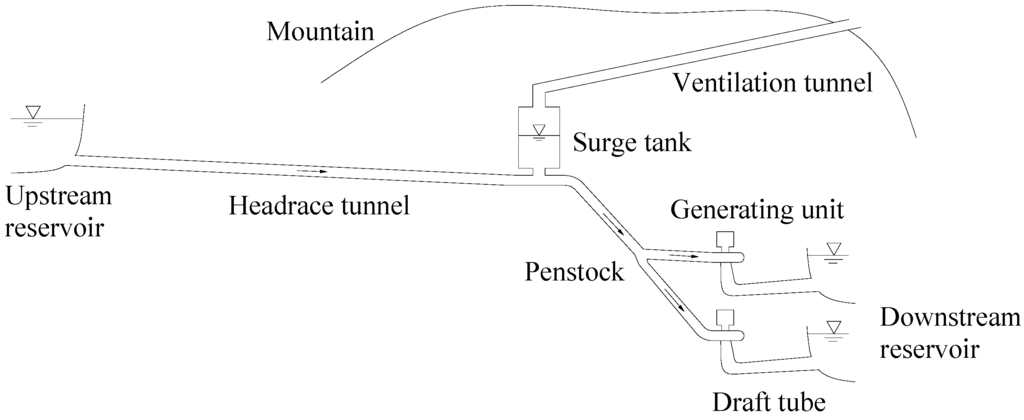
Figure 1. Schematic diagram of the layout of a surge tank and a tunnel in a HPP.

Figure 1. Schematic diagram of the layout of a surge tank and a tunnel in a HPP.

For the case of a wind speed in a tunnel, many measurement methods and simulation techniques have been studied. Davenport [1], Liu et al. [2] and Allegrini et al. [3] have all proposed methods to measure wind speeds in a wind tunnel. Xu [4] made physical models to the ventilation tunnel of a surge tank of an underground HPP. He measured the wind speed and analyzed the relation between the wind speed change process and the water-level fluctuations in a surge tank. Field tests and experiments are important ways to explore the fundamental relationships, but they always demand a great deal of time and money; hence, many researchers prefer to use the numerical simulation technique. Ramponi and Blocken [5] and Mo et al. [6] investigated the wind speed by using the three-dimensional computational fluid dynamics (CFD) method and the effect of turbulence models. Zhou et al. [7] studied the functional mechanism of a ventilation system for the tailrace tunnel by using CFD. The three-dimensional computational method is an accurate tool, but it is also time-consuming. On the other hand, the one-dimensional numerical simulation of wind speed in a ventilation tunnel, for the case of a surge tank during transient processes, has not been investigated. Streeter and Wylie discussed the transient flow in a natural gas pipeline and established its basic equations. In this regard, they proposed to use the one-dimensional method of characteristics (MOC) [8], but the research object they studied is considerably different from a ventilation tunnel and its results cannot be referenced directly. In addition, the boundary conditions of the ventilation tunnel for a surge tank are entirely new problems.

To determine the wind speed in the ventilation tunnel for the case of a surge tank during transient processes, this article uses the one-dimensional numerical simulation method and establishes a mathematical model of wind speed based on the boundary conditions of air discharge for the case of a surge tank. Thereafter, the simulation of wind speed in the ventilation tunnel for a surge tank during transient processes, is successfully realized. By comparing the results of one-dimensional simulation to that of three-dimensional CFD simulation through a project case, the applicability and the rationality of one-dimensional numerical simulation as proposed in this article have been verified. Finally, the effective mechanism of water-level fluctuation in a surge tank and the shape of the ventilation tunnel (including length, sectional area and dip angle) for onward distribution and the wind speed change process have been explored from the perspective of wave superposition.

2. Mathematical Model

The simulation of wind speed in the ventilation tunnel deals with the transient flow of a gas pipeline. The mathematical model established in this section is based on the following assumptions: (1) the flow is isothermal; (2) the elasticity of the pipe’s wall can be ignored; (3) the flow is one dimensional; (4) the coefficient of friction is a function of the surface’s roughness and Reynolds number (when we calculate the transient flow, the steady flow friction coefficient can be used); and (5) any kinetic energy changes along the pipeline can be ignored.

2.1. Basic Equations and Solution of MOC

For the case of unsteady flow of pressurized pipeline, the basic equations include the momentum equation and the continuity equation; their expressions can be written as follows [8]:

$$\text{Continuity equation:} \frac{B^2}{A}\frac{\partial M}{\partial x}+\frac{\partial p}{\partial t}=0$$

(1)

$$\text{Momentum equation:} \frac{\partial p}{\partial x}+\frac{{\mathsf{\alpha }}^2}{A}\frac{\partial M}{\partial t}+\frac{pg\sin \mathsf{\theta }}{B^2}+\frac{f{B}^{2}M\left|M\right|}{2D{A}^{2}p}=0$$

(2)

where the relevant parameters are defined as follows: B = wave velocity; A = sectional area of the ventilation tunnel; M = mass flow; x = position along the axis of the tunnel; p = absolute pressure of gas; t = time; α = inertia factor; g = gravitational acceleration; θ = included angle between the axis of pipeline and the horizontal plane; f = Darcy-Weisbach coefficient of friction resistance; D = diameter of the ventilation tunnel.

It should be noted that:

(1)

$M=\mathsf{\rho }vA$, where v = flow velocity.

(2)

The wave velocity can be determined by using the state equation $B=\sqrt{p/\mathsf{\rho }}=\sqrt{\mathsf{\lambda }RT}$; where $\mathsf{\rho }$ is the gas density, λ is the compressibility coefficient, R is the gas constant and T is the absolute temperature.

(3)

When the axis rises up along the direction of +x, θ, the included angle between the axis of pipeline and the horizontal plane, takes a positive value.

(4)

The default values of the parameters are: B = 340 m/s, α = 1, f = 0.015, $\mathsf{\rho }$ = 1.205 kg/m³, p₀ = 101,325 Pa.

The MOC grid is shown in Figure 2. The equations of positive and negative characteristics along with the positive characteristic line $\frac{\mathrm{d}x}{\mathrm{d}t}=\frac{B}{\mathsf{\alpha }}$ and the negative characteristic line $\frac{\mathrm{d}x}{\mathrm{d}t}=-\frac{B}{\mathsf{\alpha }}$ can be obtained as follows (expressed by $C^{+}$ and $C^{-}$, respectively):

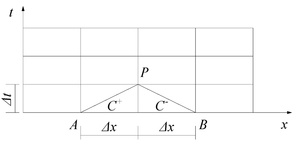
Figure 2. The characteristic grids and characteristic lines.

Figure 2. The characteristic grids and characteristic lines.

$$C^{+}\{\begin{array}{l}\frac{{\mathsf{\alpha }}^2}{A}\frac{\mathrm{d}M}{\mathrm{d}t}+\frac{\mathsf{\alpha }}{B}\frac{\mathrm{d}p}{\mathrm{d}t}+\frac{pg\sin \mathsf{\theta }}{B^2}+\frac{f{B}^{2}M\left|M\right|}{2D{A}^{2}p}=0\\ \frac{\mathrm{d}x}{\mathrm{d}t}=\frac{B}{\mathsf{\alpha }}\end{array}$$

(3)

$$C^{-}\{\begin{array}{l}\frac{{\mathsf{\alpha }}^2}{A}\frac{\mathrm{d}M}{\mathrm{d}t}-\frac{\mathsf{\alpha }}{B}\frac{\mathrm{d}p}{\mathrm{d}t}+\frac{pg\sin \mathsf{\theta }}{B^2}+\frac{f{B}^{2}M\left|M\right|}{2D{A}^{2}p}=0\\ \frac{\mathrm{d}x}{\mathrm{d}t}=-\frac{B}{\mathsf{\alpha }}\end{array}$$

(4)

By using the integrated method along the characteristic lines ($C^{+}:A\to P$, $C^{-}:B\to P$), we can get equations for $C^{+}$ and $C^{-}$:

$$C^{+}:p_P=C_P-C_B{M}_P$$

(5)

$$C^{-}:p_P=C_M+C_B{M}_P$$

(6)

Thereafter, the intensity of pressure and the mass flow at the point P can be expressed as follows:

$$p_P=\frac{C_P+C_M}{2}$$

(7)

$$M_P=\frac{C_P-C_M}{2C_B}$$

(8)

where, $C_P=p_A+\frac{\mathsf{\alpha }B}{A}{M}_A-(\frac{p_{A}g\sin \mathsf{\theta }}{\mathsf{\alpha }B}+\frac{f{B}^3{M}_A\left|M_A\right|}{2\mathsf{\alpha }D{A}^2{p}_A})\Delta t$, $C_M=p_B-\frac{\mathsf{\alpha }B}{A}{M}_B-(\frac{p_{B}g\sin \mathsf{\theta }}{\mathsf{\alpha }B}+\frac{f{B}^3{M}_B\left|M_B\right|}{2\mathsf{\alpha }D{A}^2{p}_B})\Delta t$, $C_B=\frac{\mathsf{\alpha }B}{A}$.

2.2. Boundary Conditions and Initial Conditions

2.2.1. Boundary Conditions

The boundary conditions for the “surge tank—ventilation tunnel” system, as shown in Figure 3, includes the last section of the ventilation tunnel (i.e., the atmospheric air side), the connecting pipes and the first section of the ventilation tunnel (i.e., the surge tank side). It should be noticed that the first section and the last section of ventilation tunnel can be considered the positive direction of the pipeline as it assumed in this article (i.e., from the surge tank side towards the atmospheric air side). These boundary conditions have been discussed as follows:

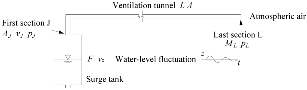
Figure 3. The boundary conditions of the first section of a ventilation tunnel.

Figure 3. The boundary conditions of the first section of a ventilation tunnel.

(1)

Last section of the ventilation tunnel (i.e., the atmospheric air side)

The last section of the ventilation tunnel is directly connected to the atmosphere. Its pressure is identical to the atmospheric pressure, i.e., p_L = p₀. By using the $C^{-}$ equation, the unknown quantity M_L of this boundary node can be obtained as follows:

$$M_L=\frac{p_0-C_M}{C_B}$$

(9)

(2)

Connecting pipes

The junctions of pipes in a series (refer to Figure 4) meet the continuous mass flow condition. Meanwhile, the pressure of the sections just before and after the junction should be treated the same, if the local loss of head is neglected. By using the $C^{+}$ and $C^{-}$ equations, we can get the boundary conditions of pipes in a series as follows:

$$p_P=\frac{C_{B1}{C}_{M2}+C_{B2}{C}_{P1}}{C_{B1}+C_{B2}}$$

(10)

$$M_P=\frac{C_{P1}-C_{M2}}{C_{B1}+C_{B2}}$$

(11)

Figure 4. The boundary condition of pipes in a series.

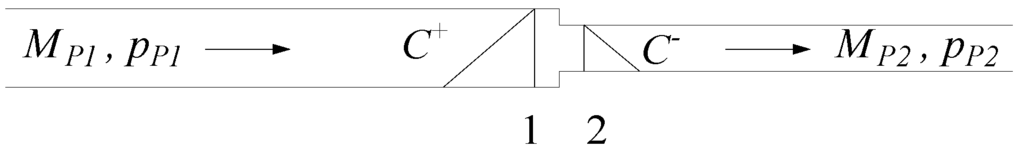
Figure 4. The boundary condition of pipes in a series.

(3)

First section of the ventilation tunnel (i.e., the surge tank side)

The water-level fluctuation of a surge tank serves as a source of disturbances. This leads to the unsteady flow of the air in a surge tank and in a ventilation tunnel. In this article, we allow the fluctuation of the water-level in a surge tank to be known, i.e., z = z(t). The fluctuation process in the water-level of a surge tank can be simulated by using software for the transient processes of a HPP and by neglecting the air dynamics in the ventilation tunnel. Next, it is assumed that the initial water level is zero and the upward movement can be treated as positive.

It is presumed that the velocity of fluctuation in the water-level for the case of a surge tank (v_z) and the flow rate of gas (v_J) at the first section of the ventilation tunnel should meet the following relationship:

$$v_{z}F=v_J{A}_J$$

(12)

where, F is the sectional area of a surge tank; A_J is the sectional area of the first section of the ventilation tunnel.

By substituting the $v_z=-\frac{\mathrm{d}z}{\mathrm{d}t}$ and $M_J=\mathsf{\rho }{v}_J{A}_J$ in Equation (12) and by simplifying the resulting equation, we may get:

$$M_J=-\mathsf{\rho }F\frac{\mathrm{d}z}{\mathrm{d}t}$$

(13)

By applying the $C^{+}$ equation, the unknown quantity $p_J$ at the boundary node can be obtained as follows:

$$p_J=C_P-C_B{M}_J$$

(14)

It should be noticed that there might be some other treatment methods for the boundary conditions of the first section of a ventilation tunnel. The treatment method, as adopted in this article, can be used to reflect the dynamic nature and the characteristics of air flow in the ventilation tunnel.

2.2.2. Initial Conditions

For the case of an isothermal (steady) flow, $M$ is the constant and $\frac{\partial M}{\partial t}=0$. The integral of momentum equation from $x=0$ at $p=p_1$ to $x=\Delta x$ at $p=p_2$ yields:

$$p_2^2=(p_1^2-\frac{f{B}^{2}M\left|M\right|}{D{A}^2}\Delta x\frac{e^s-1}{s})/e^s$$

(15)

In Equation (15): $s=(2g\Delta x\sin \theta )/B^2$. This equation presents the parabolic pressure gradient of the ventilation tunnel in a steady state. The pressure at every section of the ventilation tunnel during the initial steady state should satisfy this equation. For the case of a horizontal pipeline, $s=0$, $e^s=1$ and $(e^s-1)/s=1$, therefore, Equation (15) becomes:

$$p_2^2=p_1^2-\frac{f{B}^{2}M\left|M\right|}{D{A}^2}\Delta x$$

(16)

If the air in the pipeline is static in the initial state, then the flow at every section is equal to zero. As a consequence, the pressure at every section in the pipeline is always equal to the atmospheric pressure.

3. Solution and Model Verification

3.1. The Solution

In accordance with the mathematical model developed in Section 2, the simulation of wind speed in the ventilation tunnel for the case of a surge tank during transient processes can be carried out. The steps involved in the computational procedure, are as follows: (1) divide the pipeline of the ventilation tunnel into several sections. The space steps and the time steps can be denoted as $\Delta x$ and $\Delta t$, respectively where $\Delta x=(B/\mathsf{\alpha })/\Delta t$. On the basis of the initial condition at time $t=t_0$, the $C_P$, $C_M$ and $C_B$ can be determined, thereafter, $p_P$ and $M_P$ at the time $t=t_0+\Delta t$ can be determined by using Equations (7) and (8). When the boundary nodes located in the last section of the ventilation tunnel, the pipes in a series and the first section of a ventilation tunnel must be computed, the boundary conditions discussed in Section 2.2.1 should be applied. We follow the above-described procedure for the total calculation time set in advance. The complete simulation process is shown in Figure 5.

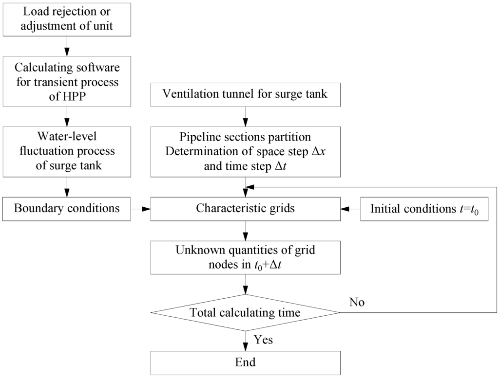
Figure 5. The complete simulation process of the wind speed in the ventilation tunnel for the case of a surge tank during a transient process.

Figure 5. The complete simulation process of the wind speed in the ventilation tunnel for the case of a surge tank during a transient process.

3.2. Model Verification

To verify the correctness of the one-dimensional simulation for the case of wind speed in a ventilation tunnel, as proposed in this article, a project case is selected for a comparison between the simulation results of the one-dimensional method and that of a three-dimensional CFD method. The layout for the “surge tank—ventilation tunnel” system and the process of water-level fluctuation for the case of a surge tank are shown in Figure 6. The basic parameters are defined as follows: for the ventilation tunnel: the vertical pipeline is L_JB = 85 m, the horizontal pipeline is L_BL = 680 m, the sectional area A = 20 m²; for the surge tank case, the sectional area is F = 706.86 m².

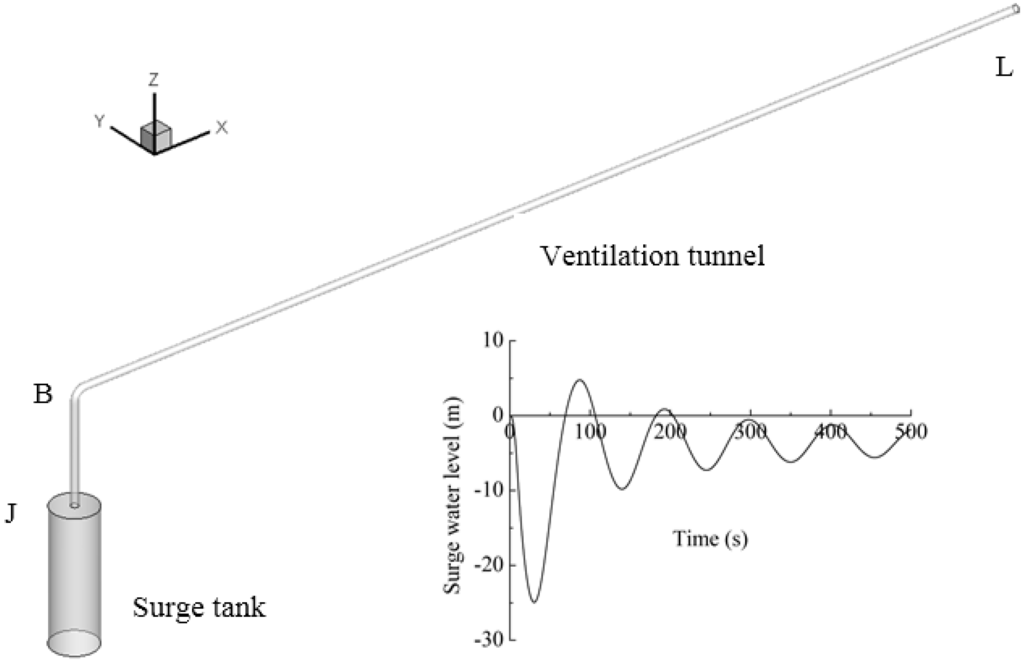
Figure 6. The layout for the “surge tank—ventilation tunnel” system and the water-level fluctuation process for the case of a surge tank (project case).

Figure 6. The layout for the “surge tank—ventilation tunnel” system and the water-level fluctuation process for the case of a surge tank (project case).

The assessment region of the one-dimensional method is between the first section (i.e., Section J, the connecting section between the ventilation tunnel and the surge tank) and the last section (i.e., Section L, the ventilation tunnel exit that is connected to the atmosphere). The three-dimensional CFD method conducts the assessment from the free water surface of a surge tank to Section L. In the three-dimensional CFD simulation case, the volume of fluid (VOF) multiphase flow model [9,10], the second order realizable k-ε turbulence model [11], the standard near wall function [12], the incompressible Navier-Stokes (NS) equation dispersed by the finite volume method (FVM) [13] and pressure implicit with splitting of operator (PISO) algorithm, that are coupled by pressure and velocity [14,15,16,17], are adopted. The boundary conditions of a surge tank are adopted for the preset water-level fluctuation process, as shown in Figure 6, whereas the boundary conditions of Section L are fixed to use the preset atmospheric pressure (p₀). The results for the distribution of wind speed (i.e., the positive and negative extremum envelope curves along the axis of ventilation tunnel) and the fluctuation processes of wind speed at typical sections (i.e., Section J, Section L and the Section B) simulated by using these two methods are compared and shown in Figure 7 and Figure 8). Please notice that: (1) the positive wind speed flows from Section J towards Section L, whereas the inverse flow is negative; (2) the axis length is calculated between Section J and Section L.

Figure 7 and Figure 8 show that: (1) according to the 3D method, the absolute values of positive and negative wind speed extrema along the axis of ventilation tunnel present an almost linear and gradually increasing tendency. The amplification of the positive extremum is small while the amplification of the negative extremum is large (refer to Table 1). Hence, the maximum values of positive and negative wind speed occur at Section L. For the 1D method, the distribution trend of wind speed (extremum) is the same as that of the 3D method. The positive extreme values at Sections J and L are respectively higher and lower than those estimated by the 3D method, whereas the absolute values of negative wind speed (extremum) are always higher than those of the 3D method. In the same section, there is an insignificantly small difference of wind extreme values between the 1D and 3D methods (the positive difference is less than 1.42 m/s and 4.86%, the negative difference is less than 5.76 m/s and 8.69%).

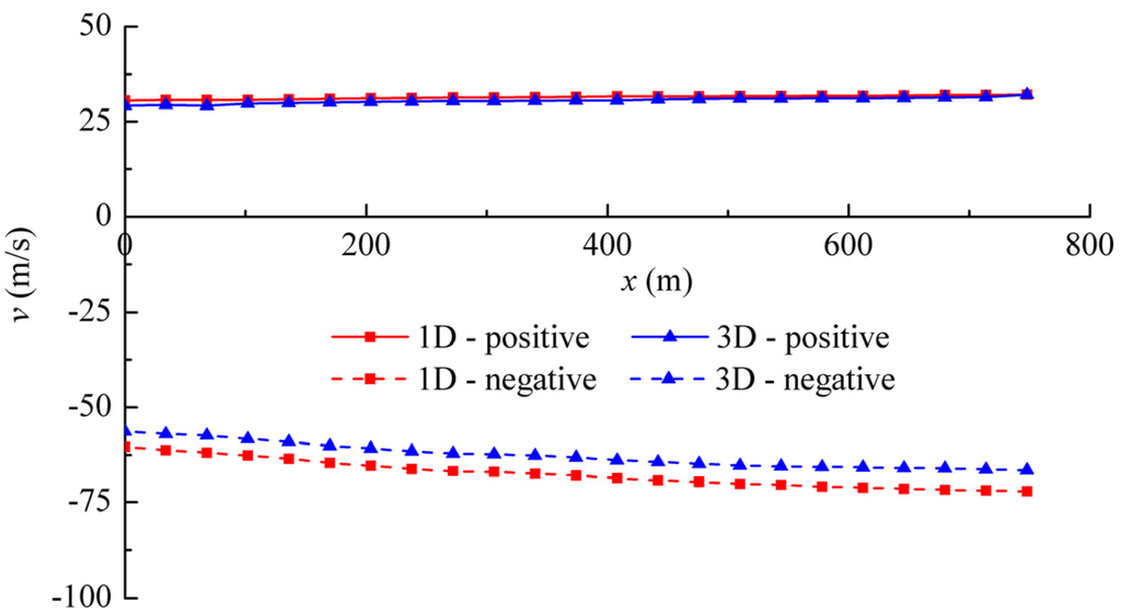
Figure 7. The comparison of the positive and negative (extremum) envelope curves along the axis of ventilation tunnel, simulated by 1D and 3D methods.

Figure 7. The comparison of the positive and negative (extremum) envelope curves along the axis of ventilation tunnel, simulated by 1D and 3D methods.

Figure 8. The comparison of the wind speed fluctuation processes of typical sections as simulated by using 1D and 3D methods.

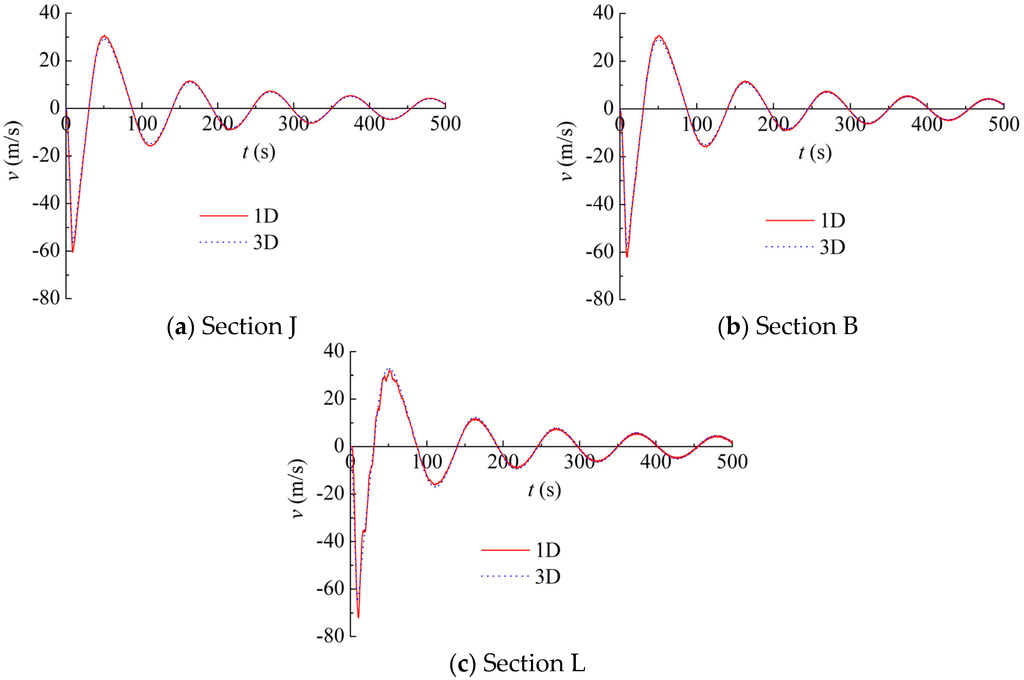
Figure 8. The comparison of the wind speed fluctuation processes of typical sections as simulated by using 1D and 3D methods.

Table 1. The comparison of positive and negative wind speeds (extrema) in typical sections.

Simulation Method	Positive Wind Speed Extrema (m/s)			Negative Wind Speed Extrema (m/s)
	Section J	Section B	Section L	Section J	Section B	Section L
Three-dimensional CFD (3D)	29.21	29.24	32.82	−56.42	−57.42	−65.88
One-dimensional (1D)	30.63	30.70	32.09	−60.51	−62.42	−72.15

Table 1. The comparison of positive and negative wind speeds (extrema) in typical sections.

Simulation Method	Positive Wind Speed Extrema (m/s)			Negative Wind Speed Extrema (m/s)
	Section J	Section B	Section L	Section J	Section B	Section L
Three-dimensional CFD (3D)	29.21	29.24	32.82	−56.42	−57.42	−65.88
One-dimensional (1D)	30.63	30.70	32.09	−60.51	−62.42	−72.15

(2) In the same section, the processes involved in wind fluctuation (including period, amplitude, attenuation rate, initial phase, etc.) in the 1D and 3D methods do not differ and their fluctuation curves almost coincide with each other. The fluctuation of wind speed has similar rules, when we compare it with the water-level fluctuation of a surge tank. With the attenuated fluctuation of the water-level in a surge tank around its steady value, the wind speed fluctuates gradually around zero. These results indicate that the wind speed depends on the speed of fluctuation of the water-level. The negative and positive wind speeds (extrema) occur at the time of the fastest water-level drop and fastest rise, respectively. For this calculation case, because the fastest water-level decrease speed is greater than the fastest increase speed, the absolute value of the negative wind speed extremum is greater than that of the positive extremum in the same section.

(3) With regard to the gas compressibility, Figure 9 shows the gas pressure change process of Section J that is simulated by using the 1D method. It can be found that the gas pressure has a slight fluctuation, which only influences the gas density, hence, the gas compressibility in the ventilation tunnel can be ignored. For the conditions of general load adjustment of the unit, the range of load changes is small, so the above result can always be applied.

On the basis of the above analysis, the 1D simulation method, as proposed in this article, can accurately simulate the wind speed in the ventilation tunnel of a surge tank during the transient process.

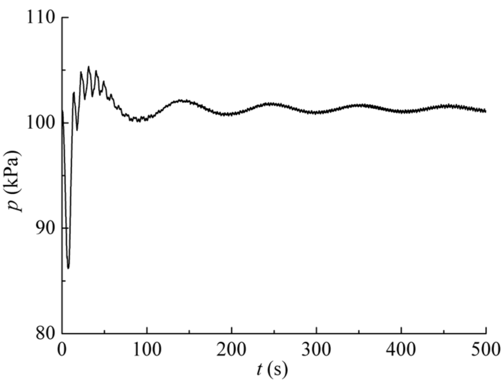
Figure 9. The gas pressure change process of Section J, as simulated by the 1D method.

Figure 9. The gas pressure change process of Section J, as simulated by the 1D method.

4. Analysis of the Influencing Factors’ Effect on Wind Speed

For the “surge tank—ventilation tunnel” system the wind speed of the ventilation tunnel results from the water-level fluctuation in the surge tank, which mainly depends on the operating conditions of the transient process (i.e., load rejection, load increase, etc. [18,19,20,21,22,23]). Next, there is a certain influence of the shape of ventilation tunnel (including length, sectional area and dip angle) on the wind speed distribution and change process. In this section, the effects of above referred (two) kinds of influencing factors on the wind speed are analyzed by using the 1D method, as proposed in the sections above. The basic parameters of the ventilation tunnel are as follows: horizontal arrangement, L = 500 m, A = 20 m², F = 500 m², θ = 0°.

4.1. Effect of the Water-Level Fluctuation Process in a Surge Tank

The four typical operating conditions of unit load adjustment [18,19,20,21,22,23], i.e., load rejection (LR), load increase (LI), load first rejection and then increase (LRI), and load first increase and then rejection (LIR), are selected. Under these four operating conditions, the water-level fluctuation processes in a surge tank are shown in Figure 10a. The simulation results of the positive and negative (extremum) envelope curves along the ventilation tunnel axis and the wind speed fluctuation processes of typical sections (i.e., the first section and the last section) are shown in Figure 10b–d. Figure 10 shows that:

(1) For the case of (extremum) envelope curves, the absolute positive and negative wind speed (extremum) values along the ventilation tunnel axis present a gradually increasing linear tendency, whereas the maximum positive and negative wind speed values occur in the last section. For the maximum positive wind speed values, the values of LIR and LI are high and low, respectively, whereas the values of LR and LRI are the same. For the maximum negative wind speed values, the values of LRI and LR are high and low, respectively, whereas the values of LI and LIR are the same. The plausible cause of the above-described results is that the water-level fluctuation curves between LR and LRI as well as between LI and LIR coincide with each other during the initial period, when the positive and negative wind speed extrema occur.

Figure 10. Effect on the processes of the water-level fluctuation in a surge tank due to the wind speed of ventilation tunnel. (a) The processes of water-level fluctuation of a surge tank under four typical operating conditions; (b) The positive and negative (extremum) envelope curves along the axis of ventilation tunnel; (c) The fluctuation processes of wind speed at the first section; (d) The fluctuation processes of wind speed at the last section.

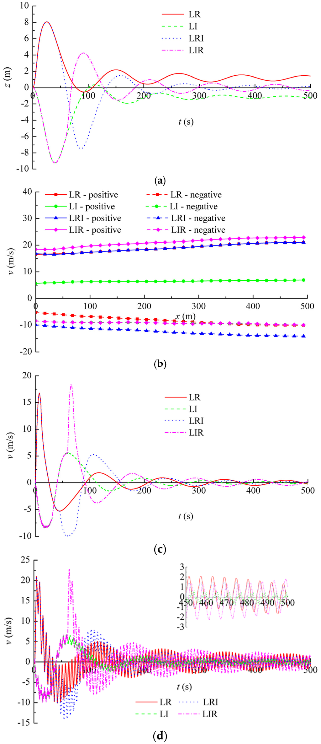
Figure 10. Effect on the processes of the water-level fluctuation in a surge tank due to the wind speed of ventilation tunnel. (a) The processes of water-level fluctuation of a surge tank under four typical operating conditions; (b) The positive and negative (extremum) envelope curves along the axis of ventilation tunnel; (c) The fluctuation processes of wind speed at the first section; (d) The fluctuation processes of wind speed at the last section.

(2) By comparing the wind fluctuation processes of the first and last section, the first section presents smooth curves, whereas the last section shows an apparent fluctuation (i.e., superposition phenomenon). For the superposition case of the last section, the low frequency sub-wave is treated as the fundamental wave, which can be derived by using the water-level fluctuation in the surge tank and has the same fluctuation process as the first section. The high frequency sub-wave is the harmonic wave that can be derived by using the gas elasticity. In this case, the harmonic wave is the flowing gas wave reflected by atmospheric air into the outlet. The fundamental wave corresponds to the mass wave and its period is equal to the period of the water-level fluctuation in the surge tank, whereas its amplitude is influenced by both the fluctuation speed and water-level and the mass flow in the ventilation tunnel. The harmonic wave corresponds to the elasticity wave; its period (4L/B) is proportional to the length and its amplitude is proportional to the gas inertia in the ventilation tunnel. The amplitude of the harmonic wave increases gradually along the axis from the first section (i.e., in the first section it is zero) towards the last section and decreases gradually over time.

4.2. Effect of the Shape of Ventilation Tunnel

4.2.1. Length of Ventilation Tunnel

For different ventilation tunnel lengths (i.e., L = 100, 300, 500, 700 and 900 m), the simulation results of the positive and negative (extrema) envelope curves along the axis and the wind speed fluctuation processes of typical sections (i.e., the first section and the last section) are shown in Figure 11. Figure 11 shows that:

(1) For the cases of different ventilation tunnel lengths, the positive (or negative) wind speed (extreme) in the first section is the same, and the fluctuation process curves coincide with each other. The absolute values of the positive and negative wind speed (extrema) along the axis of the ventilation tunnel present a gradually increasing linear tendency. As the length increases, the absolute values of the positive and negative wind speed (extrema) in the last section tend to rise.

Figure 11. Effect of the length of ventilation tunnel on wind speed; (a) Positive and negative (extrema) envelope curves along the ventilation tunnel axis; (b) wind speed fluctuation processes in the first section; (c) wind speed fluctuation processes in the last section.

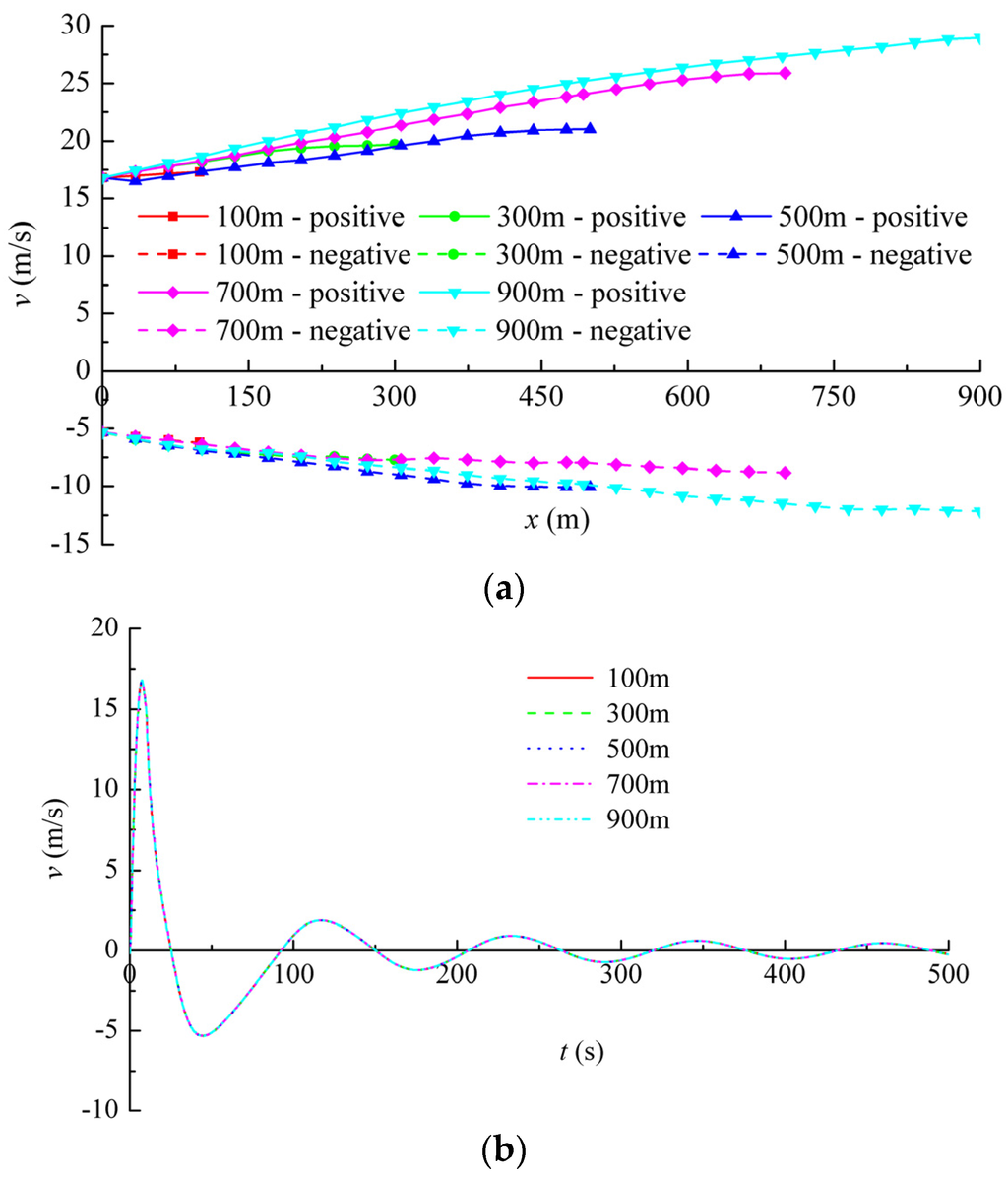
Figure 11. Effect of the length of ventilation tunnel on wind speed; (a) Positive and negative (extrema) envelope curves along the ventilation tunnel axis; (b) wind speed fluctuation processes in the first section; (c) wind speed fluctuation processes in the last section.

(2) As the length increases, the fundamental waves of the wind speed in different sections remain unchanged because the mass flows in different sections remain the same; the amplitude and period (4L/B) of the harmonic wave increase remarkably (because the longer the length, the larger the gas inertia in the ventilation tunnel). The superposition of the fundamental wave and of harmonic waves leads to the rising absolute values of the wind speed (extrema) in the same section.

4.2.2. Sectional Area of Ventilation Tunnel

For the case of different ventilation tunnel sectional areas (i.e., A = 10, 15, 20, 25 and 30 m²), the simulation results of the positive and negative (extrema) envelope curves along the axis as well as the wind speed fluctuation processes in typical sections (i.e., the first section and the last section) have are shown in Figure 12.

Figure 12. Effect of the ventilation tunnel sectional area on wind speed. (a) Positive and negative (extrema) envelope curves along the ventilation tunnel axis; (b) wind speed fluctuation processes in the first section; (c) wind speed fluctuation processes in the last section.

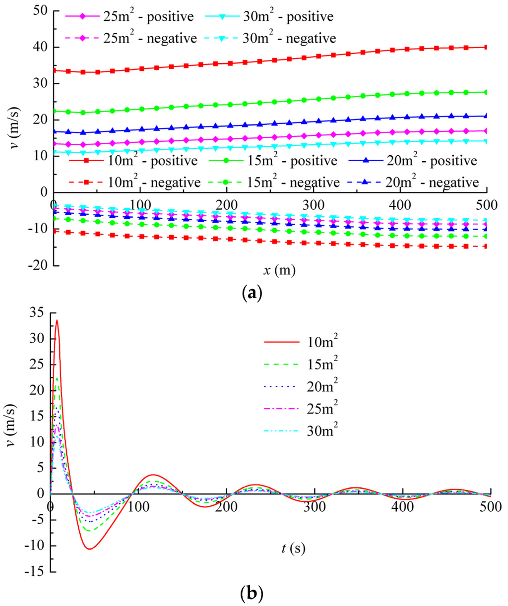
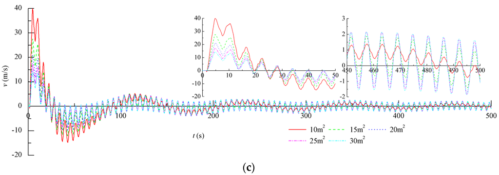
Figure 12. Effect of the ventilation tunnel sectional area on wind speed. (a) Positive and negative (extrema) envelope curves along the ventilation tunnel axis; (b) wind speed fluctuation processes in the first section; (c) wind speed fluctuation processes in the last section.

Figure 12 shows that as the sectional area increases, the period of the fundamental wind speed fluctuation wave in the same section remains unchanged, whereas the amplitude gradually decreases. The period of the harmonic wave in the same section remains unchanged, whereas its amplitude increases gradually due to the rising inertia as the sectional area increases. Since the decrease of the amplitude of fundamental wave plays a leading role, the absolute wind speed (extrema) values in the same section are reduced as the sectional area increases when we consider the superposition of the fundamental and harmonic waves.

4.2.3. Dip Angle of Ventilation Tunnel

For different cases of ventilation tunnel dip angles (i.e., θ = 0°, 10°, 20°, 30°, 40°, 90°), the simulation results of the positive and negative (extrema) envelope curves along the axis and the wind speed fluctuation processes in typical sections (i.e., the first section and the last section) are shown in Figure 13.

Figure 13. Effect of the ventilation tunnel dip angles on wind speed. (a) Positive and negative (extrema) envelope curves along the ventilation tunnel axis; (b) wind speed fluctuation processes in the first section; (c) wind speed fluctuation processes in the last section.

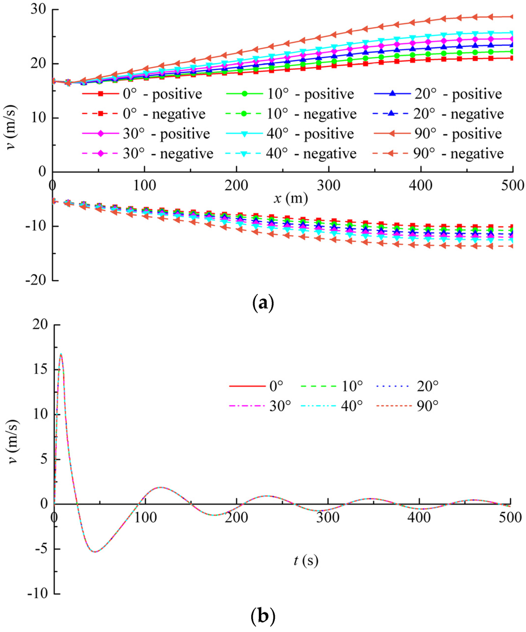
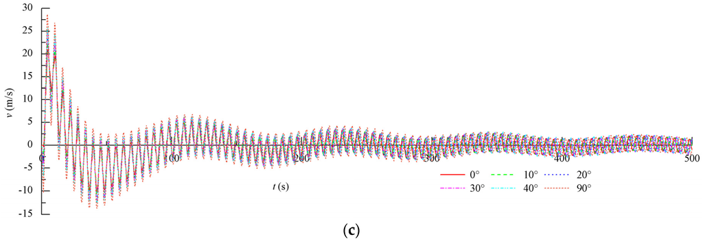
Figure 13. Effect of the ventilation tunnel dip angles on wind speed. (a) Positive and negative (extrema) envelope curves along the ventilation tunnel axis; (b) wind speed fluctuation processes in the first section; (c) wind speed fluctuation processes in the last section.

From the inspection of Figure 13, we can infer that the dip angle effect is similar to that of length as described hereunder:

(1) For different cases of ventilation tunnel dip angle, the positive (or negative) wind speed (extrema) in the first section are the same and the fluctuation process curves coincide with each other. The absolute values of the positive and negative wind speed (extrema) along the ventilation tunnel axis present a gradually increasing linear tendency. As the dip angles increase, the absolute values of the positive and negative wind speed (extrema) in the last section tend to rise.

(2) As the dip angle increases, the fundamental wind speed waves and the period of the harmonic waves in different sections remain unchanged; the harmonic wave amplitude increases because the gas inertia in the direction is augmented by the weight component of the gas when the dip angle rises. The superposition of fundamental and harmonic waves leads to the rise in the absolute wind speed values (extrema) at the same section.

4.3. Summary for the Influencing Factors Effect Analysis

From the perspective of wave superposition theory, Section 4.1 and Section 4.2 reveal the effective mechanism of water-level fluctuation in a surge tank as well as the shape of ventilation tunnel (including length, sectional area and dip angle) for onward distribution and wind speed change processes in a surge tank ventilation tunnel. The water-level fluctuation in the surge tank as well as the sectional area of the ventilation tunnel mainly affect the amplitude of the fundamental and harmonic waves. The period of the fundamental wave can be determined by using the water-level fluctuation. The length of the ventilation tunnel can greatly affect the period and amplitude of harmonic waves, whereas the dip angle influences the harmonic wave amplitude.

On the basis of the results described above, we can devise some appropriate measures that can be adopted for practical purposes to reduce the harm of high speed of wind in a ventilation tunnel. The optimization, regarding the type of load adjustment as well as the increase of sectional area for a ventilation tunnel, is the most effective way to reduce the wind speed.

5. Conclusions

The aim of this article was to adopt a 1D numerical simulation method to establish the mathematical model of “surge tank—ventilation tunnel” system and to derive a wind speed simulation method. Thereafter, from the perspective of wave superposition, the effective mechanism of water-level fluctuations in a surge tank and the shape of the ventilation tunnel for onward distribution and the wind speed change processes are discovered. The major conclusions can be summarized as follows:

(1) The one-dimensional simulation method, as proposed in this article, can be used to accurately simulate the wind speed in the ventilation tunnel of a surge tank during transient processes.

(2) The fluctuation in wind speed can be superimposed by using the low frequency fundamental waves as well as the high frequency harmonic waves. The fundamental waves can be derived by using the water-level fluctuation in a surge tank. It has the same fluctuation process to that of the first section, whereas the harmonic waves can be derived by using the gas elasticity and correspond to the reflected wave of flowing gas by atmospheric air entering the outlet. The fundamental wave corresponds to the mass wave; its period is equal to the period of the water-level fluctuation in a surge tank and its amplitude is influenced by the water-level fluctuation speed and the mass flow in the ventilation tunnel. The harmonic wave corresponds to the elasticity wave; its period (4L/B) is proportional to the length and its amplitude is proportional to the gas inertia in the ventilation tunnel. The amplitude of a harmonic wave increases gradually from the first section (i.e., the first section is zero) to the last section along the axis and gradually decreases over time.

(3) The water-level fluctuation in a surge tank and the sectional area of the ventilation tunnel greatly affect the amplitude of the fundamental and harmonic waves. The period of a fundamental wave can be determined by using the water-level fluctuation. The ventilation tunnel length can be used to greatly affect the period and amplitude of harmonic waves, whereas the dip angle influences the harmonic wave amplitude.

The simulation of wind speed can be used to provide a good reference for ventilation tunnel design purposes. As a result, the hydroelectric power plants can be operated safely and the energy production would become more stable over time.

To summarize, the simulation results of a project case have been compared to the results of prototype measurements, and, their comparison establishes a good agreement. In any future work, we would conduct transient (model) experiments of the wind speed in ventilation tunnels for a surge tank to further validate the simulation method as proposed in this article.

References

- Davenport, A.G. Past, present and future of wind engineering. J. Wind Eng. Ind. Aerodyn. 2002, 90, 1371–1380. [Google Scholar] [CrossRef]
- Liu, Z.J.; Dong, T.T.; Fu, Z. Wind tunnel wind speed control system based on PMAC controller. Mechatronics 2013, 3, 50–54. [Google Scholar]
- Allegrini, J.; Dorer, V.; Carmeliet, J. Wind tunnel measurements of buoyant flows in street canyons. Build. Environ. 2013, 59, 315–326. [Google Scholar] [CrossRef]
- Xu, J.X. Experimental investigation on wind speed of traffic cave in tailwater tunnel. J. Tianjin Univ. 1994, 27, 224–231. [Google Scholar]
- Ramponi, R.; Blocken, B. CFD simulation of cross-ventilation flow for different isolated building configurations: Validation with wind tunnel measurements and analysis of physical and numerical diffusion effects. J. Wind Eng. Ind. Aerodyn. 2012, 104–106, 408–418. [Google Scholar] [CrossRef]
- Mo, J.O.; Choudhry, A.; Arjomandi, M. Effects of wind speed changes on wake instability of a wind turbine in a virtual wind tunnel using large eddy simulation. J. Wind Eng. Ind. Aerodyn. 2013, 117, 38–56. [Google Scholar] [CrossRef]
- Zhou, J.J.; Yang, J.D.; Wang, H. Study on the function mechanism of ventilation system for the tailrace tunnel. Chin. Rural Water Conserv. Hydropower 2012, 7, 171–175. [Google Scholar]
- Streeter, V.L.; Wylie, E.B. Fluid Transients; McGraw-Hill: New York, NY, USA, 1978. [Google Scholar]
- Li, R.; Li, H.; Li, J. Application of gas-liquid two-phase theory for the water surface calculation in open channels. J. Hydrodyn. Ser. A 2002, 17, 77–83. [Google Scholar]
- Ito, K.; Kunugi, T.; Ohshima, H. A high precision unstructured adaptive mesh technique for gas-liquid two-phase flows. Int. J. Numer. Methods Fluids 2011, 67, 1571–1589. [Google Scholar] [CrossRef]
- Wang, J.Y.; Hu, X.J. Application of RNG k-ε turbulence model on numerical simulation in vehicle external flow field. Appl. Mech. Mater. 2012, 170–173, 3324–3328. [Google Scholar] [CrossRef]
- Blocken, B.; Stathopoulos, T.; Carmeliet, J. CFD simulation of the atmospheric boundary layer: Wall function problems. Atmos. Environ. 2007, 41, 238–252. [Google Scholar] [CrossRef]
- Mainc, A.; Farhat, C. A second-order time-accurate implicit finite volume method with exact two-phase Riemann problems for compressible multi-phase fluid and fluid-structure problems. J. Comput. Phys. 2014, 258, 613–633. [Google Scholar] [CrossRef]
- Wang, T.; Gu, C.G.; Yang, B. PISO algorithm for unsteady flow field. J. Hydrodyn. Ser. A 2003, 18, 233–239. [Google Scholar]
- Ren, X.G. Performance analysis of the PISO-Based CFD simulation. Appl. Mech. Mater. 2014, 607, 872–876. [Google Scholar] [CrossRef]
- Seif, M.S.; Asnaghi, A.; Jahanbakhsh, E. Implementation of PISO algorithm for simulating unsteady cavitating flows. Ocean. Eng. 2010, 37, 1321–1336. [Google Scholar] [CrossRef]
- Soulainea, C.; Quintarda, M.; Allainc, H. A PISO-like algorithm to simulate superfluid helium flow with the two-fluid model. Comput. Phys. Commun. 2015, 187, 20–28. [Google Scholar] [CrossRef]
- Guo, W.C.; Yang, J.D.; Chen, J.P.; Teng, Y. Study on the Stability of Waterpower-Speed Control System for Hydropower Station with Air Cushion Surge Chamber. In Proceedings of the 27th IAHR Symposium on Hydraulic Machinery and Systems, IOP Conference Series: Earth and Environmental Science, Montreal, QC, Canada, 22–26 September 2014; IOP Publishing Ltd.: Bristol, UK, 2014. [Google Scholar] [CrossRef]
- Guo, W.C.; Yang, J.D.; Chen, J.P.; Teng, Y. Effect mechanism of penstock on stability and regulation quality of turbine regulating system. Math. Probl. Eng. 2014. [Google Scholar] [CrossRef]
- Guo, W.C.; Yang, J.D.; Yang, W.J.; Chen, J.P.; Teng, Y. Regulation quality for frequency response of turbine regulating system of isolated hydroelectric power plant with surge tank. Int. J. Electr. Power Energy Syst. 2015, 73, 528–538. [Google Scholar] [CrossRef]
- Guo, W.C.; Yang, J.D.; Wang, M.J.; Lai, X. Nonlinear modeling and stability analysis of hydro-turbine governing system with sloping ceiling tailrace tunnel under load disturbance. Energy Convers. Manag. 2015, 106, 127–138. [Google Scholar] [CrossRef]
- Guo, W.C.; Yang, J.D.; Chen, J.P.; Yang, W.J.; Teng, Y.; Zeng, W. Time response of the frequency of hydroelectric generator unit with surge tank under isolated operation based on turbine regulating modes. Electr. Power Compon. Syst. 2015, 43, 2341–2355. [Google Scholar] [CrossRef]
- Guo, W.C.; Yang, J.D.; Chen, J.P.; Wang, M.J. Nonlinear modeling and dynamic control of hydro-turbine governing system with upstream surge tank and sloping ceiling tailrace tunnel. Nonlinear Dyn. 2016. [Google Scholar] [CrossRef]
© 2016 by the authors; licensee MDPI, Basel, Switzerland. This article is an open access article distributed under the terms and conditions of the Creative Commons by Attribution (CC-BY) license (http://creativecommons.org/licenses/by/4.0/).